
Intent-Estimation- and Motion-Model-Based Collision Avoidance Method for Autonomous Vehicles in Urban Environments


1
Department of Automation, University of Science and Technology of China, Hefei 230026, China
2
Institute of Applied Technology, Hefei Institutes of Physical Science, Chinese Academy of Sciences, Hefei 230026, China
*
Author to whom correspondence should be addressed.
Appl. Sci. 2017, 7(5), 457; https://doi.org/10.3390/app7050457
Submission received: 2 March 2017
/
Revised: 23 April 2017
/
Accepted: 26 April 2017
/
Published: 30 April 2017
Abstract
:Existing collision avoidance methods for autonomous vehicles, which ignore the driving intent of detected vehicles, thus, cannot satisfy the requirements for autonomous driving in urban environments because of their high false detection rates of collisions with vehicles on winding roads and the missed detection rate of collisions with maneuvering vehicles. This study introduces an intent-estimation- and motion-model-based (IEMMB) method to address these disadvantages. First, a state vector is constructed by combining the road structure and the moving state of detected vehicles. A Gaussian mixture model is used to learn the maneuvering patterns of vehicles from collected data, and the patterns are used to estimate the driving intent of the detected vehicles. Then, a desirable long-term trajectory is obtained by weighting time and comfort. The long-term trajectory and the short-term trajectory, which are predicted using a constant yaw rate motion model, are fused to achieve an accurate trajectory. Finally, considering the moving state of the autonomous vehicle, collisions can be detected and avoided. Experiments have shown that the intent estimation method performed well, achieving an accuracy of 91.7% on straight roads and an accuracy of 90.5% on winding roads, which is much higher than that achieved by the method that ignores the road structure. The average collision detection distance is increased by more than 8 m. In addition, the maximum yaw rate and acceleration during an evasive maneuver are decreased, indicating an improvement in the driving comfort.
1. Introduction
More than 3000 people die in traffic accidents every day, and most of these deaths are caused by human errors [1]. Autonomous driving technologies have a great potential for reducing traffic accidents and, thus, improve road safety. Over the past few decades, autonomous vehicle technologies have taken a significant leap from concept to reality and have been successfully demonstrated [2]. However, the safety of driving in urban environments is a challenging problem that remains unsolved [3,4]. A reliable collision detection and avoidance system is indispensable for intelligent vehicles. To ensure that an intelligent vehicle performs in a collision-free and smooth manner, two main requirements should be satisfied. First, the local environment, including the road structure and drivable areas, should be perceived and understood, which is helpful in the decision-making process. Second, dynamic obstacles must be reliably detected and predicted using information from on-board sensors, which allows for potential collisions to be detected and avoided in a timely manner.
Using traditional solutions, the dynamic obstacles can be detected by fusing information from different sensor in adjacent frames. Then, potential collisions can be predicted and avoided using a motion model that assumes that the obstacles are moving at a constant speed or with a constant acceleration. In Boss [5], which is the winner of the 2007 DARPA Urban Challenge, a dynamic obstacle list is generated by fusing data from different sensors, and moving obstacles are modelled with the point model or the box model. A multi-layer mechanism is used to detect potential collisions, and moving obstacles are assumed to move along lanes [6]. A dynamic obstacle is passed to a more accurate collision checking layer if a collision between the autonomous vehicle and the dynamic obstacle is detected in a rough layer. A proper local path will be generated to avoid the potential collision if the most accurate layer concludes that a collision will occur. In Junior [7], the autonomous vehicle that placed second in the Urban Challenge, dynamic obstacles are detected by comparing two synthetic scans acquired from different sensors over a brief time interval, and particle filters are used to track the obstacles. Then, an obstacle is avoided with a linear model. In 2012, a new dynamic obstacle avoidance and representation method [8] was proposed that takes advantage of data from 3D LIDAR (Light Detection and Ranging) and 2D LIDAR. A collision point is obtained with a linear model that assumes that the dynamic obstacles are moving along the lane at a constant velocity, and the intelligent vehicle avoids the collision point to prevent potential collision. These collision avoidance methods may fail when the detected vehicles are maneuvering, especially on winding roads (in transportation engineering, the term “horizontal curves” is used instead of “winding road”), which may lead to collisions or undesirable evasive paths. The velocity-based intent-estimation method was introduced in [9,10] and is used to predict obstacle maneuvers at road intersections. However, this method is limited to intersections, and no accurate trajectory of the detected vehicles is available, which is crucial for collision avoidance.
In addition, a driver behavior estimation method that maps the continuous moving states of detected vehicles into a discrete space of maneuvers was proposed by Gadepally [11]. This method has not been used in the collision avoidance system for autonomous vehicles, and no road information is considered, resulting in a high false detection rate on winding roads. Inspired by this method, we have proposed an intent-estimation-based collision avoidance method for autonomous vehicles [12], and our experimental results show that the performance of the collision avoidance system is improved applying this method. However, the accuracy of the intent estimation is not sufficiently high for urban environments, as a fixed threshold is used to decide the driving intent, and the motion model used to predict the trajectory is rough.
To improve safety and comfort, a new intent-estimation- and motion-model-based (IEMMB) collision avoidance method that combines driving intent and a motion model is proposed in this paper. This method is effective for normally moving and maneuvering vehicles on both straight roads and winding roads. With this method, the driving intents of detected vehicles are estimated, including left lane change, right lane change and normal moving, and an accurate long-term trajectory is generated considering timeliness and comfort. Then, an accurate trajectory is obtained by combining the long-term trajectory and the short-term trajectory that is predicted with a constant yaw rate motion model. The experimental results show that the intent estimation method performed well, achieving an accuracy of 91.7% on straight roads, and it is 90.5% on winding roads. The distance between the autonomous vehicle and the detected collision point when a collision is firstly detected, which is also called collision detection distance, is increased by more than 8 m compared with the method proposed in [8] that ignores the driving intent of detected vehicles. In addition, the yaw rate and acceleration of the autonomous vehicle during an evasive maneuver are decreased, which indicates improved driving comfort.
The remainder of this paper is organized as follows. In Section 2, we present the IEMMB collision avoidance method in detail. In Section 3, experiments in real traffic scenes are conducted, and the results are discussed. Section 4 gives our conclusions on this system and identifies future work that needs to be completed. Some computation and data used in this paper are attached in Appendix A and Appendix B.
2. Intent-Estimation- and Motion-Model-Based Collision Avoidance Method
2.1. Overview
For autonomous vehicles, the trajectories of the detected vehicles are not deterministic, as they are affected by the environment, the destination of the driver and driving habits, which increase the difficulty of collision avoidance. However, certain considerations about the dynamic features of the moving vehicle, traffic rules and the road structure around the vehicle can provide some information to facilitate predictions. For instance, it is known that the maximum acceleration of a vehicle is limited, and the trajectory curvature must be smaller than a certain value to ensure stability. The varying driving habits of different drivers may lead to different trajectories; however, some common rules should be followed to ensure comfort and safety, such as following the center line of the lane, which is defined as normal moving in this paper.
The structure of the proposed IEMMB method is shown in Figure 1.
Online sensor information and a priori environmental information are combined to increase the accuracy and robustness of environmental perception, which is crucial to collision avoidance. Then, the road structure and moving vehicles are extracted; the driving intent of the detected moving vehicles can be estimated using this information. In the next step, the long-term trajectory considering driving intent and the short-term trajectory considering the current moving state, as well as motion model are combined to predict the real trajectory. With the prediction, potential collisions can be detected, and appropriate evasive maneuvers will be generated to avoid collisions in the space or time dimension.
2.2. Intent Estimation
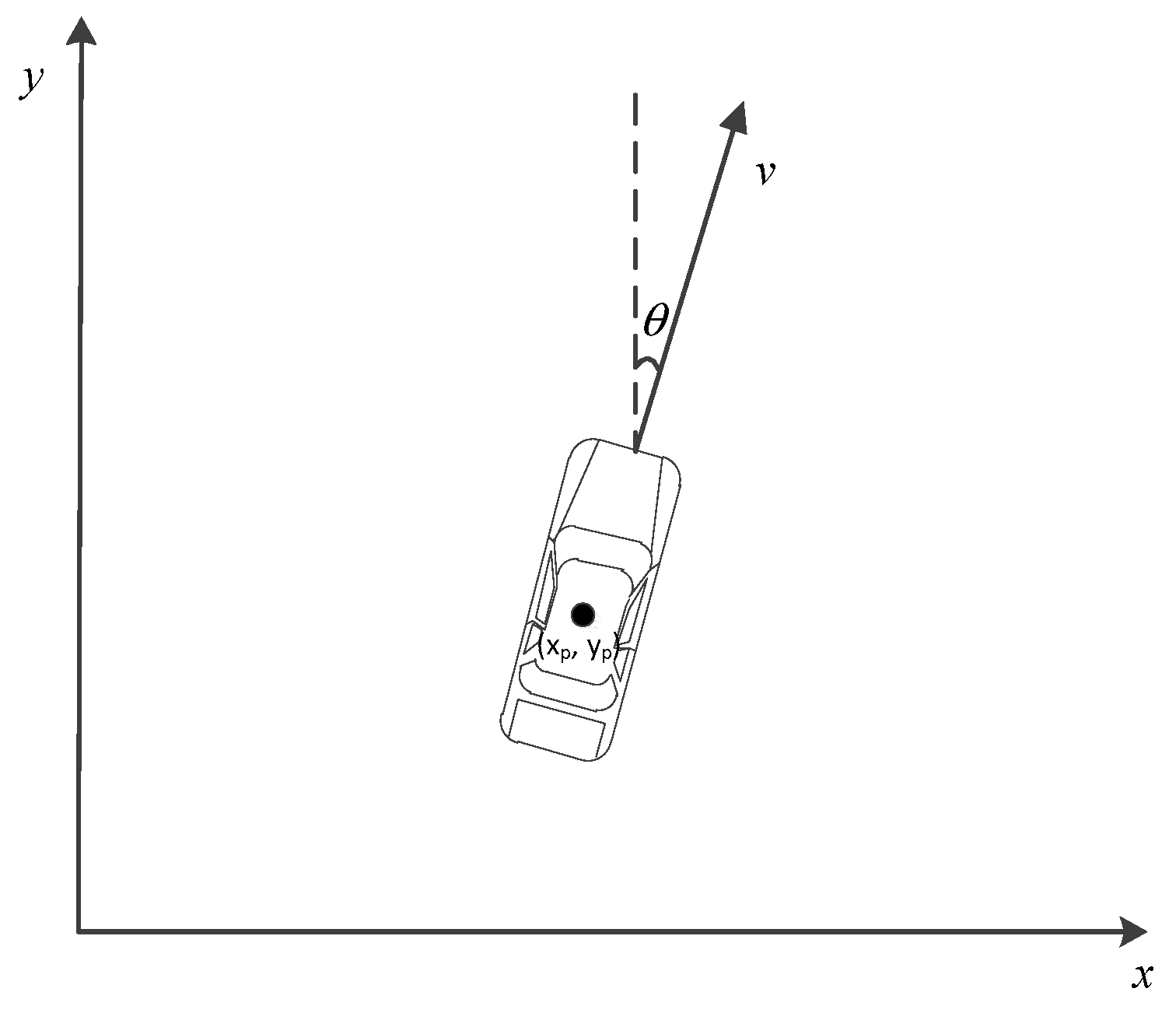
Detected moving vehicles can be extracted from sensor information, and their moving features become accessible. All of the detected vehicles can be modelled with a state vector in the form of Equation (1), as shown in Figure 2.
where is the position, represents the moving direction of the vehicle, and are the velocity and acceleration, respectively, and is the yaw rate of the vehicle. For a vehicle moving along a straight lane, as shown in Figure 3a, the trajectory of the vehicle can be predicted with its moving state, although the trajectory may fail when subject to the conditions in Figure 3b,c. In Figure 3b, the vehicle performs a left lane change, and the vehicle in Figure 3c moves along a winding road. In addition to the moving state, the road structure should be considered when estimating the driving intents of detected vehicles.
By matching the lane marks and road edges with an accurate lane-level map, the accurate position of the vehicle on the map is accessible, as well as the lane number and the road shape. The trajectories of the moving vehicles are strongly influenced by the road shape because drivers tend to follow the center line of a lane, which can be modeled with a quadratic curve, as shown in Equation (2).
where , and are coefficients. In urban environments, the trajectory of a vehicle is decided by the driver and can be divided into the following categories.
- Normal moving (moving along the lane)
- Left change
- Right lane change
- Turn
For most turns at intersections, the driving intent can be estimated by identifying the lane being driven on. For a driver who wants to turn left, he/she will enter the left-turn lane before entering the intersection. Therefore, we mainly discuss normal moving and lane changes in this paper. For a normally moving vehicle, the trajectory is similar to the center line of the lane. On the other hand, a vehicle that is changing its lane is leaving the center line and will enter an adjacent lane. A set of lane change trajectories, obtained from the onboard sensors, are shown in Figure 4. It can be seen that the shapes of the change trajectories are different in both longitudinal and horizontal directions, which increases the difficulty of intent estimation. To estimate the intent of the driver, a state vector of the moving vehicle is constructed.
where are distances between the vehicle and the left lane mark and corresponds to the distance between the vehicle and the right lane mark. is the heading direction of the vehicle, and is the current curvature of its path.
The center line of the lane where the vehicle is moving can also be represented with a state vector:
where is the road direction and is the road curvature. Besides, and are set as half of the lane width. These variables can be obtained with the mentioned quadratic curve mentioned in Equation (1) and road information from the map. The computation of and is attached in Appendix A, and the results are shown in Equations (6) and (7).
Then, the deviation of the vehicle from the lane center can be presented as follows:
where is the chi-square distance between the two vectors, and . is the covariance matrix of the lane state vector, and is the covariance matrix of the vehicle state vector. The moving process is continuous, whereas the maneuvering space is discrete. Intent recognition is performed by mapping a set of continuous features into the discrete maneuvering space. In [13], the value of D is used to estimate the maneuvering intent of the vehicle. If the value is small, the vehicle is assumed to maintain its lane, whereas the vehicle is performing a lane change if the value is larger than a fixed threshold. This method faces a challenge, i.e., a fixed threshold would introduce a high false detection rate. To improve the robustness, a feature vector is constructed as follows:
where is the number of samples that we use in the intent-estimating process and represents the acceleration in the direction of the lane. This vector contains the relationship between the vehicle and lane, as well as the moving state of the detected vehicle. As for a lane change, the prediction is successful if the intention of changing lane is estimated before any part of the vehicle enters the target lane.
Data in Table 1 are used to illustrate the computation of the feature vector. To eliminate the effect of different dimensions, acceleration is measured with m/s2 and yaw is measured with degree/s; the feature vector is normalized with Z-score standardization, which is introduced in Appendix A. The third row and the forth row show the means and standard deviation of the features. Two examples, extracted from a right lane change and a normal moving event, are shown in the fourth row and the fifth row. The Z-scores of the samples are shown in the last two rows.
To obtain accurate driving intent, a learning method that utilizes Gaussian mixture models (GMM) [14] is applied. GMM consists of a basis Gaussian distribution with a linear method. For a feature vector M of length n, the probability distribution function is as follows:
where K is the number of mixture Gaussian distributions and denotes the mixture weights of the mixture function, which satisfy the condition . The GMM can be represented with a set of components and Equation (11):
The expectation maximization algorithm [15] is used to learn the parameters of the GMM, namely, . In this paper, we use a GMM of three possible mixtures related to the three mentioned maneuvers of interest, i.e., normal moving, left lane change and right lane change.
For each state vector M, the posterior probability with each component of the GMM can be obtained, and the best matched component satisfies the following equation:
where is the subscript of the component.
To obtain an intent predictor, trajectories of 200 drivers were collected, including trajectories on straight roads and winding roads, and used in the training process. The data used are shown in Table 2.
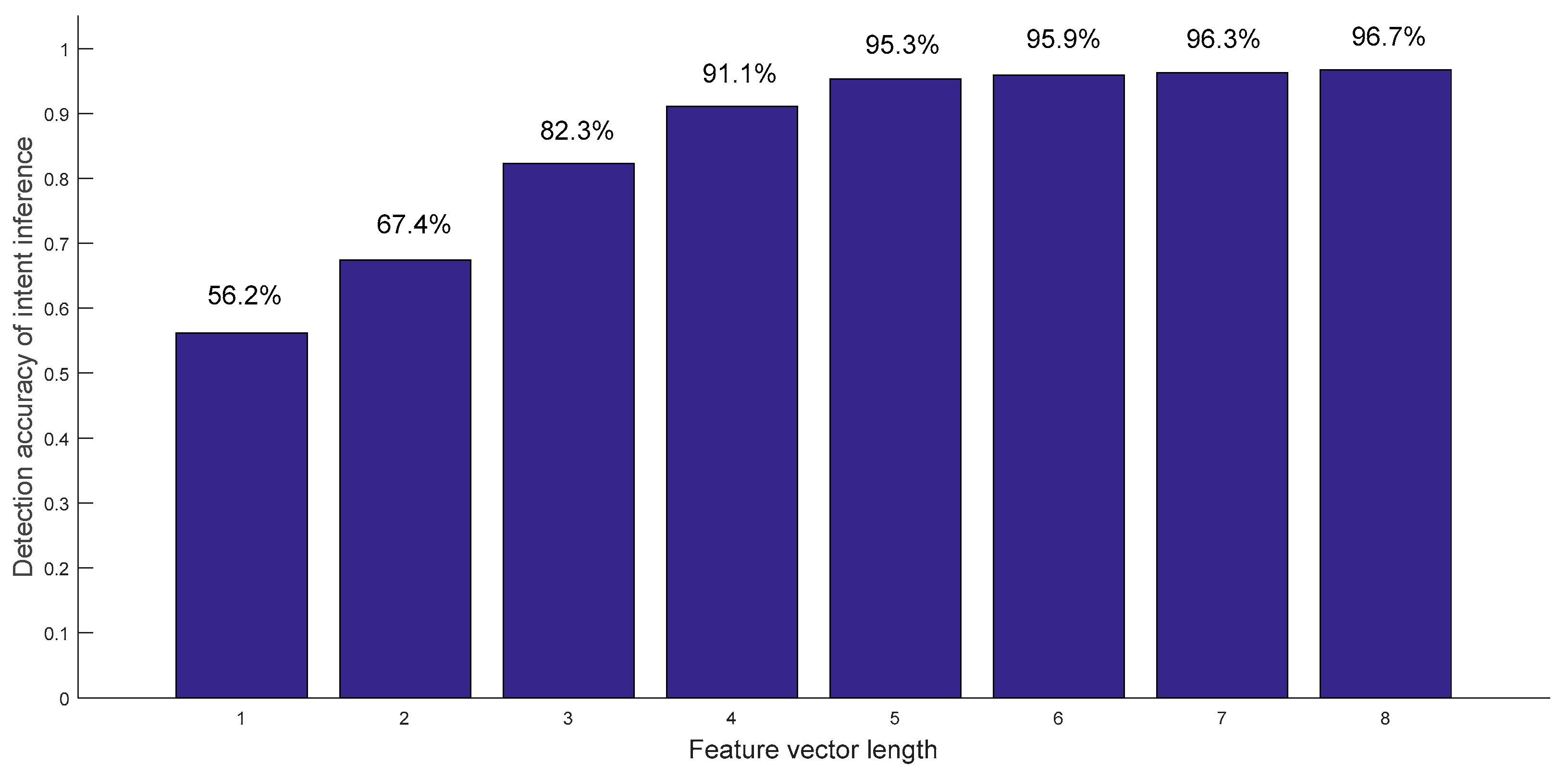
To obtain ideal results, the length of M, i.e., the value of n, should be chosen carefully. The performance is improved with increased n, although the real-time ability of the system decreases, as shown in Figure 5.
The growth rate of the accuracy decreases, and it is limited when n is larger than five. The accuracy reaches 93.5% when n is five. In this paper, the system runs at 25 Hz, and n is set as five. It means that the intent-estimation process needs approximately 200 ms, which is acceptable.
2.3. Trajectory Prediction with Intent and Motion Model
The maneuver intent can be estimated with the GMM-based method, but it is difficult to predict the real trajectory as there are too many realizations for a maneuver. With the initial state, the intended state and the maneuvering information, an ideal trajectory can be obtained. The prediction can be divided into two steps. First, a set of trajectories is generated considering the randomness of driving habits. Then, an appropriate trajectory is selected by considering comfort and duration. The Frenet frame [16] along the lane center line is used to predict the trajectories and then converted to the initial Cartesian coordinates. The lateral component is represented with , and the longitudinal component is . The initial state and final state of the maneuver can be represented with and .
Going a step further, the initial state can be represented with Equation (15):
where is the distance between the initial position of the vehicle and the lane center line. The orientation of the lane center line’s tangent vector is represented by . The normal acceleration of the vehicle is represented as . For the final state of the trajectory, the vehicle is supposed to be moving along the lane center line, and the longitudinal acceleration is a constant value during the maneuvering time. The state can be modeled with the following vector:
If the vehicle is performing a lane change, the value of is the lane width; otherwise, it is set to zero. The duration of a maneuver is limited, and it is set as . A set of trajectories can be obtained by sampling the duration: . The lateral movement of the vehicle can be modeled with a quintic curve [17], as represented in Equation (17):
Combing Equation (16) and (17), the following equation can be obtained:
For the longitudinal movement, a quartic line is used, which can be represented as follows:
The following equation can then be established:
where and a set of trajectories can be obtained by solving the previous two equations with different ending times . To choose the most likely trajectory, two conditions should be considered: the normal acceleration and the duration of the maneuver. The cost function can be summarized into Equation (21):
where is a coefficient that is used to measure the effects of comfort and time, which is selected by analyzing collected data. In this paper, the value of is set as 0.5 to achieve the best result. The selected maneuver trajectory is the trajectory with the smallest cost. All of the generated trajectories are shown in Figure 6. The selected trajectory is marked with the blue dotted line, while the other trajectories are in red.
The long-term trajectory prediction is a desirable result that ignores the current moving state, which is indispensable for trajectory prediction. To increase the accuracy, the long-term predictions and the short-term predictions should be combined. The short-term is achieved by taking advantage of the current moving state of the vehicle and the constant yaw rate and acceleration motion model [18]. The velocity can be obtained as follows:
where and are initial acceleration and velocity of the detected vehicle; and represent the initial yaw rate and moving direction of the detected vehicle. The trajectory can be obtained by integrating the velocity:
where and can be obtained by substituting the initial position into the equation.
We proposed a method that combines the short-term and long-term trajectory predictions by generating a fit. The collected data show that the influence of the ideal trajectory increases with , whereas the influence of the current moving state decreases, and the trajectory can be obtained with Equation (25):
Using this function, the problem becomes a curve-fitting problem, which is related by the parameter t, a proportion of the maneuvering time ranging from zero to one. With our collected data, the influence curve is shown as a red line in Figure 7. decreases much more slowly in the first and third segments than in the second segment, which is in agreement with the practical situation.
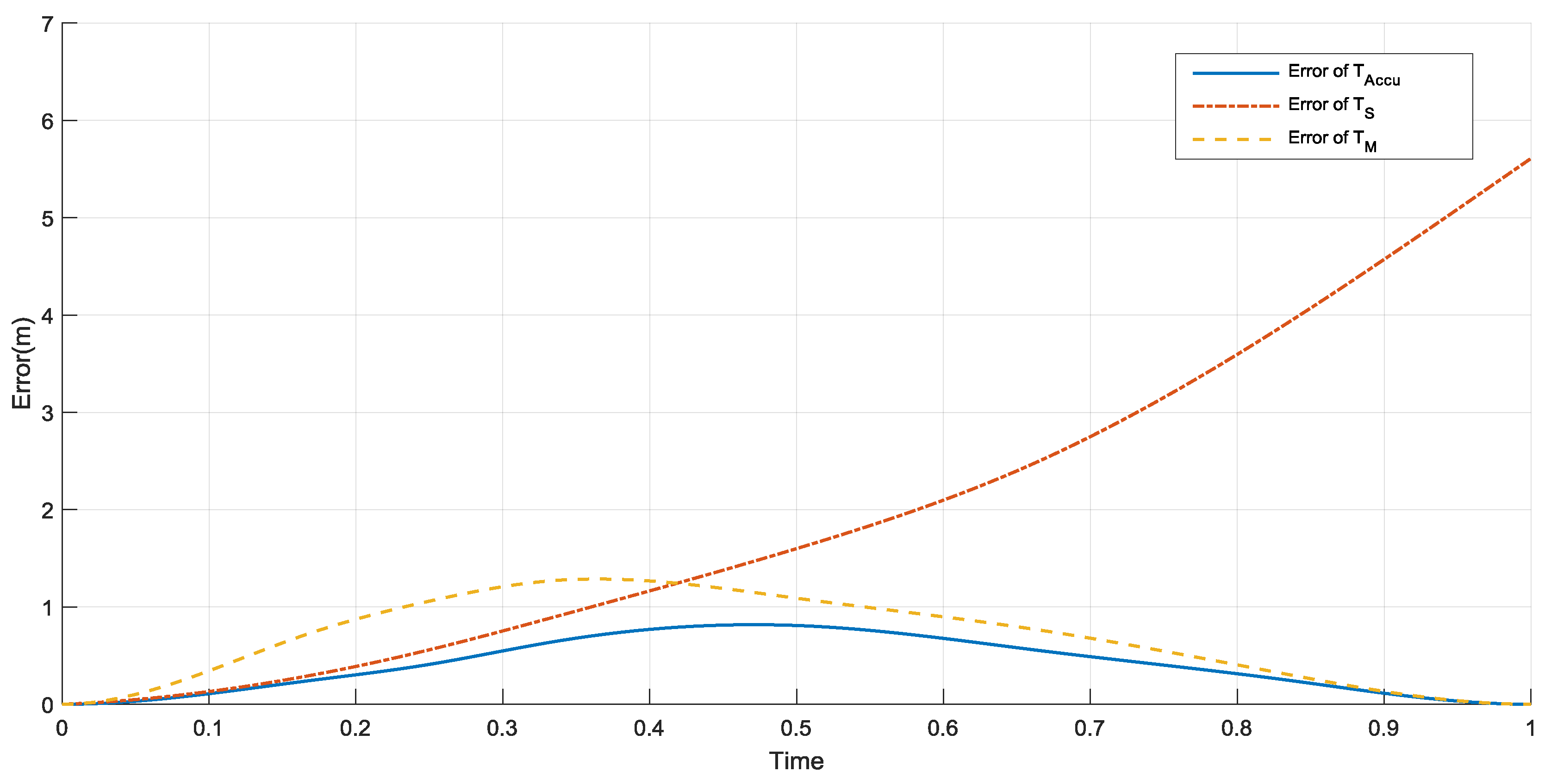
The trajectory prediction error of a typical lane change, which fluctuates with t, is shown in Figure 8. The error in increases from 0 to more than 5 m, which is too large for collision avoidance, and the error in first increases to more than 1 m, but then decreases. On the other hand, the maximum error in is approximately 0.8 m, which is acceptable during the collision detection process. The average errors of , and are 1.98 m, 0.72 m and 0.41 m, which indicate that the accuracy of the fused trajectory is higher.
2.4. Collision Avoidance
The trajectory of the autonomous vehicle is planned using a map of the local environment that contains the road structure, static obstacles and moving obstacles. With the predicted trajectory of detected moving vehicles and the planned trajectory of the autonomous vehicle, collision points will be obtained if they exist. Then, the position of the collision points on the map will be marked. Two methods can be applied by the collision avoidance system: avoiding the collision point in the time dimension and avoiding the collision point in the space dimension. The two methods correspond to acceleration and path re-planning. Appropriate evasive maneuvers will be taken to obtain a longer collision distance and greater driving comfort. As shown in Figure 9a, the detected vehicle is moving at a speed of in the middle lane, and no intent to change lanes is detected. A potential collision point, which is represented by a red point, is obtained using the longitudinal distance and velocity:
where D is the longitudinal distance, and defines the position of the collision point. To guarantee timeliness, a lane change is chosen to avoid a potential collision.
For the scene in Figure 9b, the lane change intent of the detected vehicle can be estimated, and the trajectory is predicted. A collision will occur after T:
To guarantee the safety of the autonomous vehicle, a deceleration is performed to avoid the collision point.
3. Experiments and Discussion
The proposed method was tested on our autonomous vehicle “Intelligent Pioneer” [19,20,21], which is equipped with various sensors, as shown in Figure 10. A Velodyne HDL-64E LIDAR (Velodyne, San Jose, CA, USA), which models the environment by generating a point cloud, is mounted on the top of the vehicle. An IBEO LIDAR (IBEO, Hamburg, Germany) and an SICK LIDAR (SICK, Hamburg, Germany) are mounted in front of the vehicle, and a camera is mounted on the top. A SPAN-CPT and an RTK differential module are used to obtain accurate coordinates of the vehicle and its moving state. The positioning error is less than 5 cm. A computer equipped with a Core i7-3610 CPU is used to process the data.
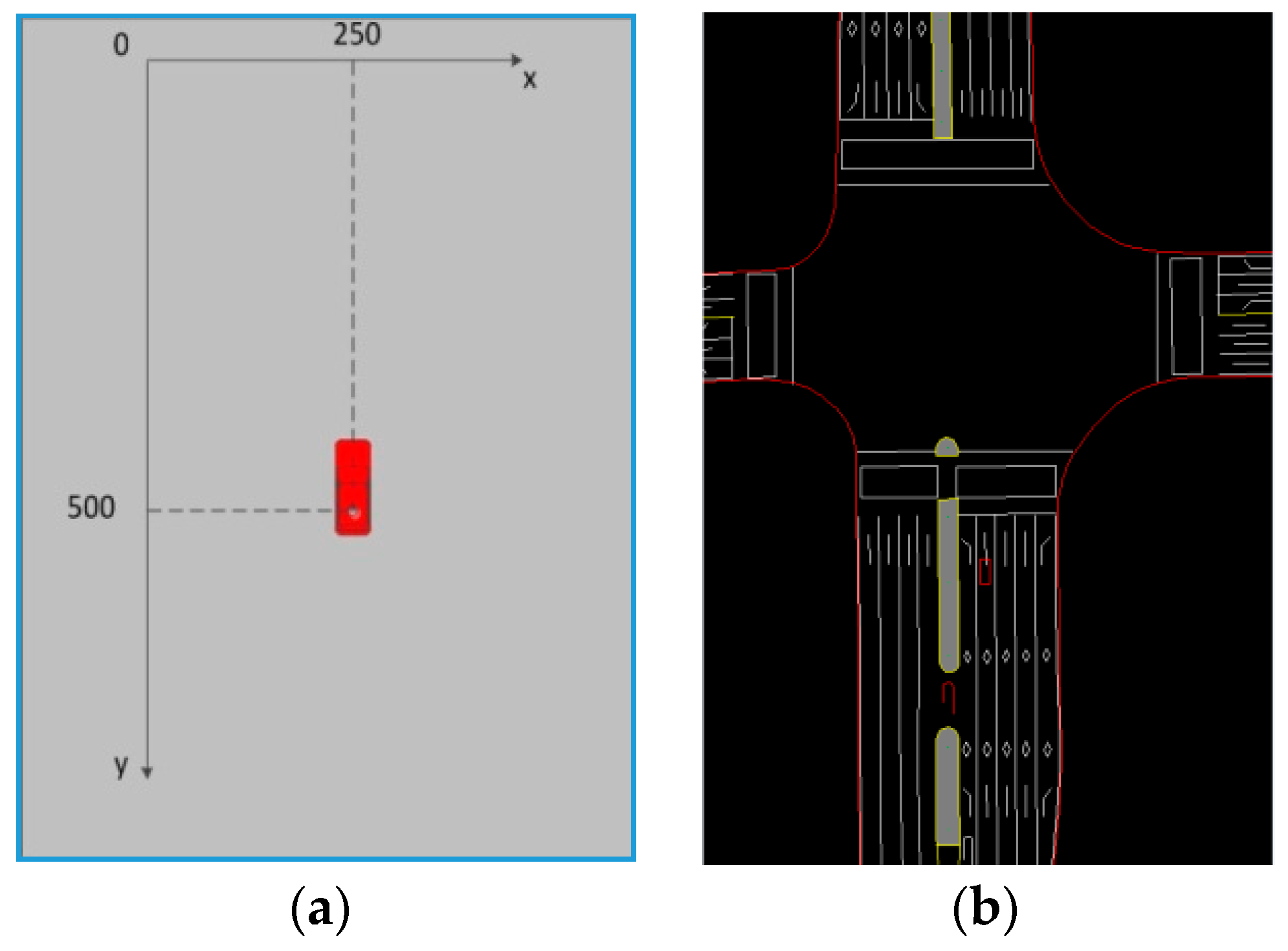
A occupancy grid map with a resolution of 0.2 m is generated to represent the local environment of the intelligent vehicle. The intelligent vehicle is located at (250, 500), and the direction of the vehicle is parallel to the y-axis in the positive direction, as shown in Figure 11a. Grids in the map are set as integer variables ranging from zero to 127 to represent different kinds of obstacles. The value of the grid is set to eight if it is occupied by a static obstacle. Dynamic obstacles are represented by a value of 28, and free areas are denoted with zero. A lane-level accurate map is used to recognize the structure of the environment, including road edges, lane marks and crossings. The localization of the intelligent vehicle on the map can be corrected by matching lane marks on the map with the lane marks detected by the on-board camera. The accurate map is shown in Figure 11b. White lines represent lane marks; sidewalks and stop lines red lines are the edges of the roads; and yellow lines are road barriers that divide the road into two parts. The intelligent vehicle is represented by a red rectangle.
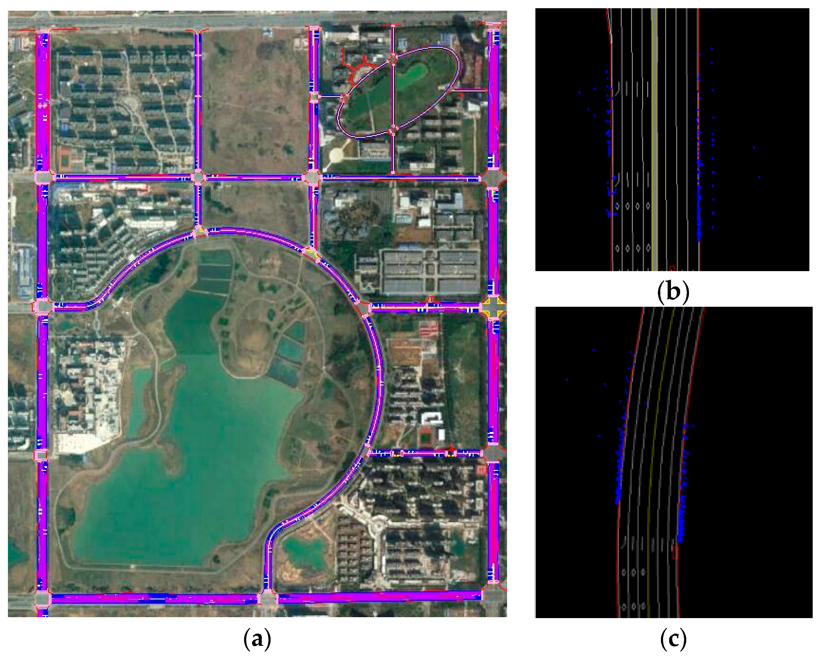
To evaluate the performance of the proposed method, experiments are conducted in an area covering straight roads and winding roads, as shown in Figure 12a. Testing roads are marked in blue and red, including straight roads and winding roads shown in (b) and (c). During the experiments, the vehicle moved autonomously along the roads and performed evasive maneuvers to avoid potential collisions. Vehicles that were moving in the detection area of the autonomous vehicle could be correctly detected. Then, their moving states, mentioned in [1], and the deviation from lane center were recorded and used in the training process. The advantages of the proposed method lie in the accuracy of intent estimation, which increases safety and comfort during collision avoidance.
3.1. Performance of the Intent-Estimation Method
To test the performance of the intent-estimation method, a comparison was conducted between our method and the method applied in [11] that utilized the motion characteristics of detected vehicles and ignores the road structure. For the straight road scenes, 350 events were used in the test, including 278 normal moving events, 38 left lane changes and 34 right lane changes. For the winding road scenes, 233 normal moving events, 38 lane changes and 29 right lane changes were used.
The results of intent estimation on straight roads are shown in Table 3, and the results on winding roads are shown in Table 4. The tables contain precision rate, recall rate and F-score, which were usually used in information retrieval binary classification and pattern recognition. A high precision rate means that an algorithm returns substantially more relevant results than irrelevant ones, and high recall rate means that an algorithm returns most of the relevant results. The F-score is a combination of precision rate and recall rate, which can be used to represent the accuracy of an algorithm. The computation of the precision rate, recall rate and F-score is attached in Appendix B, as well as the confusion matrix of the testing results.
On straight roads, the average F-score of the proposed method is 91.7%, and the average F-score for the method used in [11] is 76.3%. On winding roads, our method achieves an average F-score of 90.5%, and it was 53.2% for the method used in [11]. The accuracy of our method is much higher on both straight roads and winding roads compared with the method used in [11]. The difference between the accuracy of our method on the two kinds of roads is 1.2%, while it is 20.1% for the method used in [11], which indicates that our method is more robust. The experimental results illustrated that our method performs considerably better, especially on winding roads, than the method used in [11].
3.2. Performance of Collision Avoidance Method
Safety is the most important measure for autonomous vehicles and should be ensured during the collision avoidance process. In addition, comfort is another measure that reflects the practicability for passengers. To evaluate the performance of our collision avoidance method, a comparison was conducted between our method and the method used in [8], which ignores the driving intent of other vehicles. Figure 13 shows the distance between the autonomous vehicle and the detected collision point when the collision point is detected on straight roads. It can be seen that collisions will be detected at a longer distance with our method. Under our method, the average distance is 31.6 m, whereas it is 23.2 m under the method used in [8]. The difference of the average collision detection distance for the two methods is 8.4 m.
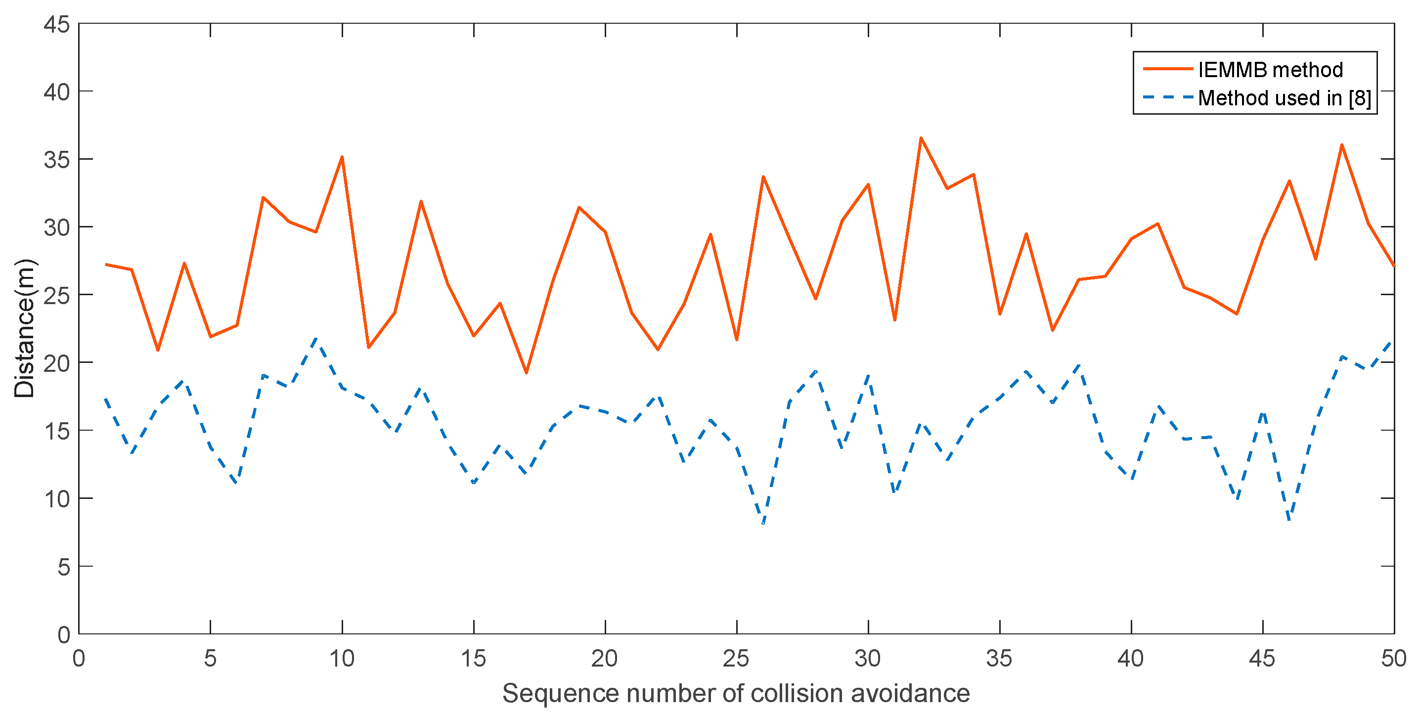
Figure 14 shows the collision detection distance on winding roads. Compared with the distance on straight roads, it is shorter on winding roads, and the general tendency is similar. The average distance of our method is 27.4 m, and the shortest distance is 19.2 m; in contrast, these values are 15.6 m and 8.1 m under the method used in [8]. The difference of average collision detection distance for the two methods is 11.8 m. Potential collisions can be detected at longer distances with our method, because the trajectories of the detected vehicles can be predicted by combining the estimated intent and motion model. Then, evasive actions can be performed to avoid collisions with a sufficient distance.
In addition to safety, comfort is another factor that must be considered when evaluating the collision avoidance method. It can be inferred from [22] that the yaw rate and acceleration play import roles in driving comfort. With increasing yaw rate and acceleration, comfort decreases. Figure 15 shows the peaks of the yaw rate during collision avoidance maneuvers when applying the IEMMB collision avoidance method and the method used in [8]. It can be seen that the yaw rate of the IEMMB method is mainly concentrated in the range of −10 to 10, whereas a considerable portion of the yaw rate of the other method exceeds the range of −10 to 10. A smaller yaw rate indicates that our method improves the comfort of autonomous driving.
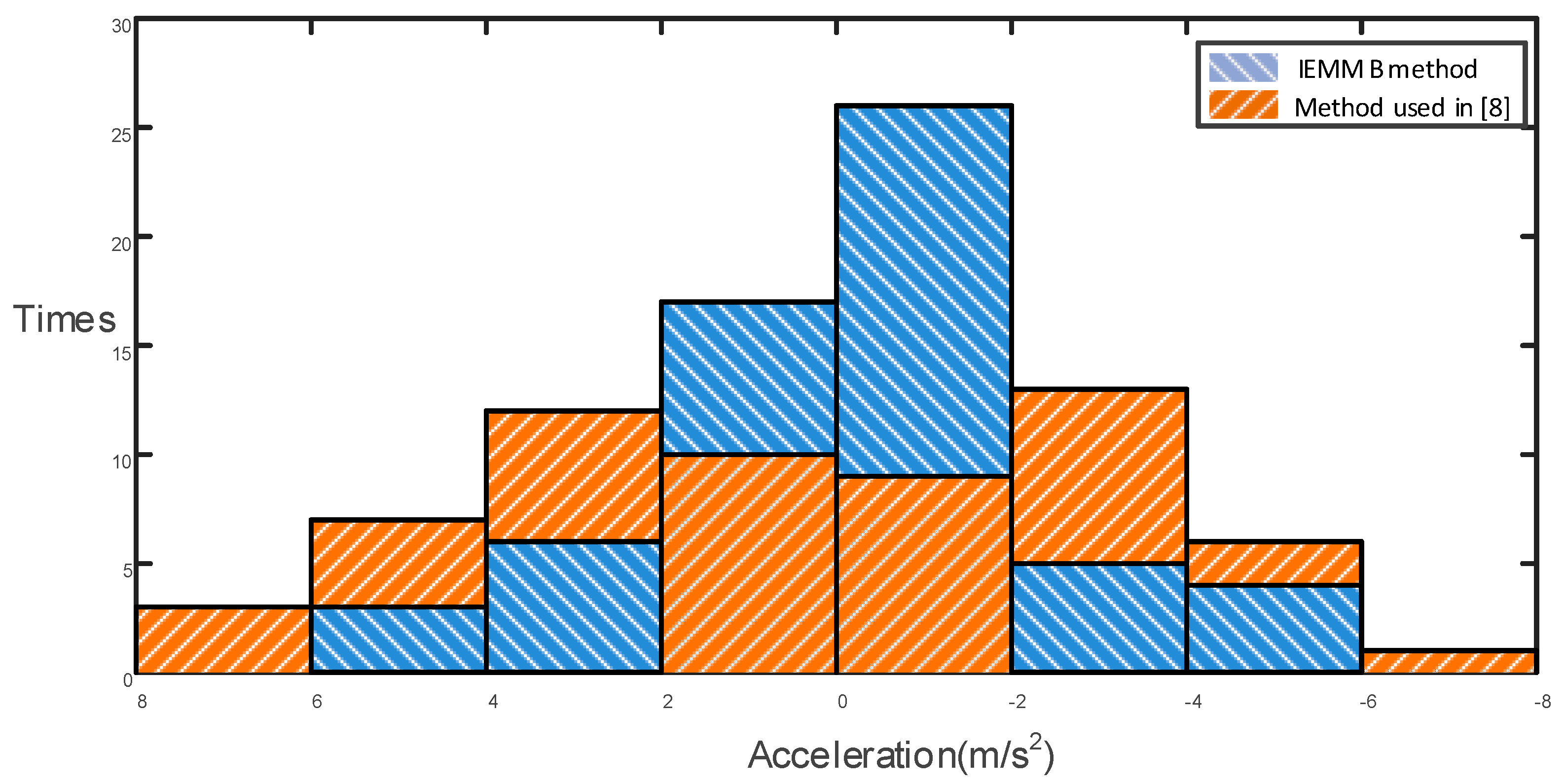
Figure 16 shows the maximum accelerations during collision avoidance under our method and under the method presented in [8]. It can be seen that the maximum acceleration of our method is mainly distributed in the range of −2 to 2 m/s2, whereas the maximum acceleration of the method used in [8] often exceeds this range. This indicates that the evasive actions in [8] are fiercer and that our method results in more comfortable collision avoidance actions.
3.3. Typical Collision Avoidance Scenes
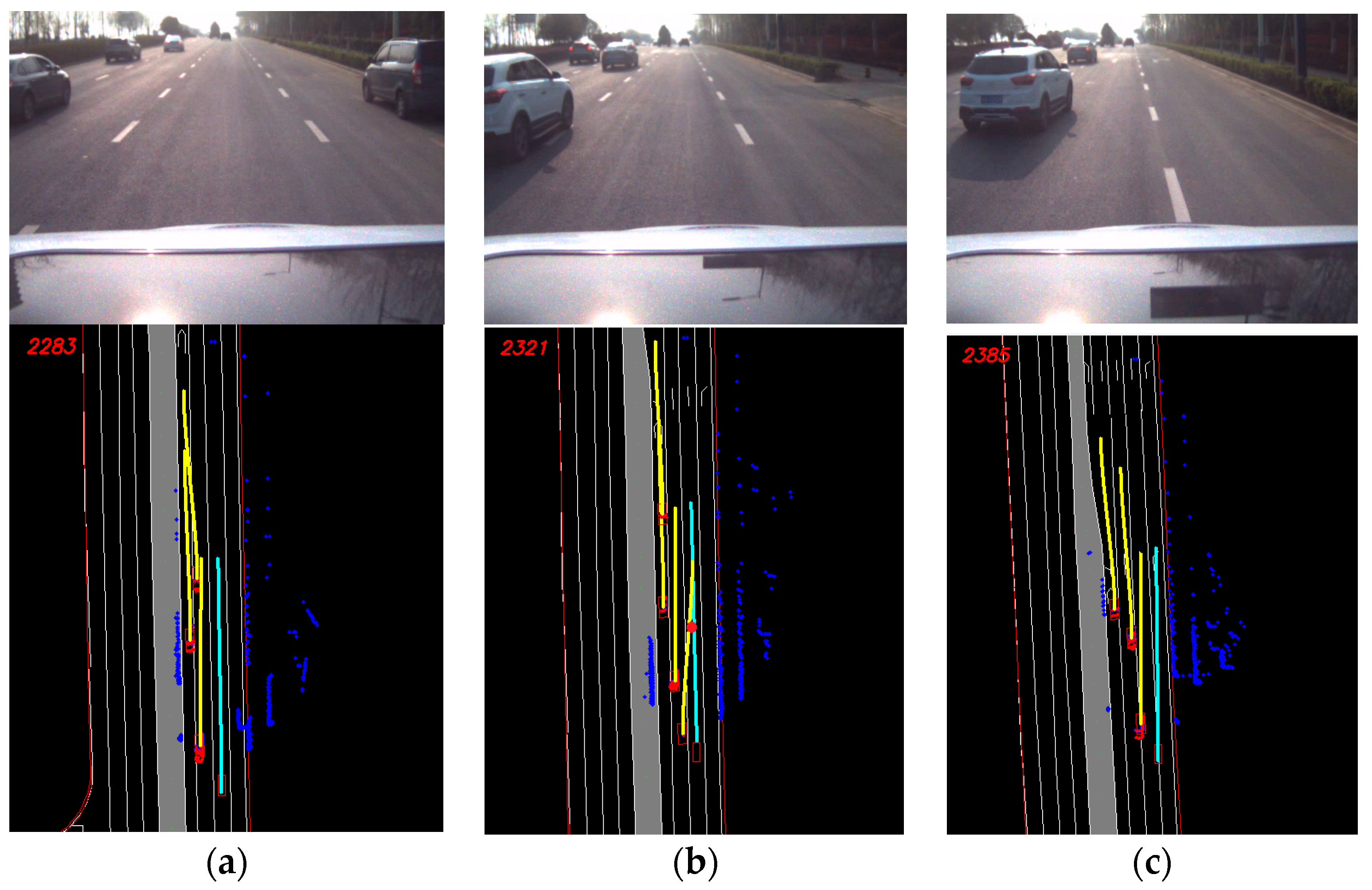
A typical collision avoidance scene on a straight road is shown in Figure 17. The first row shows the real scene, and the second row shows the path planning result of the autonomous vehicle during the collision avoidance. As shown in Figure 17a, the autonomous vehicle is keeping its lane, and three vehicles are detected. The left top vehicle is performing a left lane change, and two vehicles are moving along their lanes. In Figure 17b, a new vehicle is detected, which is taking a right lane change. The trajectory of the white car is predicted with the intent-estimation- and motion-model-based method, and a potential collision between the vehicle and the autonomous vehicle is detected, which is marked with a red circle. Then, a deceleration is executed, and a right lane change path is generated to avoid the collision.
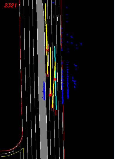
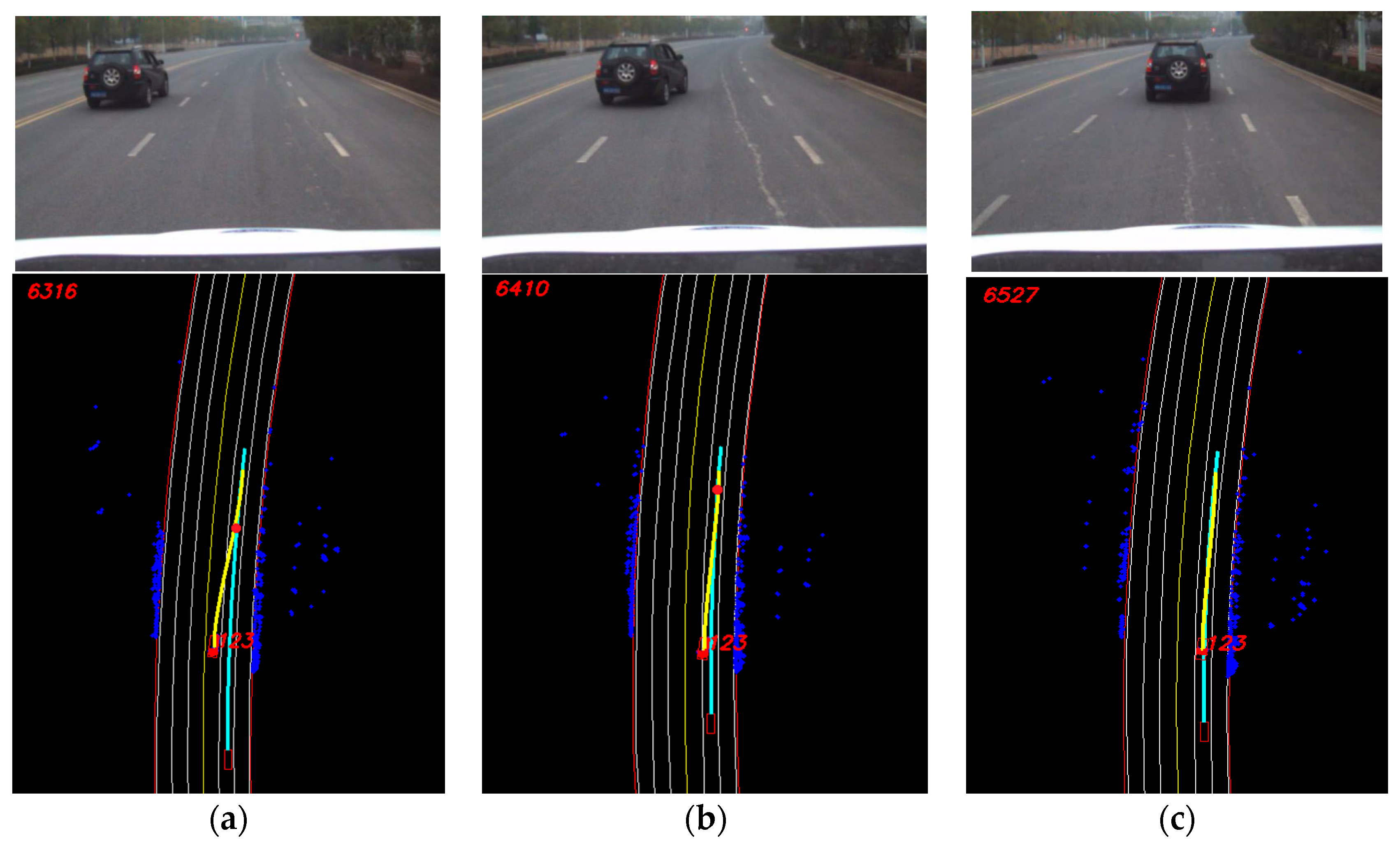
Figure 18 shows typical collision avoidance scenes when the autonomous vehicle is moving on a winding road. The detected vehicle is marked with a red rectangle, and its sequence number is 123. In the first picture, the driving intent of the vehicle, i.e., a right lane change, is inferred, and a collision point is obtained. Then, a deceleration is performed by the autonomous vehicle to avoid a potential collision. The distance between the autonomous vehicle and the front vehicle decreased first from 23 m to 16 m and then remained greater than 16 m in the following scenes. The maximum acceleration is 2.5 m/s2.
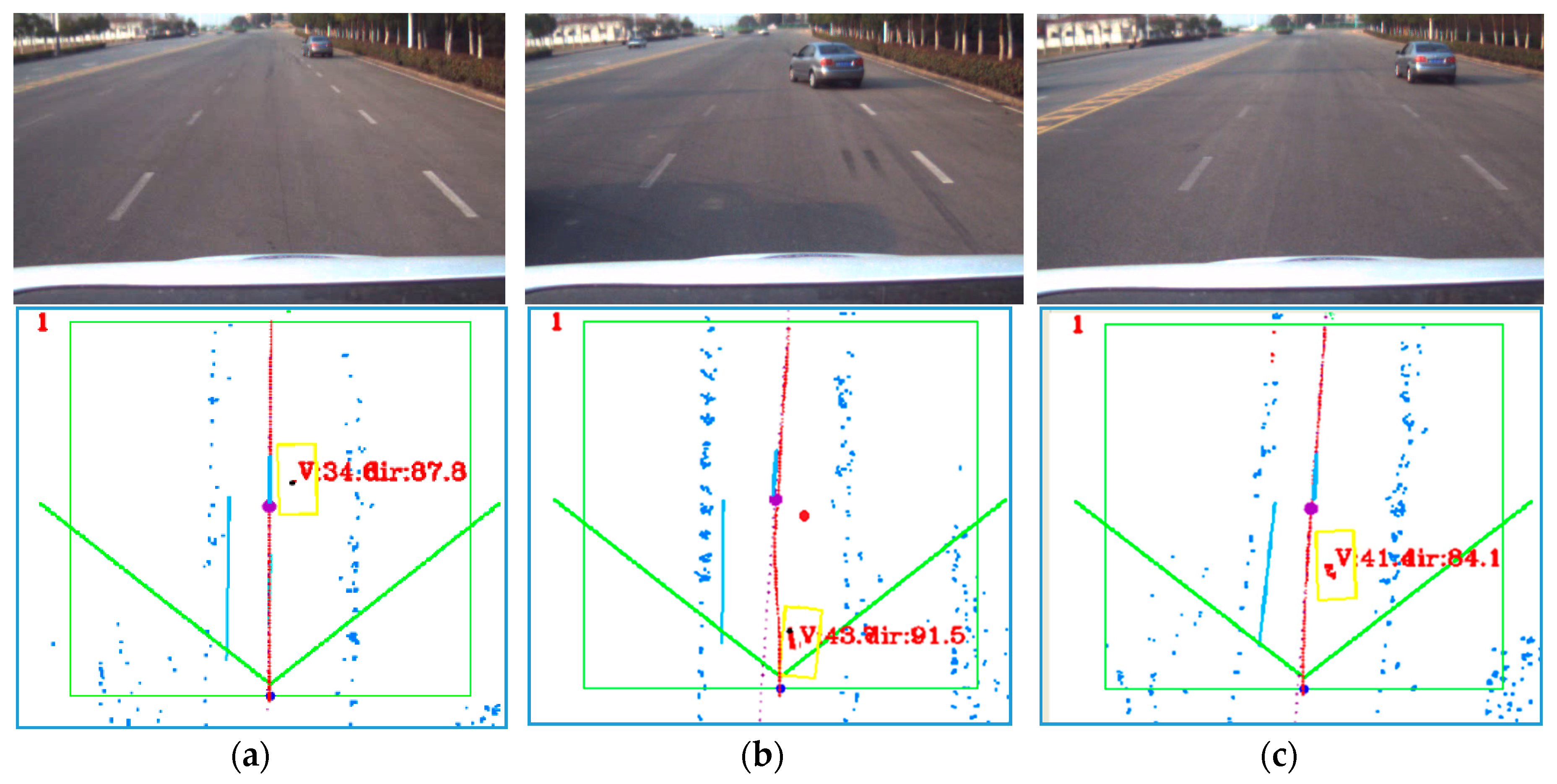
Figure 19 shows a typical collision avoidance process when applying the collision method used in [8], which ignores the driving intent of the detected vehicle. The detected vehicle is marked with red points, which are circled by a yellow rectangle. The velocity and moving direction of the detected vehicle, as well as the planned path of the autonomous vehicle are marked in red. The green box represents the dynamic obstacle detection range of the three-dimensional LIDAR, and the area between the two green lines illustrates the detection area of the IBEO LIDAR. A collision point was not detected until the detected vehicle entered the target lane as shown in Figure 18b. A lane change is simultaneously performed by the autonomous vehicle to avoid the potential collision. The collision point was detected too late, which resulted in a distance of 7.9 m between the autonomous vehicle and the detected vehicle.
4. Conclusions
To decrease the false detection rate of collisions with vehicles on winding roads and the missed detection rate of collisions with maneuvering vehicles, this article introduced an intent-estimation- and motion-model-based collision avoidance method for autonomous vehicles in urban environments. The maneuvering intent of detected vehicles is estimated by combining the vehicles’ moving state and the road structure. A GMM is used to train the intent predictor and then used to predict the intent of detected vehicles. With the driving intent, an ideal long-term trajectory can be obtained by making a balance between timeliness and comfort. The short-term trajectory can be obtained by utilizing a constant yaw rate and acceleration motion model. Then, the long-term trajectory and the short-term trajectory are combined by generating a linear fit to predict an accurate trajectory. Finally, potential collisions are detected and can be avoided in the space dimension or in the time dimension by taking evasive actions in advance. The experimental results demonstrated that the GMM-based intent estimation method achieves a high accuracy, 91.7% on a straight road and 90.5% on a winding roads, and the intent-estimation- and motion-model-based collision avoidance method improves the safety and comfort of the intelligent vehicle on both straight roads and winding roads. The detection distance of potential collisions, which is crucial in collision avoidance, is increased by more than 8 m. The yaw rate and acceleration during collision avoidance are decreased compared with the traditional method. Our future work will focus on expanding the scope of application of intent estimation, for instance including the moving intent of pedestrians and bicycles. Besides, a further research on the road model will be conducted to increase the accuracy of intent estimation.
Acknowledgments
We would like to acknowledge all of our team members, whose contributions were essential for this paper. We would also like to acknowledge the support of National Nature Science Foundations of China (Grant Nos. 61503362, 61305111, 61304100, 91420104),National Nature Science Foundations of Anhui Province (Grant No. 1508085MF133) and the Guangdong Province Science and Technology Plan (Grant No. 2016B090910002).
Author Contributions
All six authors contributed to this work. Rulin Huang was responsible for the literature search, algorithm design and data analysis. Huawei Liang, Pan Zhao and Biao Yu made substantial contributions to the planning and design of the experiments. Rulin Huang was responsible for the writing of the paper, and Xinli Geng helped modify the paper. Finally, all listed authors approved the final manuscript.
Conflicts of Interest
The authors declare no conflict of interest.
Appendix A
Computation of road direction and road curvature :
where is the quadratic curve used to model the lane.
Z-score standardization:
The standard score of a raw score is:
where is the mean of the population and is the standard deviation of the population.
Appendix B
1. Computation of precision rate, recall rate and F-score:
2. Confusion matrix on straight roads
| Our Method | Predicted Results | Normal moving | Left lane change | Right lane change | |
| Ground Truth | |||||
| Normal Moving | 270 | 4 | 4 | ||
| Left lane change | 4 | 34 | 0 | ||
| Right lane change | 4 | 0 | 30 | ||
| Method in [11] | Predicted Results | Normal moving | Left lane change | Right lane change | |
| Ground Truth | |||||
| Normal Moving | 249 | 16 | 13 | ||
| Left lane change | 10 | 28 | 0 | ||
| Right lane change | 9 | 0 | 25 | ||
3. Confusion matrix on winding roads
| Our Method | Predicted Results | Normal moving | Left lane change | Right lane change | |
| Ground Truth | |||||
| Normal Moving | 221 | 7 | 5 | ||
| Left lane change | 5 | 33 | 0 | ||
| Right lane change | 4 | 0 | 25 | ||
| Method in [11] | Predicted Results | Normal moving | Left lane change | Right lane change | |
| Ground Truth | |||||
| Normal Moving | 176 | 33 | 24 | ||
| Left lane change | 21 | 17 | 0 | ||
| Right lane change | 15 | 0 | 14 | ||
References
- Pawan, D. Road Safety and Accident Prevention in India: A review. IJAET 2014, 5, 64–68. [Google Scholar]
- IEEE SPECTRUM. Available online: http://spectrum.ieee.org/transportation/advanced-cars/autonomous-vehicles-complete-darpa-urban-challenge (accessed on 1 November 2007).
- The New York Times. Available online: https://www.nytimes.com/interactive/2016/07/01/business/inside-tesla-accident.html?_r=0,July (accessed on 12 July 2016).
- State of California Department of Motor Vehicles. Available online: https://www.dmv.ca.gov/portal/wcm/connect/3946fbb8-e04e-4d52-8f80-b33948df34b2/Google_021416.pdf?MOD=AJPERES (accessed on 23 February 2016).
- Urmson, C.; Anhalt, J.; Bagnell, D.; Baker, C.; Bittner, R.; Clark, M.N.; Dolan, J.; Duggins, D.; Galatali, T.; et al. Autonomous Driving in Urban Environments: Boss and the Urban Challenge. J. Field Robot. 2008, 25, 425–466. [Google Scholar] [CrossRef]
- Ferguson, D. Prediction, Tracking and Avoidance of Dynamic Obstacle in Urban Environments. In Proceedings of the IEEE Intelligent Vehicles Symposium, Eindhoven, The Netherlands, 4–6 June 2008. [Google Scholar]
- Montemerlo, M. Junior: The Stanford Entry in the Urban Challenge. J. Field Robot. 2008, 25, 569–597. [Google Scholar] [CrossRef]
- Xin, Y.; Liang, H.; Mei, T.; Huang, R.; Chen, J.; Zhao, P.; Sun, C.; Wu, Y. A New Dynamic obstacle Collision Avoidance System for Autonomous Vehicles. Int. J. Robot. Autom. 2015, 30, 113–131. [Google Scholar] [CrossRef]
- Stéphanie, L. Context-based Estimation of Driver Intent at Road Intersections. In Proceedings of the IEEE Symposium on Computational Intelligence in Vehicles and Transportation Systems, Singapore, 16–19 April 2013. [Google Scholar]
- Liebner, M. Velocity-Based Driver Intent Inference at Urban Intersections in the Presence of Preceding Vehicles. Intell. Trans. Syst. Mag. 2013, 5, 10–21. [Google Scholar] [CrossRef]
- Gadepally, V.N. Estimation of Driver Behavior for Autonomous Vehicle Applications. Ph.D. Theses, The Ohio State University, Columbus, OH, USA, 2013. [Google Scholar]
- Huang, R.; Liang, H.; Chen, J.; Zhao, P.; Du, M. An intent inference based dynamic obstacle avoidance method for intelligent vehicle in structured environment. In Proceedings of the IEEE International Conference on Robotics and Biomimetics, Zhuhai, China, 6–9 December 2015. [Google Scholar]
- Houenou, A.; Bonnifait, P.; Cherfaoui, V.; Yao, W. Vehicle trajectory prediction based on motion model and maneuver recognition. In Proceedings of the IEEE Intelligent Vehicles Symposium, Gold Coast, Australia, 23–26 June 2013. [Google Scholar]
- Yu, D.; Deng, L. Gaussian Mixture Models. In Automatic Speech Recognition; Springer: London, UK, 2015; pp. 13–21. [Google Scholar]
- Shu, K.N.; Krishnan, T.; Mclachlan, G.J. The EM Algorithm. In Handbook of Computational Statistics; Springer: Berlin/Heidelberg, Germany, 2012; pp. 139–172. [Google Scholar]
- Werling, M.; Ziegler, J.; Kammel, S.; Thrun, S. Optimal trajectory generation for dynamic street scenarios in a Frenét Frame. In Proceedings of the IEEE International Conference on Robotics and Automation, Anchorage, AK, USA, 3–8 May 2010. [Google Scholar]
- Takahashi, A.; Hongo, T.; Ninomiya, Y.; Sugimoto, G. Local Path Planning and Motion Control for AGV in Positioning. In Proceedings of the IEEE/RSJ International Workshop on Intelligent Robots and Systems, Tsukuba, Japan, 4–6 September 1989; pp. 392–397. [Google Scholar]
- Schubert, R.; Richter, E.; Wanielik, G. Comparison and evaluation of advanced motion models for vehicle tracking. In Proceedings of the International Conference on Information Fusion, Cologne, Germany, 30 June–3 July 2008. [Google Scholar]
- Liu, J.; Liang, H.; Wang, Z.; Chen, X. A Framework for Applying Point Clouds Grabbed by Multi-Beam LIDAR in Perceiving the Driving Environment. Sensors 2015, 15, 21931–21956. [Google Scholar] [CrossRef] [PubMed]
- Du, M.; Mei, T.; Liang, H.; Chen, J.; Huang, R.; Zhao, P. Drivers’ Visual Behavior-Guided RRT Motion Planner for Autonomous On-Road Driving. Sensors 2016, 16, 102. [Google Scholar] [CrossRef] [PubMed]
- Chen, J.; Zhao, P.; Liang, H.; Mei, T. Motion Planning for Autonomous Vehicle Based on Radial Basis Function Neural Network in Unstructured Environment. Sensors 2014, 14, 17548–17566. [Google Scholar] [CrossRef] [PubMed]
- Karjanto, J.; Yusof, N.M. Comfort Determination in Autonomous Driving Style. In Proceedings of the AutoUI, Nottingham, UK, 1–3 September 2015. [Google Scholar]
Figure 1.
Structure of the collision avoidance method. Driving intent estimation and trajectory prediction are the two main components of this method.
Figure 1.
Structure of the collision avoidance method. Driving intent estimation and trajectory prediction are the two main components of this method.
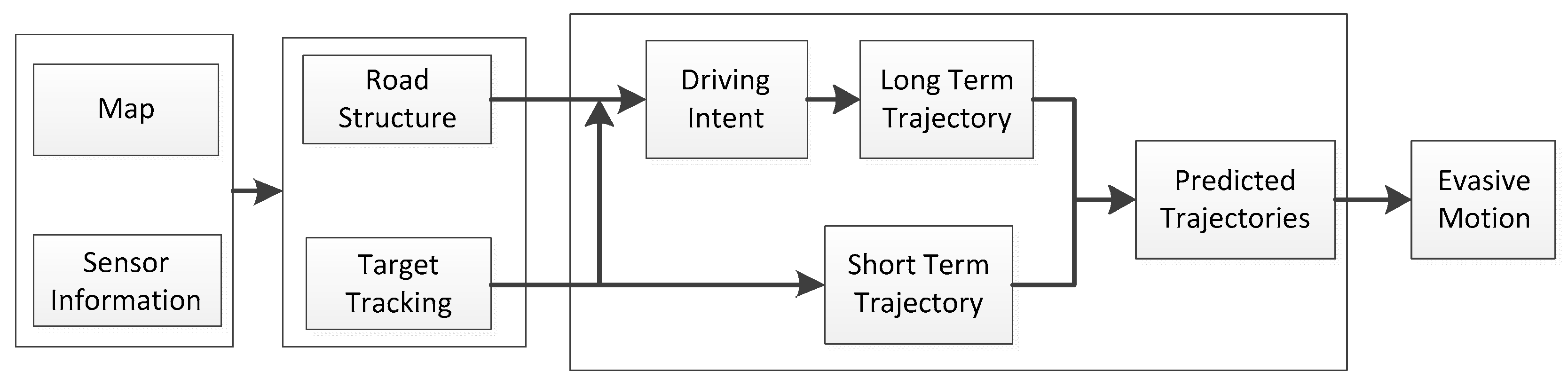
Figure 2.
Moving state of a vehicle.

Figure 3.
Typical trajectory: (a) normal moving; (b) lane change; (c) normal moving on a winding road.
Figure 3.
Typical trajectory: (a) normal moving; (b) lane change; (c) normal moving on a winding road.
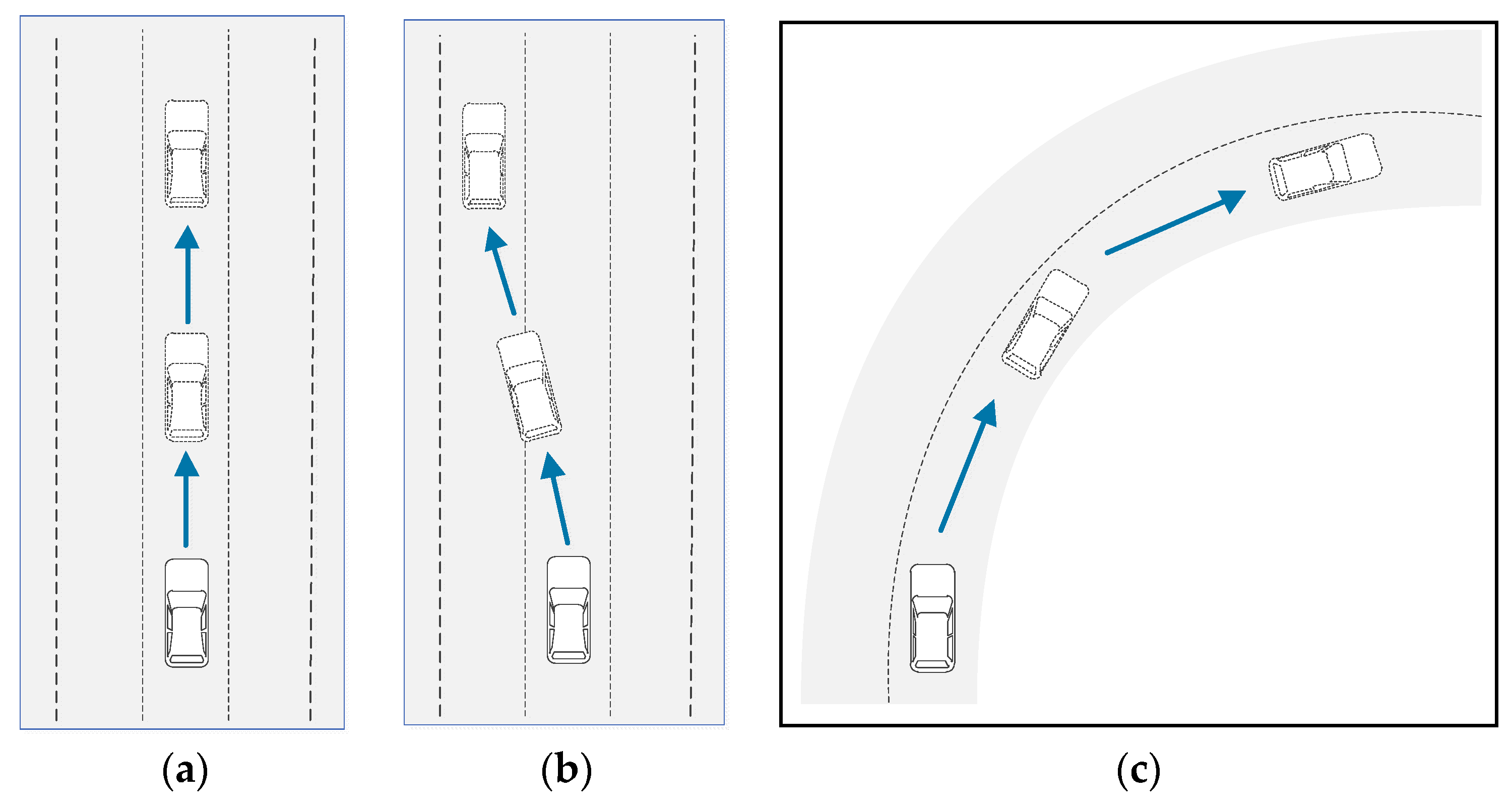
Figure 4.
Lane changes.
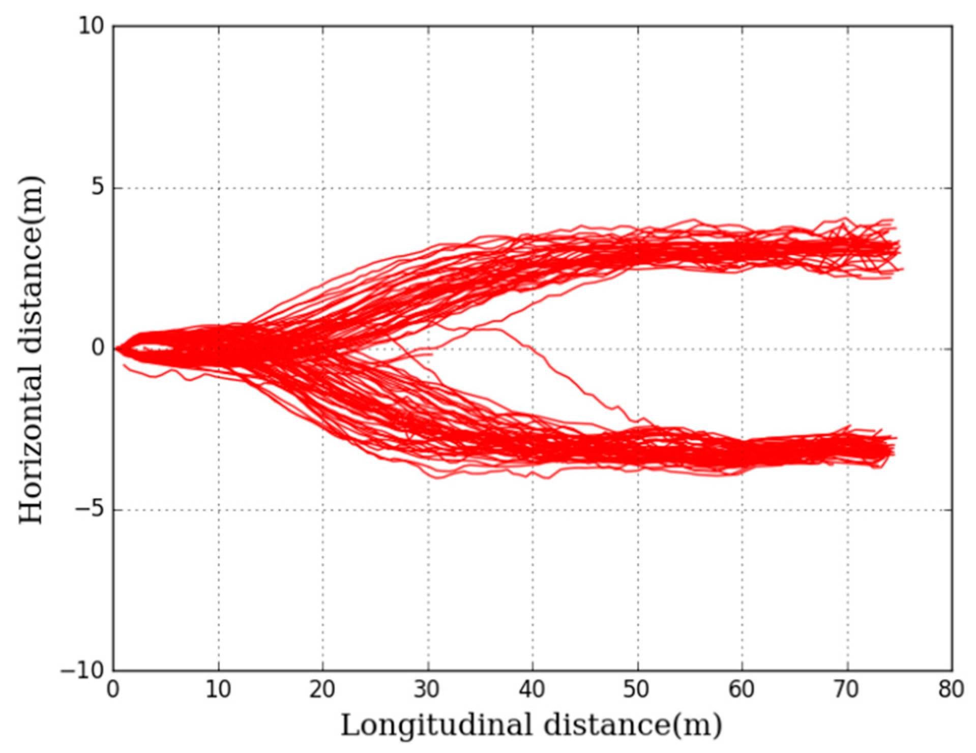
Figure 5.
Relationship between the length of feature vector M and the accuracy of intent estimation. The accuracy grows with the length while the growth rate is decreasing.
Figure 5.
Relationship between the length of feature vector M and the accuracy of intent estimation. The accuracy grows with the length while the growth rate is decreasing.

Figure 6.
Trajectory candidates, which are represented with red lines, and the selected ideal trajectory, which is represented with a blue line. The selection of the ideal trajectory makes a balance of timeliness and driving comfort.
Figure 6.
Trajectory candidates, which are represented with red lines, and the selected ideal trajectory, which is represented with a blue line. The selection of the ideal trajectory makes a balance of timeliness and driving comfort.
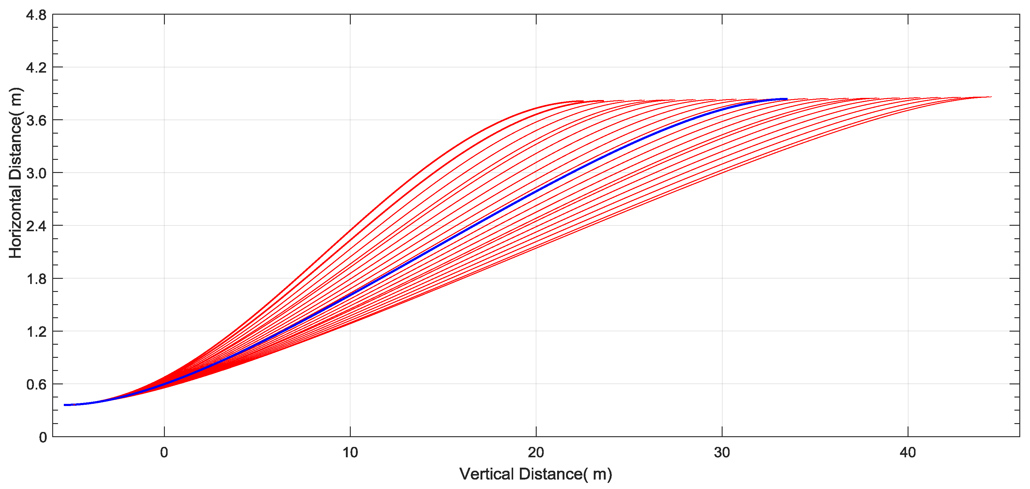
Figure 7.
Influence curve. The influence of the ideal trajectory decreases slightly in the first stage and third stage while it falls fast in the second stage.
Figure 7.
Influence curve. The influence of the ideal trajectory decreases slightly in the first stage and third stage while it falls fast in the second stage.
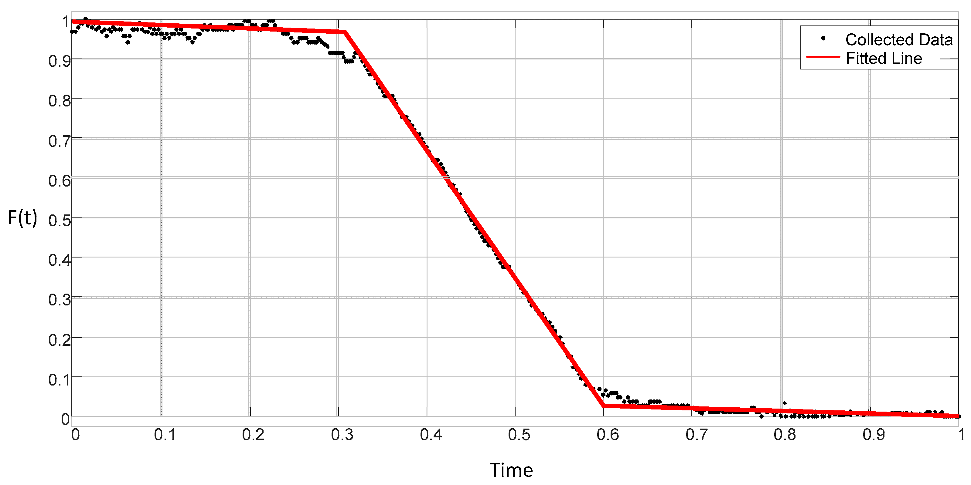
Figure 8.
Trajectory error comparison. The error of increases throughout the maneuver; while the errors of and increase firstly and then decrease. is more in line with the real trajectory.
Figure 8.
Trajectory error comparison. The error of increases throughout the maneuver; while the errors of and increase firstly and then decrease. is more in line with the real trajectory.

Figure 9.
Collision avoidance: (a) collision avoidance in the space dimension; (b) collision avoidance in the time dimension.
Figure 9.
Collision avoidance: (a) collision avoidance in the space dimension; (b) collision avoidance in the time dimension.
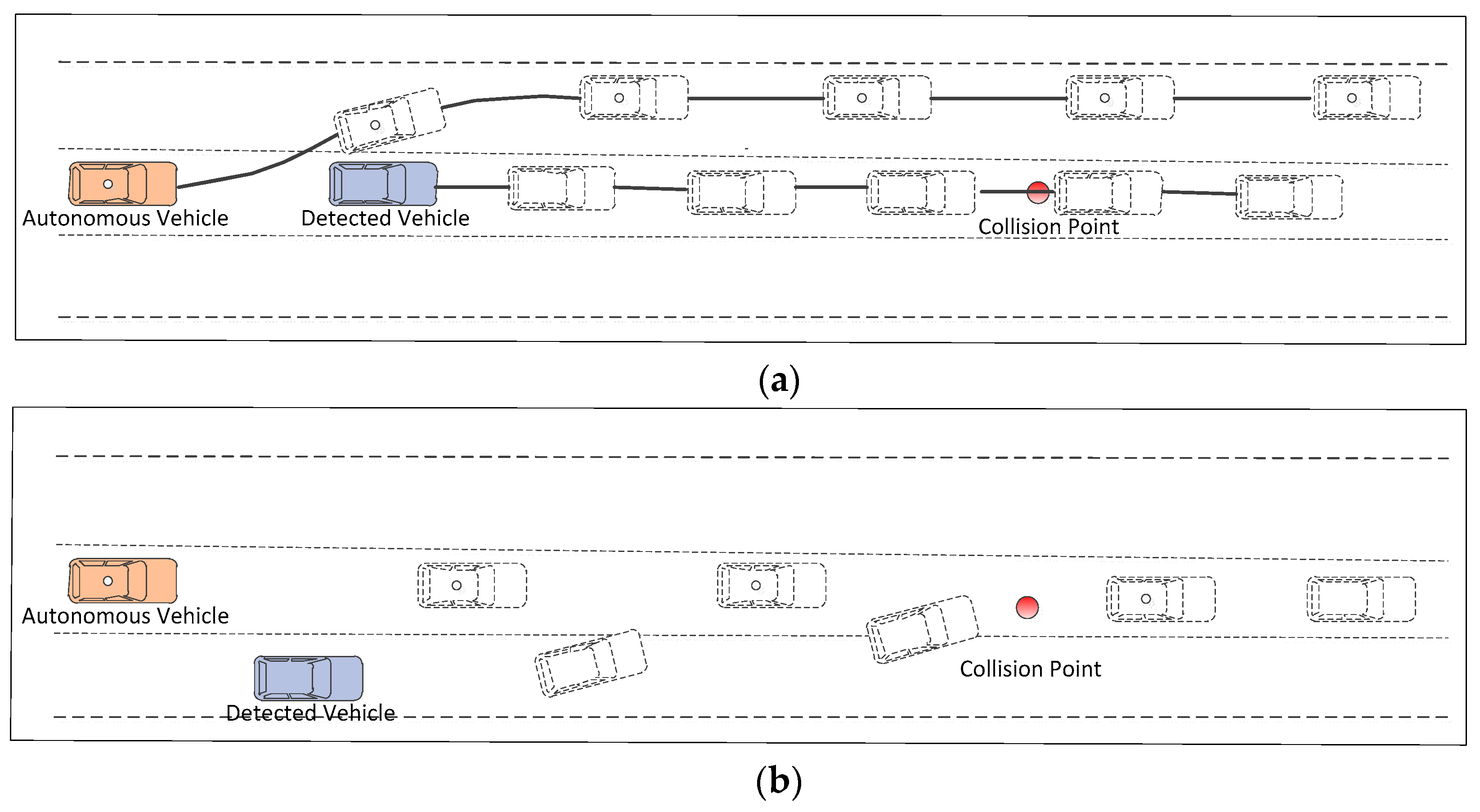
Figure 10.
Intelligent Pioneer. The testing platform is equipped with a variety of sensors including a three-dimensional LIDAR, a two-dimensional LIDAR and a camera.
Figure 10.
Intelligent Pioneer. The testing platform is equipped with a variety of sensors including a three-dimensional LIDAR, a two-dimensional LIDAR and a camera.
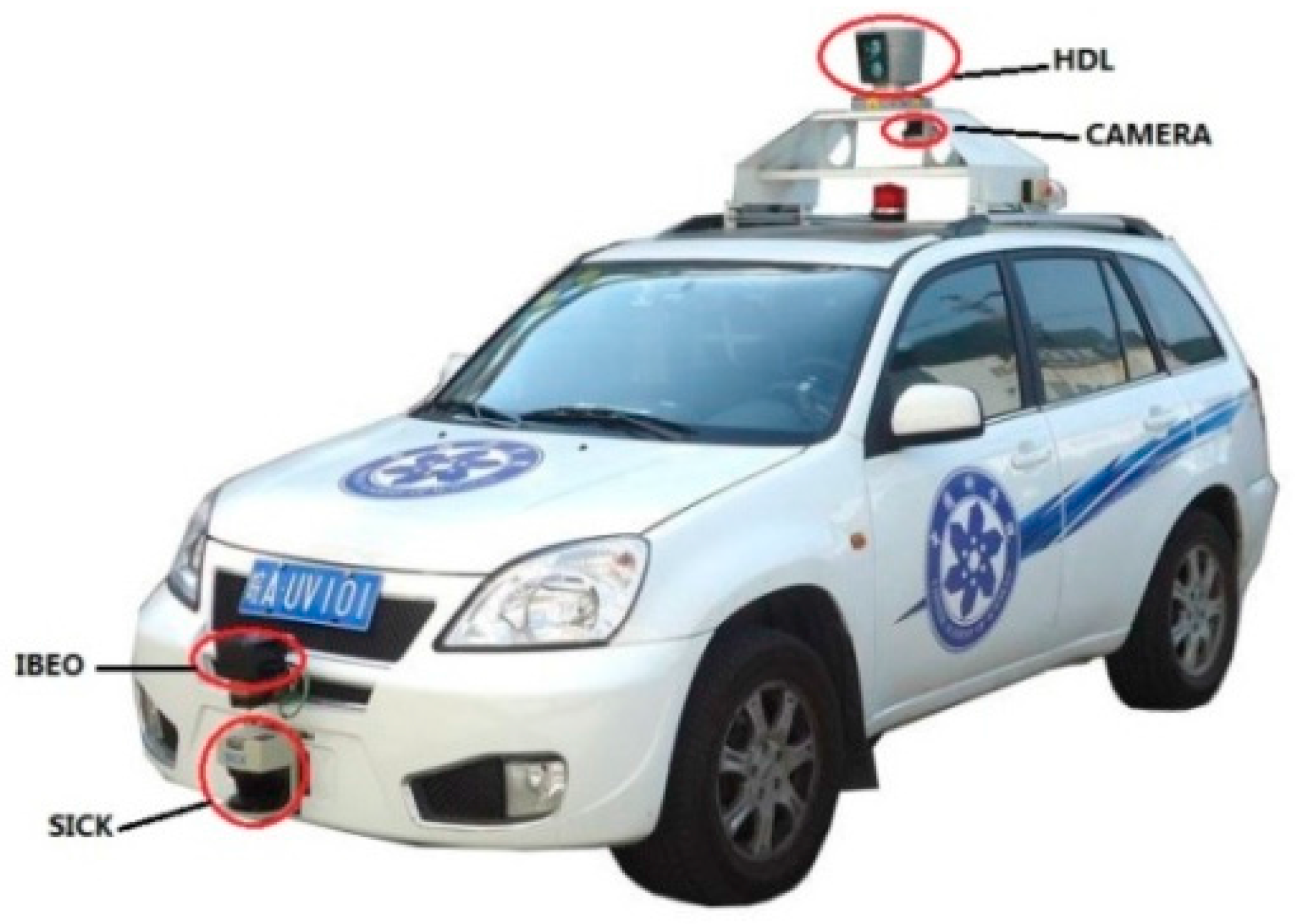
Figure 11.
System introduction. (a) Local coordinate system; (b) road map.

Figure 12.
Testing roads. (a) Satellite map of testing roads which are represented with red lines and blue lines; (b) a straight road where red lines are road curves, white lines are lane marks and blue points represent obstacles; (c) a winding road.
Figure 12.
Testing roads. (a) Satellite map of testing roads which are represented with red lines and blue lines; (b) a straight road where red lines are road curves, white lines are lane marks and blue points represent obstacles; (c) a winding road.

Figure 13.
Collision detection distance on straight roads. The detection distance of the intent-estimation- and motion-model-based (IEMMB) method on a straight road is longer than the method used in [8].
Figure 13.
Collision detection distance on straight roads. The detection distance of the intent-estimation- and motion-model-based (IEMMB) method on a straight road is longer than the method used in [8].
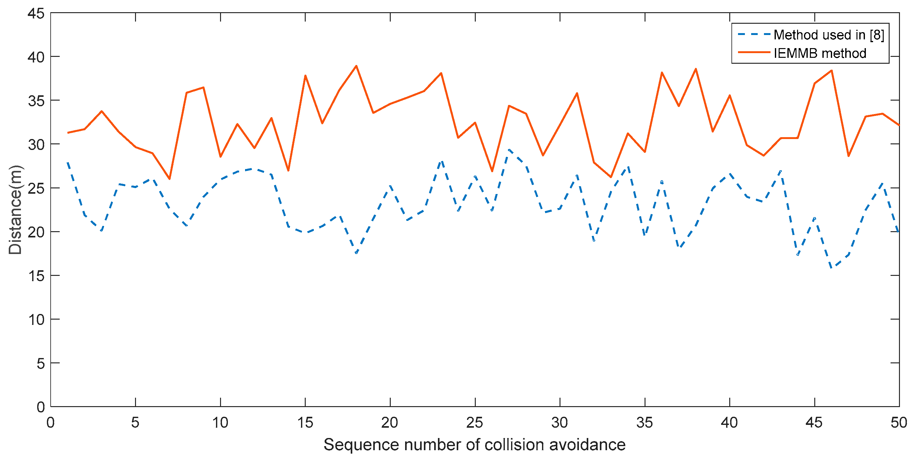
Figure 14.
Collision detection distance on winding roads. The detection distance of the IEMMB method on a winding road is longer than the method used in [8].
Figure 14.
Collision detection distance on winding roads. The detection distance of the IEMMB method on a winding road is longer than the method used in [8].

Figure 15.
Maximum yaw rate during collision avoidance.
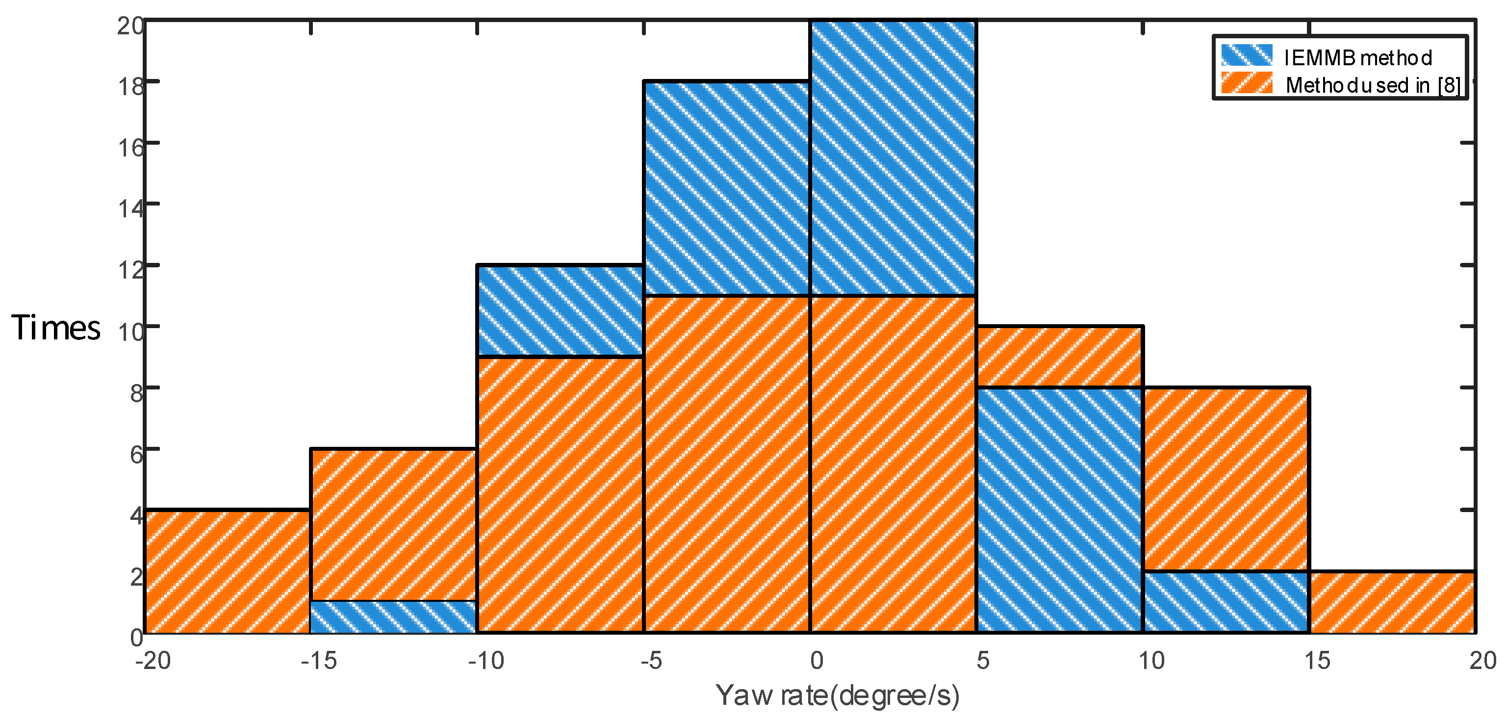
Figure 16.
Maximum acceleration during collision avoidance.

Figure 17.
Collision avoidance on a straight road. (a) Keep lane without collision point detected; (b) collision point is detected and represented with a red point; (c) a lane change path is generated to avoid the potential collision. Trajectories of detected vehicles are represented by yellow lines and the planned path of the autonomous vehicle is represented by a green line. The red numbers represent the sequence number of the processed data from sensors and the internal between two frames is 40 ms.

Figure 18.
Collision avoidance on a winding road. (a) A collision point is detected; (b) decelerate to avoid the collision; (c) avoid potential collision successfully. The red number represents the ID of the detected obstacle which is unique.
Figure 18.
Collision avoidance on a winding road. (a) A collision point is detected; (b) decelerate to avoid the collision; (c) avoid potential collision successfully. The red number represents the ID of the detected obstacle which is unique.

Figure 19.
Collision avoidance without intent estimation. (a) No collision is detected; (b) changing lane to avoid a collision which is represented with a red point; (c) avoiding a potential collision successfully. The green box represents the dynamic obstacle detection range of the three-dimensional LIDAR, and the area between the two green lines illustrates the detection area of the IBEO LIDAR. The planned trajectory of the autonomous vehicle is represented with a red line. The velocity and moving direction of detected obstacles are written in red besides the detected obstacles.


Table 1.
Means and standard deviations of feature vectors and two feature vector samples.
| Examples | |||
|---|---|---|---|
| 0.9 | −0.1 | 1.91 | |
| 0.40 | 1.76 | 0.69 | |
| Vector_1 (left lane change) | 1.1 | −0.8 | 1.6 |
| Vector_2 (normal moving) | 0.6 | 0.4 | 0.8 |
| Z-score of Vector_1 | 0.5 | −0.82 | 0.45 |
| Z-score of Vector_2 | −0.75 | 0.28 | −1.61 |
Table 2.
Data used in the training process.
| Maneuver Type | Normal Moving | Left Lane Change | Right Lane Change | |
|---|---|---|---|---|
| Road Type | ||||
| Straight Road | 50 | 50 | 50 | |
| Winding Road | 50 | 50 | 50 | |
Table 3.
Performance on straight roads.
| Methods | Intent Types | True Positive | False Positive | False Negative | Precision Rate | Recall Rate | F-Score |
|---|---|---|---|---|---|---|---|
| Proposed Method | Normal moving | 270 | 8 | 8 | 97.1% | 97.1% | 97.1% |
| Left lane changes | 34 | 5 | 4 | 87.2% | 89.5% | 88.6% | |
| Right lane change | 30 | 3 | 4 | 90.9% | 88.2% | 89.5% | |
| Method in [11] | Normal moving | 249 | 19 | 29 | 92.9% | 89.6% | 91.2% |
| Left lane change | 28 | 16 | 10 | 63.6% | 73.7% | 68.3% | |
| Right lane change | 25 | 13 | 9 | 65.8% | 73.5% | 69.4% |
Table 4.
Performance on winding roads.
| Methods | Intent Types | True Positive | False Positive | False Negative | Precision Rate | Recall Rate | F-Score |
|---|---|---|---|---|---|---|---|
| Proposed Method | Normal moving | 221 | 9 | 12 | 96.1% | 94.8% | 95.4% |
| Left lane changes | 33 | 7 | 5 | 82.5% | 86.8% | 84.6% | |
| Right lane change | 25 | 5 | 4 | 83.3% | 86.2% | 84.7% | |
| Method in [11] | Normal moving | 176 | 36 | 57 | 83.0% | 75.5% | 79.1% |
| Left lane change | 17 | 33 | 21 | 34% | 44.7% | 38.6% | |
| Right lane change | 14 | 24 | 15 | 36.8% | 48.3% | 41.8% |
© 2017 by the authors. Licensee MDPI, Basel, Switzerland. This article is an open access article distributed under the terms and conditions of the Creative Commons Attribution (CC BY) license (http://creativecommons.org/licenses/by/4.0/).
Share and Cite
MDPI and ACS Style
Huang, R.; Liang, H.; Zhao, P.; Yu, B.; Geng, X. Intent-Estimation- and Motion-Model-Based Collision Avoidance Method for Autonomous Vehicles in Urban Environments. Appl. Sci. 2017, 7, 457. https://doi.org/10.3390/app7050457
AMA Style
Huang R, Liang H, Zhao P, Yu B, Geng X. Intent-Estimation- and Motion-Model-Based Collision Avoidance Method for Autonomous Vehicles in Urban Environments. Applied Sciences. 2017; 7(5):457. https://doi.org/10.3390/app7050457
Chicago/Turabian StyleHuang, Rulin, Huawei Liang, Pan Zhao, Biao Yu, and Xinli Geng. 2017. "Intent-Estimation- and Motion-Model-Based Collision Avoidance Method for Autonomous Vehicles in Urban Environments" Applied Sciences 7, no. 5: 457. https://doi.org/10.3390/app7050457
Note that from the first issue of 2016, this journal uses article numbers instead of page numbers. See further details here.