
A Fast Motion Parameters Estimation Method Based on Cross-Correlation of Adjacent Echoes for Wideband LFM Radars

 ,
, 
Abstract
:1. Introduction
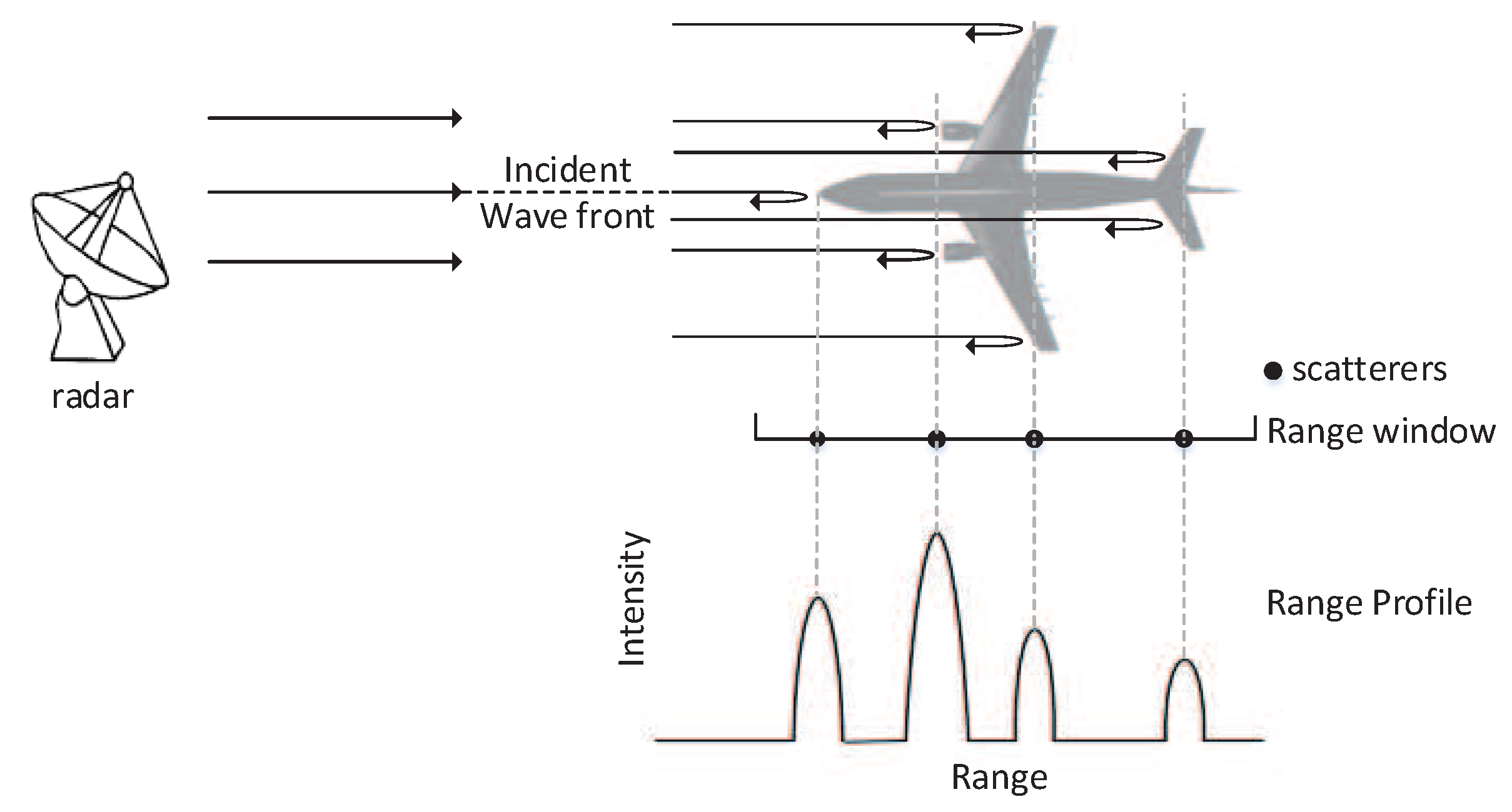
2. Signal Model
3. Estimation of Motion Parameters Based on the CCAE Method
3.1. “Stretching” Idea of the Proposed CCAE Method
3.2. Proposed CCAE Algorithm
3.2.1. Estimation of Velocity
3.2.2. Estimation of Higher Order Parameters
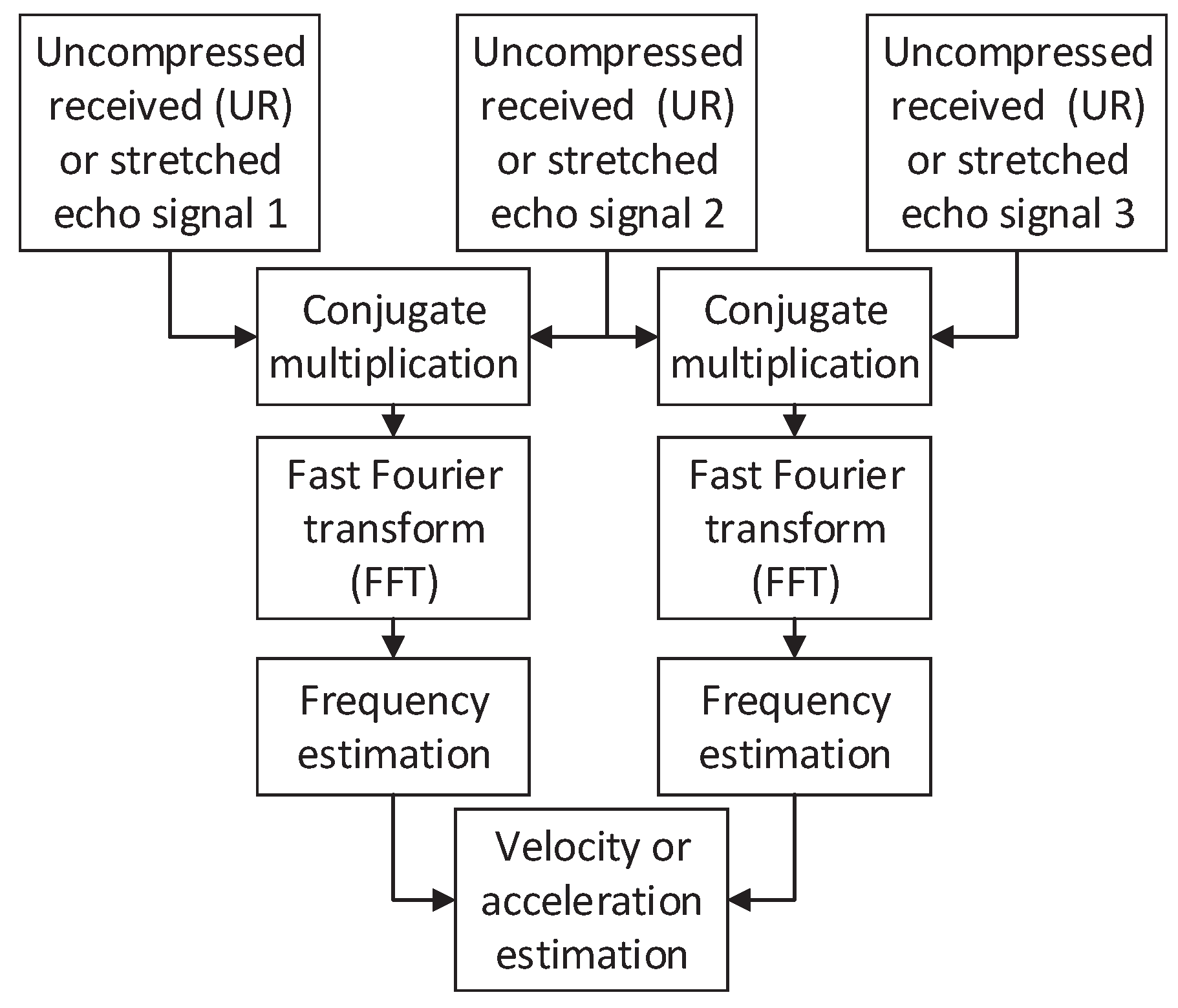
3.3. Implementation of the Proposed CCAE Method
- The first UR or stretched signal is multiplied with the conjugate of the second UR or stretched signal. For acceleration estimation, the second echo signal is also multiplied with the third echo signal.
- The FFT operation is performed on the multiplication results for energy accumulation.
- Estimate the frequencies of the above FFT results.
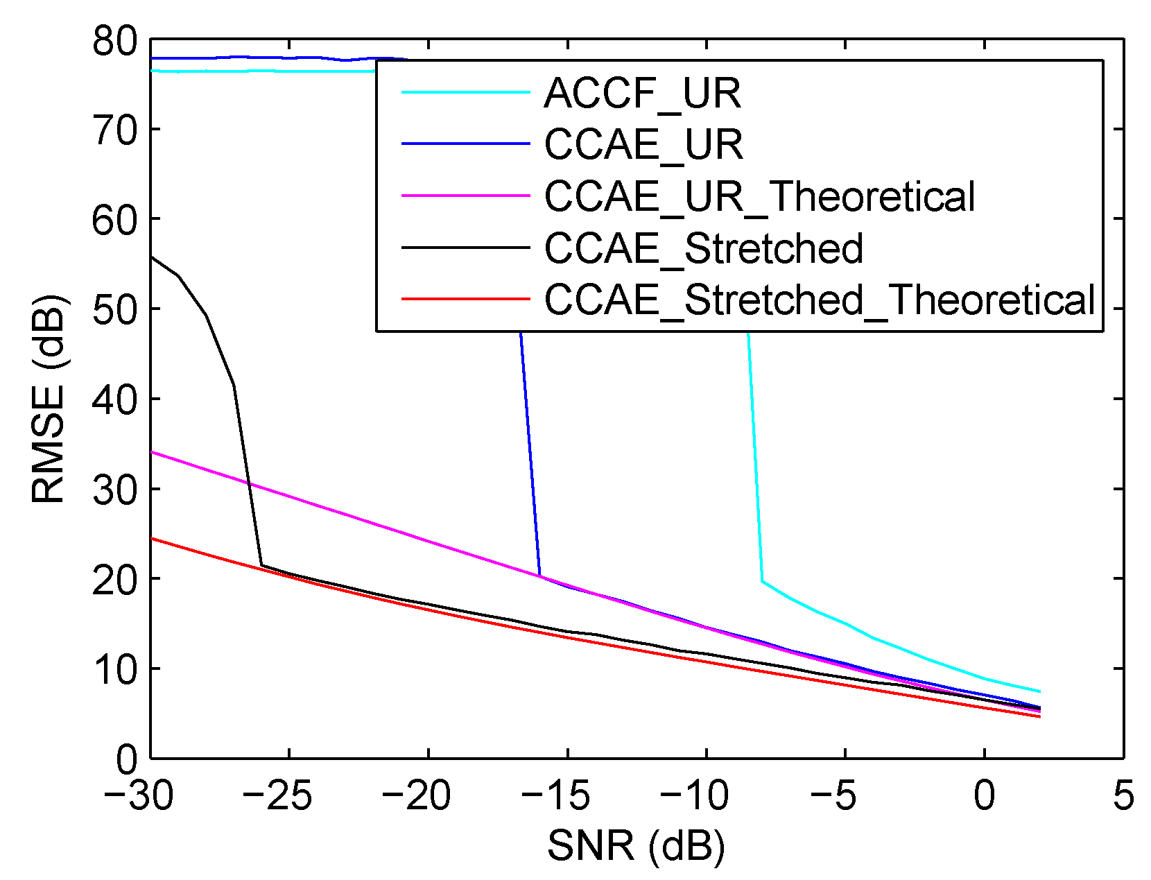
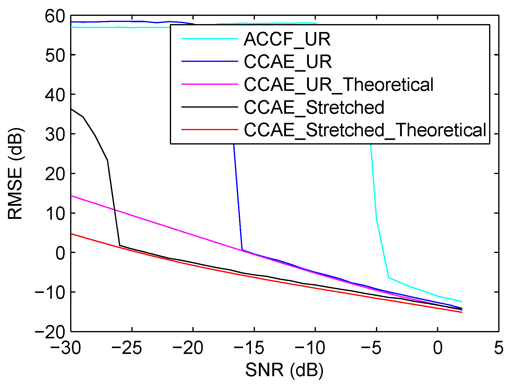
3.4. Performance Analysis
4. Simulations and Real Data Processing
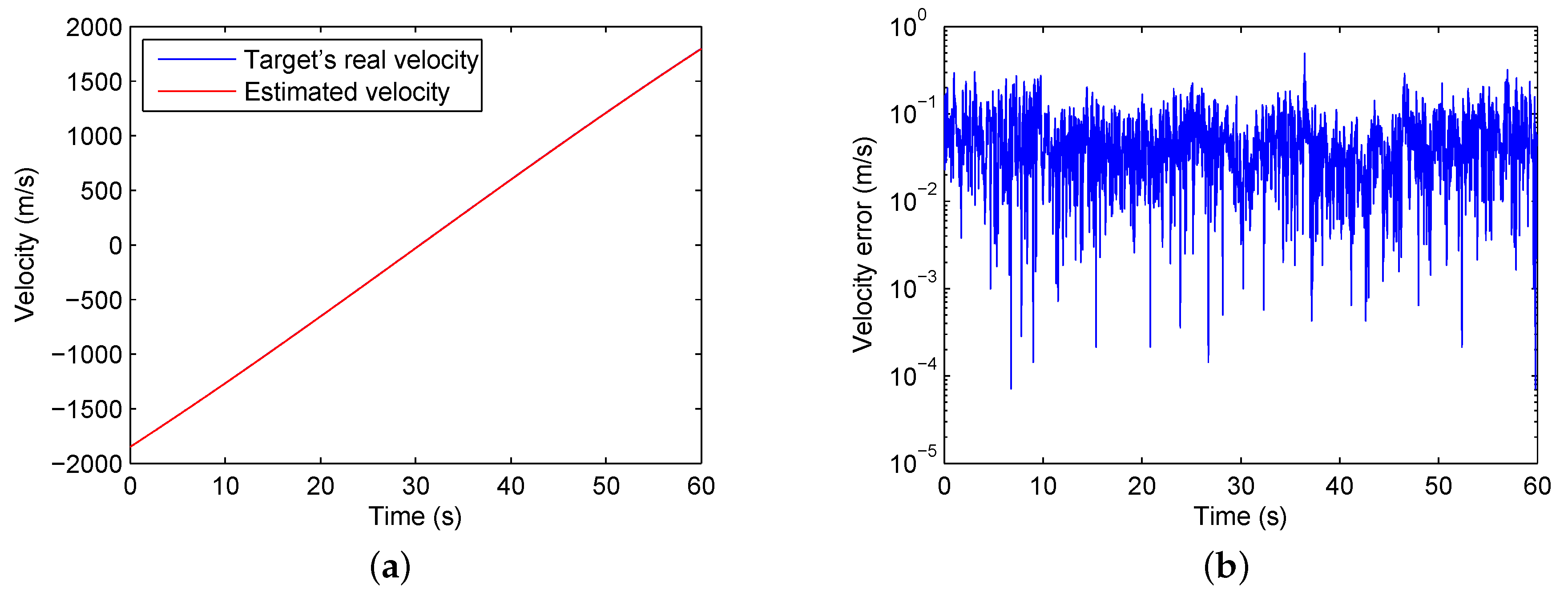
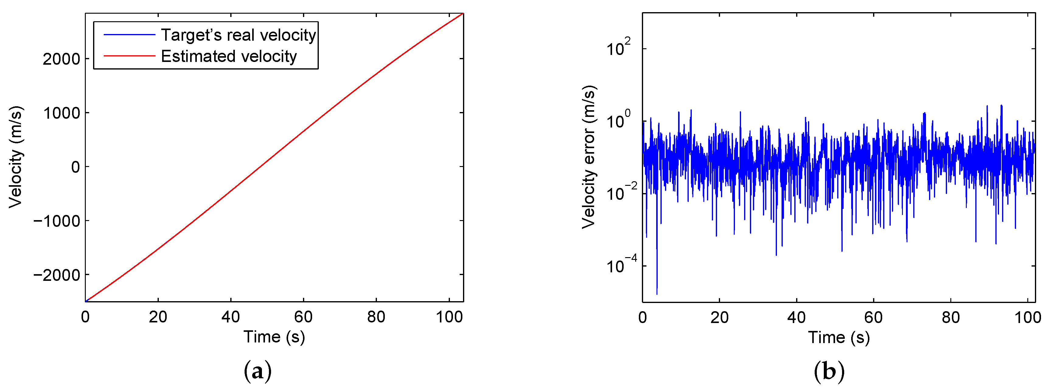
4.1. Evaluation of the Proposed CCAE Method
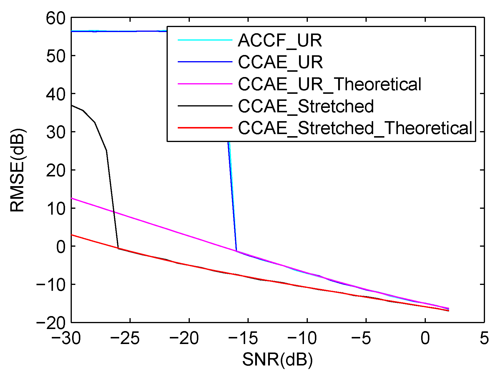
4.2. Comparison with the ACCF Method
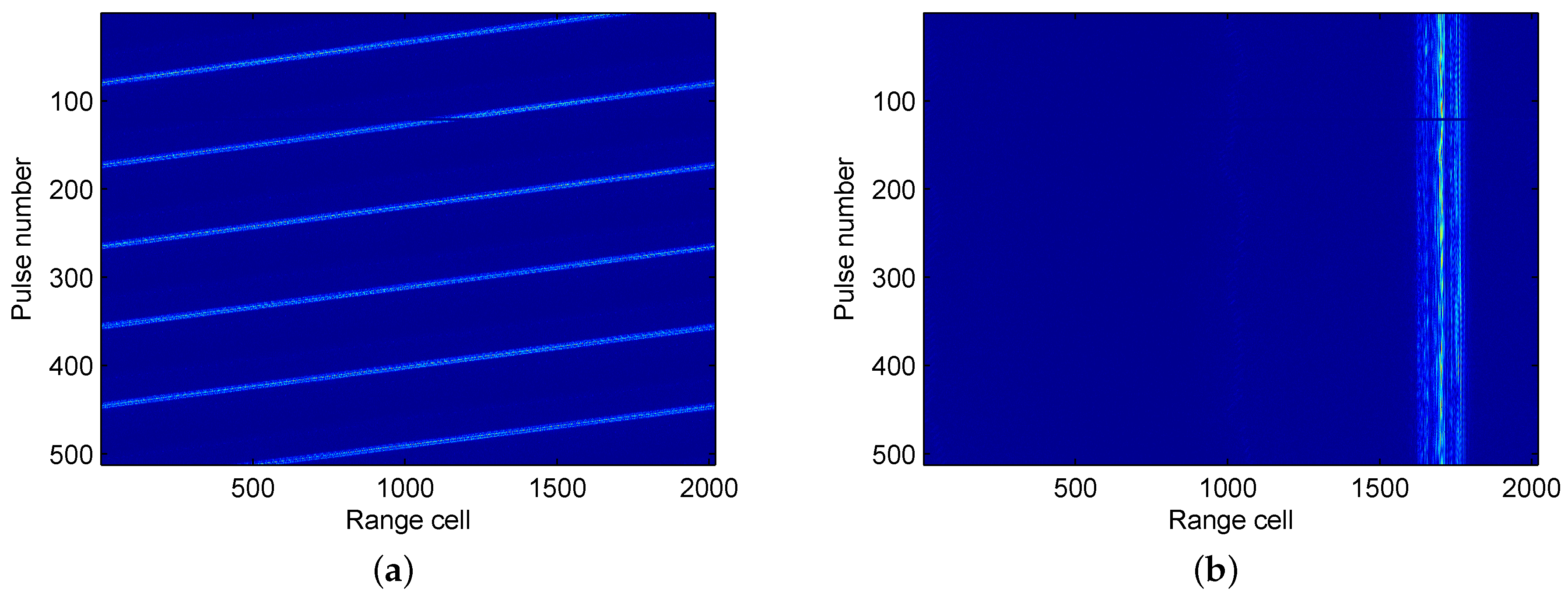
4.3. Verification with Real Data
5. Conclusions
Acknowledgments
Author Contributions
Conflicts of Interest
References
- Skolnik, M.I. Introduction to radar. In Radar Handbook; McGraw-Hill: New York, NY, USA, 1962. [Google Scholar]
- Berizzi, F.; Mese, E.D.; Diani, M.; Martorella, M. High-resolution ISAR imaging of maneuvering targets by means of the range instantaneous Doppler technique: Modeling and performance analysis. IEEE Trans. Image Process. 2001, 10, 1880–1890. [Google Scholar] [CrossRef] [PubMed]
- Suo, P.C.; Tao, S.; Tao, R.; Nan, Z. Detection of high-speed and accelerated target based on the linear frequency modulation radar. IET Radar Sonar Navig. 2014, 8, 37–47. [Google Scholar] [CrossRef]
- Wehner, D.R. High Resolution Radar; Artech House, Inc.: Norwood, MA, USA, 1987. [Google Scholar]
- Werness, S.A.; Carrara, W.G.; Joyce, L.; Franczak, D.B. Moving target imaging algorithm for SAR data. IEEE Trans. Aerosp. Electron. Syst. 1990, 26, 57–67. [Google Scholar] [CrossRef]
- Chen, V.C.; Qian, S. Joint time-frequency transform for radar range-Doppler imaging. IEEE Trans. Aerosp. Electron. Syst. 1998, 34, 486–499. [Google Scholar] [CrossRef]
- Peng, S.B.; Xu, J.; Peng, Y.N.; Xiang, J.B. Parametric inverse synthetic aperture radar manoeuvring target motion compensation based on particle swarm optimiser. IET Radar Sonar Navig. 2011, 5, 305–314. [Google Scholar] [CrossRef]
- Chen, C.C.; Andrews, H.C. Target-motion-induced radar imaging. IEEE Trans. Aerosp. Electron. Syst. 1980, 16, 2–14. [Google Scholar] [CrossRef]
- Yu, J.; Xu, J.; Peng, Y.N.; Xia, X.G. Radon-Fourier transform for radar target detection III: Optimality and fast implementations. IEEE Trans. Aerosp. Electron. Syst. 2012, 48, 991–1004. [Google Scholar] [CrossRef]
- Wang, Y.; Ling, H.; Chen, V.C. ISAR motion compensation via adaptive joint time-frequency technique. IEEE Trans. Aerosp. Electron. Syst. 1998, 34, 670–677. [Google Scholar] [CrossRef]
- Wang, J.; Kasilingam, D. Global range alignment for ISAR. IEEE Trans. Aerosp. Electron. Syst. 2003, 39, 351–357. [Google Scholar] [CrossRef]
- Li, J.; Wu, R.; Chen, V.C. Robust autofocus algorithm for ISAR imaging of moving targets. IEEE Trans. Aerosp. Electron. Syst. 2001, 37, 1056–1069. [Google Scholar]
- Wu, H.; Grenier, D.; Delisle, G.Y.; Fang, D.G. Translational motion compensation in ISAR image processing. IEEE Trans. Image Process. 1995, 4, 1561–1571. [Google Scholar] [PubMed]
- Xing, M.; Wu, R.; Lan, J.; Bao, Z. Migration through resolution cell compensation in ISAR imaging. IEEE Geosci. Remote Sens. Lett. 2004, 1, 141–144. [Google Scholar] [CrossRef]
- Son, J.S.; Thomas, G.; Flores, B. Range-Doppler Radar Imaging and Motion Compensation; Artech House: Norwood, MA, USA, 2001. [Google Scholar]
- Xi, L.; Guosui, L.; Ni, J. Autofocusing of ISAR images based on entropy minimization. IEEE Trans. Aerosp. Electron. Syst. 1999, 35, 1240–1252. [Google Scholar] [CrossRef]
- Xu, J.; Yu, J.; Peng, Y.N.; Xia, X.G. Radon-Fourier transform for radar target detection, I: Generalized Doppler filter bank. IEEE Trans. Aerosp. Electron. Syst. 2011, 47, 1186–1202. [Google Scholar] [CrossRef]
- Xu, J.; Xia, X.G.; Peng, S.B.; Yu, J.; Peng, Y.N.; Qian, L.C. Radar maneuvering target motion estimation based on generalized Radon-Fourier transform. IEEE Trans. Signal Process. 2012, 60, 6190–6201. [Google Scholar]
- Perry, R.; Dipietro, R.; Fante, R. SAR imaging of moving targets. IEEE Trans. Aerosp. Electron. Syst. 1999, 35, 188–200. [Google Scholar] [CrossRef]
- Zhu, D.; Li, Y.; Zhu, Z. A keystone transform without interpolation for SAR ground moving-target imaging. IEEE Geosci. Remote Sens. Lett. 2007, 4, 18–22. [Google Scholar] [CrossRef]
- Li, G.; Xia, X.G.; Peng, Y.N. Doppler keystone transform: An approach suitable for parallel implementation of SAR moving target imaging. IEEE Geosci. Remote Sens. Lett. 2008, 5, 573–577. [Google Scholar] [CrossRef]
- Zhu, D.; Wang, L.; Yu, Y.; Tao, Q.; Zhu, Z. Robust ISAR range alignment via minimizing the entropy of the average range profile. IEEE Geosci. Remote Sens. Lett. 2009, 6, 204–208. [Google Scholar]
- Li, Y.; Xing, M.; Su, J.; Quan, Y.; Bao, Z. A new algorithm of ISAR imaging for maneuvering targets with low SNR. IEEE Trans. Aerosp. Electron. Syst. 2013, 49, 543–557. [Google Scholar] [CrossRef]
- Li, X.; Cui, G.; Yi, W.; Kong, L. A fast maneuvering target motion parameters estimation algorithm based on ACCF. IEEE Signal Process. Lett. 2015, 22, 270–274. [Google Scholar] [CrossRef]
- Li, X.; Cui, G.; Kong, L.; Yi, W. Fast Non-Searching Method for Maneuvering Target Detection and Motion Parameters Estimation. IEEE Trans. Signal Process. 2016, 64, 2232–2244. [Google Scholar] [CrossRef]
- Lv, X.; Bi, G.; Wan, C.; Xing, M. Lv’s distribution: Principle, implementation, properties, and performance. IEEE Trans. Signal Process. 2011, 59, 3576–3591. [Google Scholar] [CrossRef]
- Luo, S.; Bi, G.; Lv, X.; Hu, F. Performance analysis on Lv distribution and its applications. Digit. Signal Process. 2013, 23, 797–807. [Google Scholar] [CrossRef]
- Li, X.; Kong, L.; Cui, G.; Yi, W.; Yang, Y. ISAR imaging of maneuvering target with complex motions based on ACCF–LVD. Digit. Signal Process. 2015, 46, 191–200. [Google Scholar] [CrossRef]
- Shui, P.L.; Xu, S.W.; Liu, H.W. Range-spread target detection using consecutive HRRPs. IEEE Trans. Aerosp. Electron. Syst. 2011, 47, 647–665. [Google Scholar] [CrossRef]
- Abatzoglou, T.J. A fast maximum likelihood algorithm for frequency estimation of a sinusoid based on Newton’s method. IEEE Trans. Acoust. Speech Signal Process. 1985, 33, 77–89. [Google Scholar] [CrossRef]
- Xia, X.G. A quantitative analysis of SNR in the short-time Fourier transform domain for multicomponent signals. IEEE Trans. Signal Process. 1998, 46, 200–203. [Google Scholar]
- Xia, X.G.; Chen, V.C. A quantitative SNR analysis for the pseudo Wigner-Ville distribution. IEEE Trans. Signal Process. 1999, 47, 2891–2894. [Google Scholar]
- O’Donoughue, N.; Moura, J.M.F. On the Product of Independent Complex Gaussians. IEEE Trans. Signal Process. 2012, 60, 1050–1063. [Google Scholar] [CrossRef]
- Ma, N.; Goh, J.T. Ambiguity-function-based techniques to estimate DOA of broadband chirp signals. IEEE Trans. Signal Process. 2006, 54, 1826–1839. [Google Scholar]
- Rife, D.; Boorstyn, R. Single tone parameter estimation from discrete-time observations. IEEE Trans. Inf. Theory 1974, 20, 591–598. [Google Scholar] [CrossRef]


| Notation | Type | Meaning |
|---|---|---|
| Subscript | The received signal is uncompressed. | |
| Subscript | The signal is stretched. | |
| Subscript | The signal is obtained by multiplying a echo signal with the conjugate of another echo signal. | |
| Subscript | The signal is the multiplication result of the different echo signal from the same scatterers. | |
| Subscript | The signal is the multiplication result of the different echo signal from the different scatterers. | |
| Signal | The transmitted signal. | |
| Signal | The local reference signal. | |
| Signal | The uncompressed received signal. | |
| Signal | The stretched signal. | |
| Signal | The distance from radar to the p-th scatterer. |
| Center Frequency (GHz) | Bandwidth (MHz) | Pulse Width (μs) | Sampling Frequency (MHz) | PRI (ms) |
|---|---|---|---|---|
| 9 | 200 | 100 | 10 | 5 |
| Center Frequency (GHz) | Bandwidth (GHz) | Pulse Width (μs) | Sampling Frequency (MHz) | PRI (ms) |
|---|---|---|---|---|
| 9 | 1 | 100 | 10 | 10 |
| Time Cost (s) | CCAE_Stretched | CCAE_UR | ACCF_UR |
|---|---|---|---|
| Estimation without acceleration | 81.6 | 2545.1 | 5282.1 |
| Estimation with acceleration | 156.5 | 4869.7 | 10175.3 |
| Parameters | Radar 1 | Radar 2 |
|---|---|---|
| Center Frequency (GHz) | 9 | 3.2 |
| Bandwidth (MHz) | 2000 | 300 |
| Sampling Frequency (MHz) | 10 | 10 |
| Pulse Width (μs) | 400 | 200 |
| PRI (ms) | 40 | 100 |
© 2017 by the authors. Licensee MDPI, Basel, Switzerland. This article is an open access article distributed under the terms and conditions of the Creative Commons Attribution (CC BY) license (http://creativecommons.org/licenses/by/4.0/).
Share and Cite
Zhang, Y.-X.; Hong, R.-J.; Yang, C.-F.; Zhang, Y.-J.; Deng, Z.-M.; Jin, S. A Fast Motion Parameters Estimation Method Based on Cross-Correlation of Adjacent Echoes for Wideband LFM Radars. Appl. Sci. 2017, 7, 500. https://doi.org/10.3390/app7050500
Zhang Y-X, Hong R-J, Yang C-F, Zhang Y-J, Deng Z-M, Jin S. A Fast Motion Parameters Estimation Method Based on Cross-Correlation of Adjacent Echoes for Wideband LFM Radars. Applied Sciences. 2017; 7(5):500. https://doi.org/10.3390/app7050500
Chicago/Turabian StyleZhang, Yi-Xiong, Ru-Jia Hong, Cheng-Fu Yang, Yun-Jian Zhang, Zhen-Miao Deng, and Sheng Jin. 2017. "A Fast Motion Parameters Estimation Method Based on Cross-Correlation of Adjacent Echoes for Wideband LFM Radars" Applied Sciences 7, no. 5: 500. https://doi.org/10.3390/app7050500
APA StyleZhang, Y.-X., Hong, R.-J., Yang, C.-F., Zhang, Y.-J., Deng, Z.-M., & Jin, S. (2017). A Fast Motion Parameters Estimation Method Based on Cross-Correlation of Adjacent Echoes for Wideband LFM Radars. Applied Sciences, 7(5), 500. https://doi.org/10.3390/app7050500