Sintering of Two Viscoelastic Particles: A Computational Approach

Abstract

Selective laser sintering (SLS) is a high-resolution additive manufacturing fabrication technique. To fully understand the process, we developed a computational model, using the finite element method, to solve the flow problem of sintering two viscoelastic particles. The flow is assumed to be isothermal and the particles to be in a liquid state, where their rheology is described using the Giesekus and XPP constitutive models. In this work, we assess the parameters that define this problem, such as the initial geometry, the Deborah number and other dimensionless parameters present in the rheological models. In particular, the conformation tensor is considered, which is a measure for the polymeric strain and plays an important role in the crystallization kinetics of semicrystalline polymers like polyamide 12, usually used in SLS.

1. Introduction

Sintering can be described as the process where material particles are fused together by heat or pressure, without fully melting the material. Materials like metals, ceramics, glass and polymers can be used in this process. In viscous sintering, capillary forces act to minimize the surface area, where the surface tension is the driving force of the flow. Sintering of polymer powder is the basis of selective laser sintering (SLS), an additive manufacturing technique. SLS is a professional fabrication technique, since it enables the production of almost any shape or geometry. To fully exploit the possibilities, we need to understand the sintering process and the accompanying material aspects in detail.

Frenkel [1] was the first to give an analytical solution for the shape evolution of two spherical particles during coalescence. This model uses a mechanical energy balance, where the work done by the surface tension is in balance with the work done by viscous dissipation and is limited by the early stages of sintering. Eshelby [2] corrected this model for continuity, assuming biaxial extensional flow. Pokluda et al. [3] improved the corrected model by taking the change in particle radius into account. To describe the sintering of viscoelastic particles, Bellehumeur et al. [4] extended Frenkel’s approach with the steady-state upper-convected Maxwell (UCM) constitutive model, and Scribben et al. [5] continued this work by describing the transient viscoelastic coalescence of two particles using UCM.

Hopper [6] found an analytical solution for the time evolution of viscous planar flow in a region bounded by a smooth closed curve, driven by surface tension. His work includes the coalescence of two equally-sized cylinders. Richardson [7] extended this for geometries of two unequal cylinders. The work of Crowdy [8] gives exact solutions for the surface evolution of planar multiply-connected domains, including geometries with different particle sizes and pores.

Bellehumeur et al. [9] conducted sintering experiments using different commercial rotational molding-grade resins of high-density polyethylene and linear low-density polyethylene. Hopper’s model predicted the experimental data well, but underestimated the time required for the completion of coalescence. From experiments with acrylic resins, Mazur and Plazek [10] found that models based on Newtonian viscous flows underestimate the initial coalescence rate for this type of polymer, since in the early sintering stages, the deformation is quasi-elastic. Scribben et al. [5] compared their transient UCM model with experiments on isotactic polypropylenes and showed that the model improves the accuracy at short time scales, but does not decrease the error at long time scales.

Towards the computational modeling of viscous sintering, Ross et al. [11] developed a dynamic model of the sintering process of an infinite line of cylinders using the finite element method. The boundary element method was applied by Kuiken [12] to simulate how a moderately curved initial two-dimensional shape transforms itself into a circle, and Van de Vorst [13] used this method to solve a two-dimensional Stokes problem for multiply-connected domains in which the pores can shrink and disappear. Martínez-Herrera and Derby [14] used the finite element method to assess the two-dimensional viscous sintering of particles with different initial ratios of particle radii. Three-dimensional modeling is done by Jagota and Dawson [15,16] using the finite element method, assuming axisymmetry. Furthermore, both Van de Vorst [17] and Martínez-Herrera and Derby [18] extended their original two-dimensional models to axisymmetric problems. Zhou and Derby [19] developed a fully three-dimensional finite element model for viscous sintering. Hooper et al. [20] developed a model using the finite element method to study the sintering of viscoelastic particles using the UCM model. In their work, the initial conditions are chosen to be the quasi-steady-state velocity profile, compatible pressure and extra-stress fields, obtained by solving the conservation equations with all time derivatives set to zero while holding the boundary fixed.

In this work, we study the flow problem of the sintering of polymeric particles with a fully-transient viscoelastic finite element method. We assess the importance of the initial geometry, the Deborah number and other dimensionless parameters present in both the Giesekus and the eXtended Pom-Pom (XPP) constitutive model, all in an axisymmetric geometry of two spherical particles.

2. Problem Description

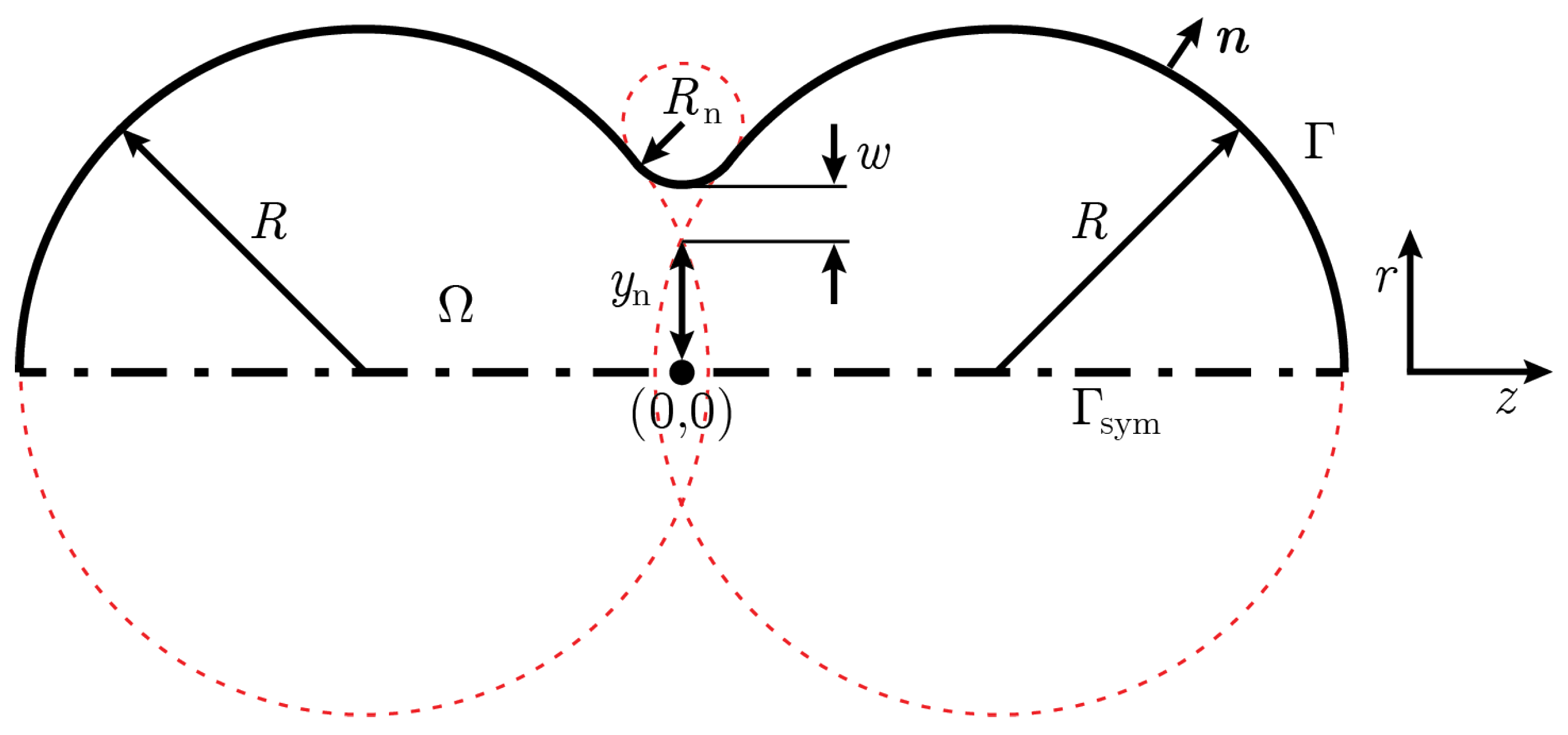
We consider two evenly-sized liquid polymer particles that are initially connected to each other by a neck. The initial geometry ${\mathsf{\Omega }}_{t=0}$ is given in Figure 1. The outer surface of the geometry is $\mathrm{\Gamma }$, with $\mathit{n}$ the outwardly-directed unit normal vector. The geometry is assumed to be axisymmetric, where the axial coordinate is denoted by z and the radial coordinate by r, using the convention $(z,r)$. The symmetry axis is given by ${\mathrm{\Gamma }}_{\mathrm{sym}}$. The radii of the particles R, together with the initial contact radius $y_{\mathrm{n}}$, define the initial geometry. To avoid discontinuities in the slope of the interface, the parameter $R_{\mathrm{n}}=R\times {(y_{\mathrm{n}}/R)}^3$ [20] rounds off the neck region. Due to the round off by $R_{\mathrm{n}}$, the real initial contact radius becomes $y_{t=0}=y_{\mathrm{n}}+w$. These two liquid particles will merge into one larger sphere with radius $R_{\mathrm{final}}$, determined by the initial volume of the geometry, under the influence of the surface tension prescribed on surface $\mathrm{\Gamma }$.

Figure 1. Geometry ${\mathsf{\Omega }}_{t=0}$ of the two liquid polymer particles.

3. Governing Equations

3.1. Balance Equations and Constitutive Models

The flow behavior of the sintering process of polymer particles as introduced in the previous section, assuming an isothermal flow, can be described using the momentum and mass balance. We assume the fluid to be incompressible, leading to the following set of equations:

$$\begin{array}{cc}\hfill \rho {\displaystyle \frac{\mathrm{D}\mathit{u}}{\mathrm{D}t}}=\nabla ·\mathit{\sigma }+\rho g{\mathit{e}}_{\mathrm{g}}& \mathrm{in}\mathsf{\Omega },\end{array}$$

(1)

$$\begin{array}{cc}\hfill \nabla ·\mathit{u}=0& \mathrm{in}\mathsf{\Omega },\end{array}$$

(2)

where $\mathrm{D}\left(\right)/\mathrm{D}t$ denotes the material derivative, $\rho$ is the fluid density, $\mathit{u}$ the fluid velocity, $\mathit{\sigma }$ the Cauchy stress tensor and g and ${\mathit{e}}_{\mathrm{g}}$ the magnitude and direction of gravity, respectively. For the Newtonian constitutive equation, the Cauchy stress tensor is:

$$\mathit{\sigma }=-p\mathit{I}+\mu \left(\nabla \mathit{u}+{(\nabla \mathit{u})}^{\mathrm{T}}\right).$$

(3)

Herein, p is the pressure and $\mu$ the viscosity. For viscoelastic fluids, the Cauchy stress tensor can be written as:

$$\mathit{\sigma }=-p\mathit{I}+{\eta }_{\mathrm{s}}\left(\nabla \mathit{u}+{(\nabla \mathit{u})}^{\mathrm{T}}\right)+\mathit{\tau },$$

(4)

with the viscoelastic extra-stress tensor $\mathit{\tau }$ written in the conformation tensor form:

$$\mathit{\tau }=G(\mathit{c}-\mathit{I}),$$

(5)

where ${\eta }_{\mathrm{s}}$ is the solvent viscosity and G the modulus. For the Giesekus constitutive equation, the evolution of the conformation tensor $\mathit{c}$ is described by:

$$\lambda \stackrel{▿}{\mathit{c}}+\mathit{c}-\mathit{I}+\alpha {(\mathit{c}-\mathit{I})}^2=\mathbf{0}.$$

(6)

Herein, $\stackrel{▿}{\left(\right)}=\mathrm{D}\left(\right)/\mathrm{D}t-{(\nabla \mathit{u})}^{\mathrm{T}}·\left(\right)-\left(\right)·\nabla \mathit{u}$ denotes the upper-convected derivative, $\lambda$ the relaxation time and $\alpha$ the material parameter defining the amount of anisotropy. For the XPP model [21], the evolution of the conformation tensor $\mathit{c}$ is given by:

$$\stackrel{▿}{\mathit{c}}+2{\displaystyle \frac{\exp [\nu \sqrt{\mathrm{tr}\left(\mathit{c}\right)/3}-1]}{{\lambda }_{\mathrm{s}}}}\left(1-{\displaystyle \frac{3}{\mathrm{tr}\left(\mathit{c}\right)}}\right)\mathit{c}+{\displaystyle \frac{1}{\lambda }}\left({\displaystyle \frac{3\mathit{c}}{\mathrm{tr}\left(\mathit{c}\right)}}-\mathit{I}\right)=\mathbf{0},$$

(7)

where $\nu =2/q$ with q the number of arms at the end of the backbone, ${\lambda }_{\mathrm{s}}$ the relaxation time for the stretch and $\lambda$ the relaxation time of the backbone orientation.

The conformation tensor $\mathit{c}$ is, besides the velocity $\mathit{u}$ and pressure p, the third unknown to be solved as a function of position and time.

3.2. Interface Tracking

The motion of the surface $\mathrm{\Gamma }$ is tracked in a Lagrangian way, where the velocity of the surface is defined as:

$${\displaystyle \frac{d{\mathit{x}}_{\mathrm{\Gamma }}}{dt}}=\mathit{u}.$$

(8)

Herein, ${\mathit{x}}_{\mathrm{\Gamma }}$ is the function that maps the curvilinear coordinates onto the spatial coordinates of the surface, and $\mathit{u}$ is the material velocity at the surface $\mathrm{\Gamma }$.

3.3. Boundary Conditions

Along the surface $\mathrm{\Gamma }$ of the fluid, as shown in Figure 1, a constant surface tension $\gamma$ is prescribed using a Neumann boundary condition:

$$\begin{array}{cc}\hfill \mathit{\sigma }·\mathit{n}={\nabla }_{\mathrm{s}}·\left(\gamma {\mathit{I}}_{\mathrm{s}}\right)-p_{\mathrm{out}}\mathit{n}& \mathrm{on}\mathrm{\Gamma }.\end{array}$$

(9)

Herein, ${\nabla }_{\mathrm{s}}$ is the surface gradient operator, ${\mathit{I}}_{\mathrm{s}}=\mathit{I}-\mathit{nn}$ the second-order unit surface dyadic tensor and the outside pressure $p_{\mathrm{out}}$. For a more complex interfacial rheology, the current framework can be adjusted [22]. In the following, we assume $p_{\mathrm{out}}=0$. To impose symmetry, the velocity in the radial direction at the symmetry axis ${\mathrm{\Gamma }}_{\mathrm{sym}}$ is set to zero:

$$\begin{array}{cc}\hfill u_r=0& \mathrm{on}{\mathrm{\Gamma }}_{\mathrm{sym}}.\end{array}$$

(10)

Finally, the origin $(0,0)$ is fixed to prevent rigid body motion along the z-axis:

$$\begin{array}{cc}\hfill u_z=0& \mathrm{at}(0,0).\end{array}$$

(11)

Furthermore, to solve the system for a viscoelastic fluid, we initially apply a zero polymer stress to the system by prescribing ${\mathit{c}}_{t=0}=\mathit{I}$.

3.4. Dimensionless Equations

To scale the governing equations, we introduce characteristic constant values from the problem parameters. We define the characteristic length as $x_{\mathrm{c}}=R$, the characteristic velocity as $u_{\mathrm{c}}=\gamma /{\eta }_0$, the characteristic stress as ${\sigma }_{\mathrm{c}}=\gamma /R$, the characteristic pressure as $p_{\mathrm{c}}=\gamma /R$ and a characteristic time $t_{\mathrm{c}}$. Herein, ${\eta }_0$ is the zero-strain rate viscosity and is defined as ${\eta }_0=\mu$ for Newtonian fluids and ${\eta }_0={\eta }_{\mathrm{s}}+{\eta }_{\mathrm{p}}$ for viscoelastic fluids, where ${\eta }_{\mathrm{p}}=G\lambda$ is the polymer viscosity. A dimensionless variable can be obtained by dividing the original variable by the characteristic value, for example:

$$x^{*}={\displaystyle \frac{x}{x_{\mathrm{c}}}}={\displaystyle \frac{x}{R}}.$$

(12)

The dimensionless variable is represented by an asterisk superscript.

Scaling the boundary condition of Equation (8) leads to:

$${\displaystyle \frac{d{\mathit{x}}_{\mathrm{\Gamma }}^{*}R}{d{t}^{*}{t}_{\mathrm{c}}}}={\mathit{u}}^{*}{\displaystyle \frac{{\eta }_0}{\gamma }}.$$

(13)

Since both sides are assumed to be of the same order of magnitude, a definition for the characteristic time $t_{\mathrm{c}}=R{\eta }_0/\gamma$ follows, and Equation (13) reduces to:

$${\displaystyle \frac{d{\mathit{x}}_{\mathrm{\Gamma }}^{*}}{d{t}^{*}}}={\mathit{u}}^{*}.$$

(14)

Scaling the governing Equations (1) and (2) leads to:

$$\begin{array}{cc}\hfill \mathrm{La}{\displaystyle \frac{\mathrm{D}{\mathit{u}}^{*}}{\mathrm{D}{t}^{*}}}={\nabla }^{*}·{\mathit{\sigma }}^{*}+\mathrm{Bo}{\mathit{e}}_{\mathrm{g}}& \mathrm{in}\mathsf{\Omega },\end{array}$$

(15)

$$\begin{array}{cc}\hfill {\nabla }^{*}·{\mathit{u}}^{*}=0& \mathrm{in}\mathsf{\Omega },\end{array}$$

(16)

respectively. The two dimensionless numbers defining this flow problem are the Laplace number $\mathrm{La}=\rho \gamma R/{\eta }_0^2$, which is the ratio of the surface tension to the inertial forces, and the Bond number $\mathrm{Bo}=\rho R^{2}g/\gamma$, which is a measure of the gravity forces versus the surface tension forces. Both of these dimensionless numbers are negligibly small if we use the material parameters of polyamide 12 (PA12) powder (Table 1), which is most often used in SLS, i.e., $\mathrm{La}=\mathcal{O}\left({10}^{-8}\right)$ and $\mathrm{Bo}=\mathcal{O}\left({10}^{-3}\right)$. Equation (15) reduces to:

$$\begin{array}{cc}\hfill -{\nabla }^{*}·{\mathit{\sigma }}^{*}=\mathbf{0}& \mathrm{in}\mathsf{\Omega }.\end{array}$$

(17)

Table 1. Material properties of polyamide 12 (PA12) powder for SLS at $T=175{}^{\circ }\mathrm{C}$ (melt).

Parameter	Symbol	Value	References
Density	$\rho$	$\mathcal{O}\left(840\right)\mathrm{kg}/{\mathrm{m}}^3$	[23,24]
Viscosity	${\eta }_0$	$\mathcal{O}\left(400\right)\mathrm{Pa}$·s	[25]
Surface tension	$\gamma$	$\mathcal{O}\left(0.03\right)\mathrm{N}/\mathrm{m}$	[24,25]
Relaxation time	$\lambda$	$\mathcal{O}\left(0.05\right)\mathrm{s}$	[25]
Particle radius	R	$\mathcal{O}(3\times {10}^{-5})\mathrm{m}$	[25]

For the Newtonian case, the scaled Cauchy stress tensor Equation (3) is:

$${\mathit{\sigma }}^{*}=-p^{*}\mathit{I}+\left({\nabla }^{*}{\mathit{u}}^{*}+{\left({\nabla }^{*}{\mathit{u}}^{*}\right)}^{\mathrm{T}}\right).$$

(18)

Scaling the Cauchy stress tensor of viscoelastic fluids Equation (4) leads to:

$${\mathit{\sigma }}^{*}=-p^{*}\mathit{I}+\beta \left({\nabla }^{*}{\mathit{u}}^{*}+{\left({\nabla }^{*}{\mathit{u}}^{*}\right)}^{\mathrm{T}}\right)+{\mathit{\tau }}_{\mathrm{p}}^{*},$$

(19)

where $\beta ={\eta }_{\mathrm{s}}/{\eta }_0$. In this work, we choose $\beta =0.01$. The dimensionless description of Equation (6), the evolution of the conformation tensor $\mathit{c}$ for the Giesekus constitutive equation, is:

$$\mathrm{De}\stackrel{▿}{\mathit{c}}+\mathit{c}-\mathit{I}+\alpha {(\mathit{c}-\mathit{I})}^2=\mathbf{0}.$$

(20)

Besides the material parameter $\alpha$, we find the Deborah number $\mathrm{De}=\lambda \gamma /\left({\eta }_{0}R\right)$ in Equation (20), which is the ratio of the time scale of the fluid response to that of the process. For the XPP model, the dimensionless description of Equation (7) is:

$$\mathrm{De}\stackrel{▿}{\mathit{c}}+2\xi \exp [\nu \sqrt{\mathrm{tr}\left(\mathit{c}\right)/3}-1]\left(1-{\displaystyle \frac{3}{\mathrm{tr}\left(\mathit{c}\right)}}\right)\mathit{c}+\left({\displaystyle \frac{3\mathit{c}}{\mathrm{tr}\left(\mathit{c}\right)}}-\mathit{I}\right)=\mathbf{0}.$$

(21)

The dimensionless groups in Equation (21) are the Deborah number De as defined before, the ratio between the relaxation time of the backbone orientation and that of the stretch $\xi =\lambda /{\lambda }_{\mathrm{s}}$ and $\nu$, which depends on the number of arms q.

For the readability of this document, we omit the asterisks in the notation of the dimensionless variables.

4. Numerical Method

4.1. Moving Domain

To capture the motion of the moving domain $\mathsf{\Omega }$, the position of the surface $\mathrm{\Gamma }$ is predicted from previous time steps using:

$${\widehat{\mathit{x}}}_{\mathrm{\Gamma }}^{n+1}={\mathit{x}}_{\mathrm{\Gamma }}^n,$$

(22)

for the first time step and:

$${\widehat{\mathit{x}}}_{\mathrm{\Gamma }}^{n+1}=2{\mathit{x}}_{\mathrm{\Gamma }}^n-{\mathit{x}}_{\mathrm{\Gamma }}^{n-1},$$

(23)

for all subsequent time steps. Herein, ${\widehat{\mathit{x}}}_{\mathrm{\Gamma }}^{n+1}$ is the prediction of the surface position for time $t^{n+1}$, and ${\mathit{x}}_{\mathrm{\Gamma }}^n$ and ${\mathit{x}}_{\mathrm{\Gamma }}^{n-1}$ are the surface positions at time $t^n$ and $t^{n-1}$, respectively.

Next, the displacement of the fluid mesh is calculated from the surface displacement using a Laplace equation [26]. For the first time step, the mesh velocity in each node is calculated using a first-order backwards differencing scheme,

$${\mathit{u}}_{\mathrm{m}}^{n+1}={\displaystyle \frac{{\mathit{x}}_{\mathrm{m}}^{n+1}-{\mathit{x}}_{\mathrm{m}}^n}{\Delta t}},$$

(24)

whereas for subsequent time steps, a second-order backwards differencing scheme is used:

$${\mathit{u}}_{\mathrm{m}}^{n+1}={\displaystyle \frac{\frac{3}{2}{\mathit{x}}_{\mathrm{m}}^{n+1}-2{\mathit{x}}_{\mathrm{m}}^n+\frac{1}{2}{\mathit{x}}_{\mathrm{m}}^{n-1}}{\Delta t}}.$$

(25)

Herein, ${\mathit{u}}_{\mathrm{m}}^{n+1}$ is the mesh velocity at time $t^{n+1}$, and ${\mathit{x}}_{\mathrm{m}}^{n+1}$, ${\mathit{x}}_{\mathrm{m}}^n$ and ${\mathit{x}}_{\mathrm{m}}^{n-1}$ are the mesh coordinates at time $t^{n+1}$, $t^n$ and $t^{n-1}$, respectively.

Subsequently, the governing equations and boundary conditions are discretized on the newly-defined domain $\mathsf{\Omega }$. The momentum and mass balance are multiplied with the test functions $\mathit{v}$ and q in the appropriate function spaces:

$$\begin{array}{cc}\hfill \left(\mathit{v},-\nabla ·\mathit{\sigma }\right)=\mathbf{0},& \mathrm{for}\mathrm{all}\mathit{v},\end{array}$$

(26)

$$\begin{array}{cc}\hfill \left(q,\nabla ·\mathit{u}\right)=0,& \mathrm{for}\mathrm{all}q.\end{array}$$

(27)

Note that $\left(·,·\right)$ defines the inner product on $\mathsf{\Omega }$. Using partial integration and Gauss’ theorem, we obtain:

$$\begin{array}{cc}\hfill \left({(\nabla \mathit{v})}^{\mathrm{T}},\mathit{\sigma }\right)={\left(\mathit{v},\mathit{\sigma }·\mathit{n}\right)}_{\mathrm{\Gamma }},& \mathrm{for}\mathrm{all}\mathit{v},\end{array}$$

(28)

$$\begin{array}{cc}\hfill \left(q,\nabla ·\mathit{u}\right)=0,& \mathrm{for}\mathrm{all}q.\end{array}$$

(29)

Herein, ${\left(·,·\right)}_{\mathrm{\Gamma }}$ defines the inner product on $\mathrm{\Gamma }$. The right-hand side of Equation (28) can be filled using Equation (9), which is rewritten using partial integration and Weatherburn’s surface divergence theorem [27],

$$\begin{array}{cc}\hfill {\left(\mathit{v},\mathit{\sigma }·\mathit{n}\right)}_{\mathrm{\Gamma }}=-{\left({\left({\nabla }_{\mathrm{s}}\mathit{v}\right)}^{\mathrm{T}},\gamma {\mathit{I}}_{\mathrm{s}}\right)}_{\mathrm{\Gamma }}+{\left(({\nabla }_{\mathrm{s}}·\mathit{n})\mathit{n},\gamma {\mathit{I}}_{\mathrm{s}}·\mathit{v}\right)}_{\mathrm{\Gamma }}+{\left(\mathit{b},\gamma {\mathit{I}}_{\mathrm{s}}·\mathit{v}\right)}_{\partial \mathrm{\Gamma }},& \mathrm{for}\mathrm{all}\mathit{v},\end{array}$$

(30)

where $\mathit{b}=\mathit{t}\times \mathit{n}$ is the binormal and ${\left(·,·\right)}_{\partial \mathrm{\Gamma }}$ defines the inner product on the boundary of the surface $\partial \mathrm{\Gamma }$, i.e., the locations where the surface $\mathrm{\Gamma }$ meets the symmetry axis ${\mathrm{\Gamma }}_{\mathrm{sym}}$. Since the surface tension always acts tangential to the surface, $\mathit{n}·\gamma {\mathit{I}}_{\mathrm{s}}=0$. Furthermore, due to the area being zero on $\partial \mathrm{\Gamma }$, ${\left(\mathit{b},\gamma {\mathit{I}}_{\mathrm{s}}·\mathit{v}\right)}_{\partial \mathrm{\Gamma }}=0$. This leads to the following weak form:

$$\begin{array}{cc}\hfill \left({(\nabla \mathit{v})}^{\mathrm{T}},\mathit{\sigma }\right)=-{\left({\left({\nabla }_{\mathrm{s}}\mathit{v}\right)}^{\mathrm{T}},\gamma {\mathit{I}}_{\mathrm{s}}\right)}_{\mathrm{\Gamma }},& \mathrm{for}\mathrm{all}\mathit{v},\end{array}$$

(31)

$$\begin{array}{cc}\hfill \left(q,\nabla ·\mathit{u}\right)=0,& \mathrm{for}\mathrm{all}q.\end{array}$$

(32)

Next, we enter the Cauchy stress tensor into the weak formulation of the momentum balance. For the Newtonian fluid, the weak form is discretized according to the Galerkin approach and becomes: find $\mathit{u}$ and p, such that:

$$\begin{array}{cc}\hfill \left({(\nabla \mathit{v})}^{\mathrm{T}},2\mu \mathit{D}\right)-\left(\nabla ·\mathit{v},p\right)=-{\left({\left({\nabla }_{\mathrm{s}}\mathit{v}\right)}^{\mathrm{T}},\gamma {\mathit{I}}_{\mathrm{s}}\right)}_{\mathrm{\Gamma }},& \mathrm{for}\mathrm{all}\mathit{v},\end{array}$$

(33)

$$\begin{array}{cc}\hfill \left(q,\nabla ·\mathit{u}\right)=0,& \mathrm{for}\mathrm{all}q,\end{array}$$

(34)

using appropriate spaces for $\mathit{u}$, p, $\mathit{v}$ and q. Herein, $\mathit{D}=(\nabla \mathit{u}+{(\nabla \mathit{u})}^{\mathrm{T}})/2$. For both viscoelastic constitutive models, we employ the DEVSS-Gscheme [28,29,30] for stability. The SUPGmethod [31] and the log-conformation approach [32,33] are used to describe the evolution equation for the conformation tensor. The weak form becomes: find $\mathit{u}$, p, $\mathit{s}$ and $\mathit{G}$, such that:

$$\begin{array}{cc}\hfill \left({(\nabla \mathit{v})}^{\mathrm{T}},2{\eta }_{\mathrm{s}}\mathit{D}+\theta (\nabla \mathit{u}-{\mathit{G}}^{\mathrm{T}})+\mathit{\tau }\right)-\left(\nabla ·\mathit{v},p\right)=-{\left({\left({\nabla }_{\mathrm{s}}\mathit{v}\right)}^{\mathrm{T}},\gamma {\mathit{I}}_{\mathrm{s}}\right)}_{\mathrm{\Gamma }},& \mathrm{for}\mathrm{all}\mathit{v},\end{array}$$

(35)

$$\begin{array}{cc}\hfill \left(q,\nabla ·\mathit{u}\right)=0,& \mathrm{for}\mathrm{all}q,\end{array}$$

(36)

$$\begin{array}{cc}\hfill \left(\mathit{d}+\tau (\mathit{u}-{\mathit{u}}_{\mathrm{m}})·\nabla \mathit{d},{\displaystyle \frac{\mathrm{D}\mathit{s}}{\mathrm{D}t}}-\mathit{h}\left({(\nabla \mathit{u})}^{\mathrm{T}},\mathit{s}\right)\right)=\mathbf{0},& \mathrm{for}\mathrm{all}\mathit{d},\end{array}$$

(37)

$$\begin{array}{cc}\hfill \left(\mathit{H},-\nabla \mathit{u}+{\mathit{G}}^{\mathrm{T}}\right)=\mathbf{0},& \mathrm{for}\mathrm{all}\mathit{H},\end{array}$$

(38)

using appropriate spaces for $\mathit{u}$, p, $\mathit{s}$, $\mathit{G}$, $\mathit{v}$, q, $\mathit{d}$ and $\mathit{H}$. Herein, $\mathit{s}=\log \mathit{c}$, $\theta$ is the DEVSS-G parameter, $\tau$ the SUPG parameter, ${\mathit{u}}_{\mathrm{m}}$ the mesh velocity and $\mathit{h}$ a function as defined in Hulsen et al. [33]. For all simulations, the DEVSS-G parameter is chosen to be $\theta ={\eta }_{\mathrm{p}}$, and the SUPG parameter is $\tau =h/\left(2U\right)$ with h the element size in the direction of the velocity and U the local characteristic velocity. Note that we use an implicit stress formulation, as introduced by D’Avino and Hulsen [34].

Finally, the surface position is corrected using a backward Euler scheme for the first time step:

$${\displaystyle \frac{{\mathit{x}}_{\mathrm{\Gamma }}^{n+1}-{\mathit{x}}_{\mathrm{\Gamma }}^n}{\Delta t}}={\mathit{u}}^{n+1},$$

(39)

and a second-order backwards differencing scheme for all subsequent time steps,

$${\displaystyle \frac{\frac{3}{2}{\mathit{x}}_{\mathrm{\Gamma }}^{n+1}-2{\mathit{x}}_{\mathrm{\Gamma }}^n+\frac{1}{2}{\mathit{x}}_{\mathrm{\Gamma }}^{n-1}}{\Delta t}}={\mathit{u}}^{n+1},$$

(40)

where the movement of the surface is Lagrange based according to Equation (8).

4.2. Remeshing and Projection

The mesh is generated using Gmsh [35], an open source mesh generator. The deformation of the mesh is measured using the criterion as defined by Hu et al. [36]

$$\begin{array}{c}\hfill f_1^{\mathrm{e}}=\left|\log \left(A^{\mathrm{e}}/A_0^{\mathrm{e}}\right)\right|,\end{array}$$

(41)

$$\begin{array}{c}\hfill f_2^{\mathrm{e}}=\left|\log \left(S^{\mathrm{e}}/S_0^{\mathrm{e}}\right)\right|.\end{array}$$

(42)

Herein, $A^{\mathrm{e}}$ is the element area, $S^{\mathrm{e}}={\left(L_{\max }^{\mathrm{e}}\right)}^2/A^{\mathrm{e}}$ is the element aspect ratio, $L_{\max }^{\mathrm{e}}$ is the maximum length of the sides of the element and subscript 0 indicates the initial value. Once the mesh is too deformed due to large deformations of the geometry, i.e., if either $f_1^{\mathrm{e}}>0.2$ or $f_2^{\mathrm{e}}>0.2$, remeshing is performed using Gmsh while the coordinates of the surface nodes are retained.

After remeshing, the fields ${\mathit{u}}^n$, ${\mathit{c}}^n$, ${\mathit{c}}^{n-1}$, ${\mathit{x}}^n$ and ${\mathit{x}}^{n-1}$ on the new mesh are necessary to solve the evolution equation for the conformation tensor. A projection problem is solved to obtain these solutions on the new mesh. We consider the projection of the velocity field $\mathit{u}$ to illustrate the method: field $\mathit{u}$ is defined as ${\mathit{u}}^{\mathrm{old}}={\sum }_i{\phi }_i^{\mathrm{old}}{\mathit{u}}_i^{\mathrm{old}}$ on the old mesh, and similarly, ${\mathit{u}}^{\mathrm{new}}={\sum }_j{\phi }_j^{\mathrm{new}}{\mathit{u}}_j^{\mathrm{new}}$ on the new mesh. Herein, ${\phi }_i$ and ${\phi }_j$ are the shape functions, and ${\mathit{u}}_i$ and ${\mathit{u}}_j$ are the nodal values. To find the nodal values ${\mathit{u}}_j^{\mathrm{new}}$, the following problem is solved:

$$\sum _j({\varphi }_k^{\mathrm{new}},{\varphi }_j^{\mathrm{new}}){\mathit{u}}_j^{\mathrm{new}}=\sum _i({\varphi }_k^{\mathrm{new}},{\varphi }_i^{\mathrm{old}}){\mathit{u}}_i^{\mathrm{old}}.$$

(43)

5. Validation

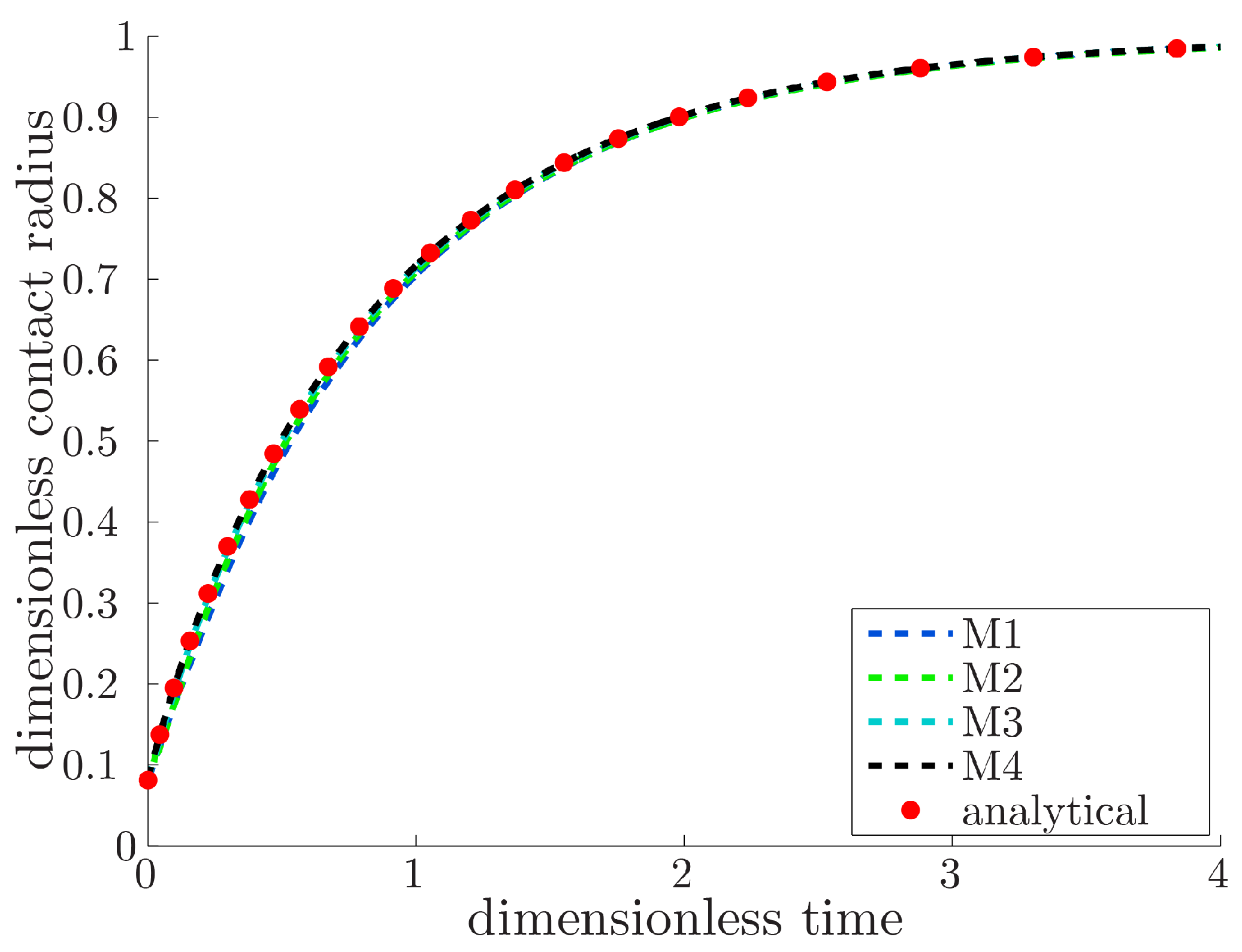
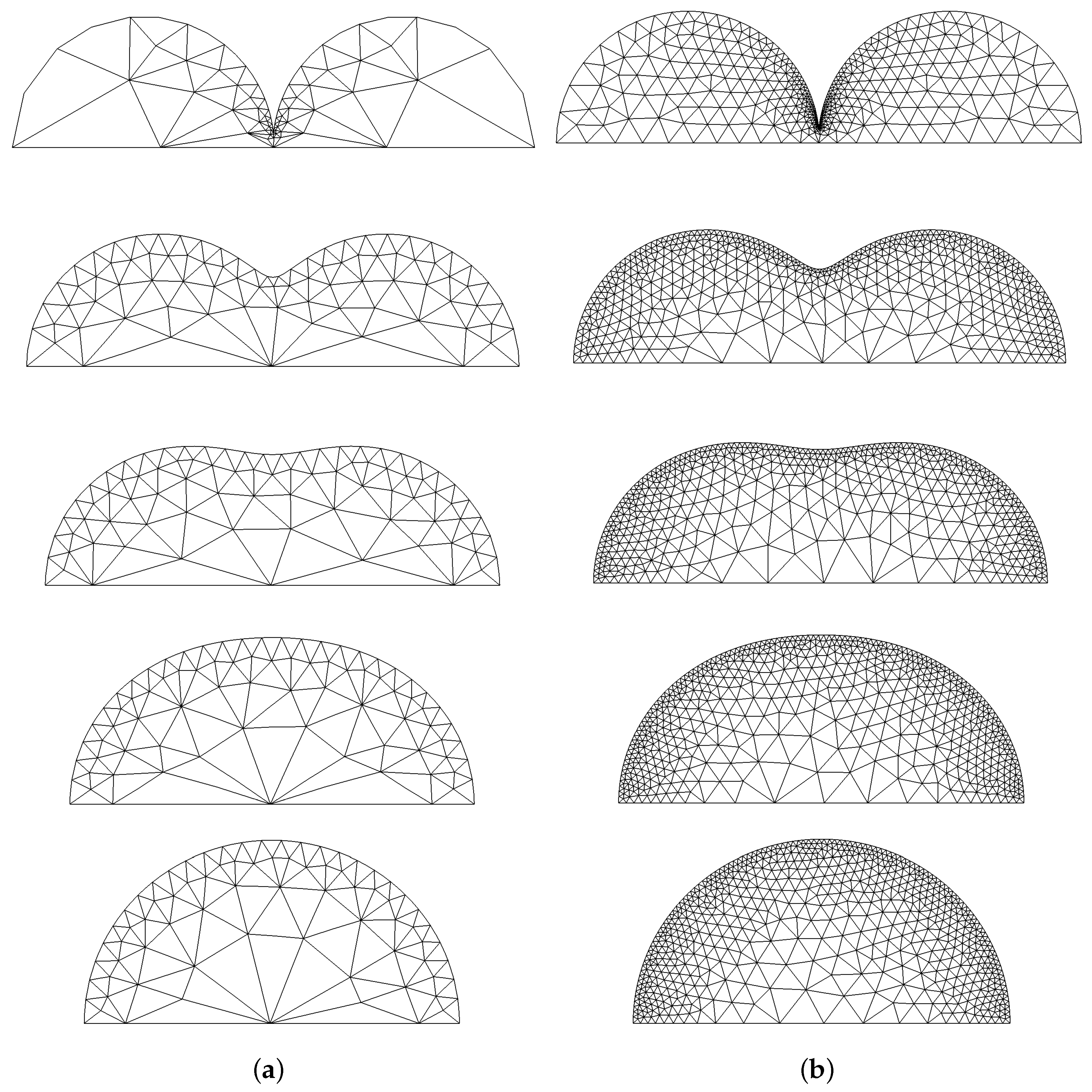
Hopper [6] derived an analytical solution for the time evolution of a creeping viscous incompressible planar flow in a finite region, bounded by a smooth closed curve and driven by surface tension only. One of the geometries gives the exact solution of the coalescence of two equal cylinders. To validate our model, we simulated the two-dimensional equivalent of the axisymmetric problem as described before with $R=1/\sqrt{2}$ and $y_{\mathrm{n}}=0.075$. We used the Newtonian constitutive equation with $\mu =1$ and $\gamma =1$ for the simulations. The results of the contact radius y in time t of the FEM calculations (meshes M1 to M4 in Table 2) are compared to Hopper’s solution and are shown in Figure 2. Note that the dimensionless time and contact radius are scaled using $R_{\mathrm{final}}=1$ instead of R and that Hopper’s dimensionless time is set to $t=0$ if the contact radius $y=0.075+w$. As a demonstration of the remeshing procedure discussed in Section 4.2, the dynamic evolution of meshes M1 and M4 is shown in Figure 3.

Table 2. Mesh resolution of different surface meshes used in the convergence study.

Mesh	${\mathit{h}}_{\mathbf{coarse}}$	${\mathit{h}}_{\mathbf{fine}}$	Number of Nodes on the Surface
M1	1.05	0.015	59
M2	0.7	0.01	67
M3	0.35	0.005	119
M4	0.175	0.0025	223

Figure 2. The evolution of the contact radius y in time t of two equal cylinders, obtained by FEM analyses with different surface meshes and by the analytical solution of Hopper [6], with the initial contact radius $y=0.075+w$ at time $t=0$.

Figure 3. Dynamic evolution of the sintering process at times $t=[0,0.5,1,2,4]$ for M1 (a) and M4 (b).

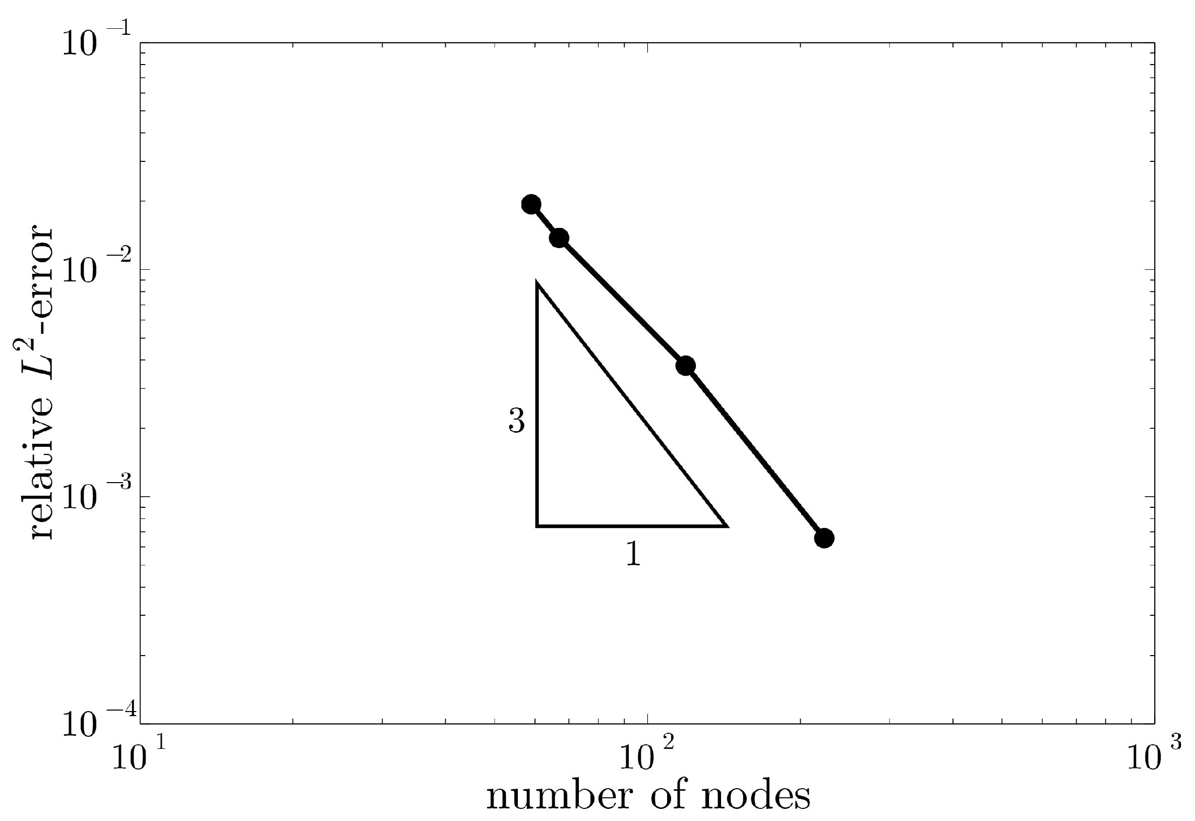
The FEM simulations are performed on four different meshes to study mesh convergence, as given in Table 2. The relative $L^2$-error of the contact radius y is determined from 23 measurements in time interval $0\le t\le 3.8375$ (red dots in Figure 2), defined as:

$${\epsilon }_y={\displaystyle \frac{{\left({\sum }_{k=1}^{23}{(y_k^h-y_k^{*})}^2\right)}^{\frac{1}{2}}}{{\left({\sum }_{k=1}^{23}{\left(y_k^{*}\right)}^2\right)}^{\frac{1}{2}}}},$$

(44)

where $y^h$ is the solution of one of the meshes given in Table 2 and $y^{*}$ is the analytical solution. The convergence plot is shown Figure 4. The convergence of the error of the contact radius is third-order, which is as expected from the second-order elements. We will continue using the h-values of the finest mesh M4 in the rest of the work.

Figure 4. Mesh convergence for the contact radius y.

6. Results

6.1. Effect of the Initial Geometry

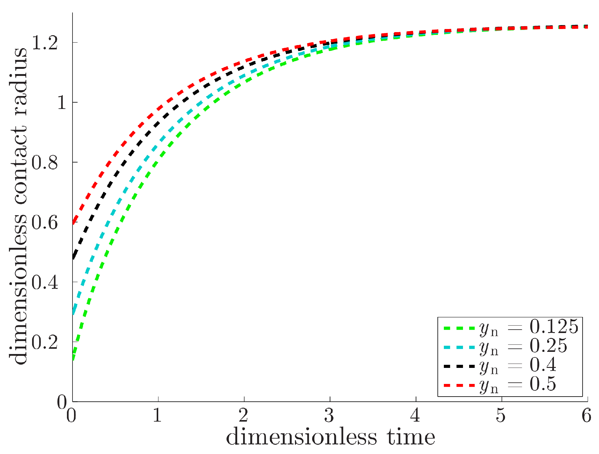
From the governing equations of the Newtonian constitutive behavior follows that the initial geometry and configuration are the only factors that affect the flow. To analyze the influence of different initial contact radii, we define four geometries: $R=1$ and $y_{\mathrm{n}}=[0.125,0.25,0.4,0.5]$. Without loss of generality, we set the viscosity $\mu =1$ and the surface tension $\gamma =1$. The results are shown in Figure 5, where the contact radius y is depicted in time t.

Figure 5. The evolution of the contact radius y in time t of two equal spheres with different initial contact radii $y_{\mathrm{n}}=[0.125,0.25,0.4,0.5]$, using the Newtonian constitutive equation.

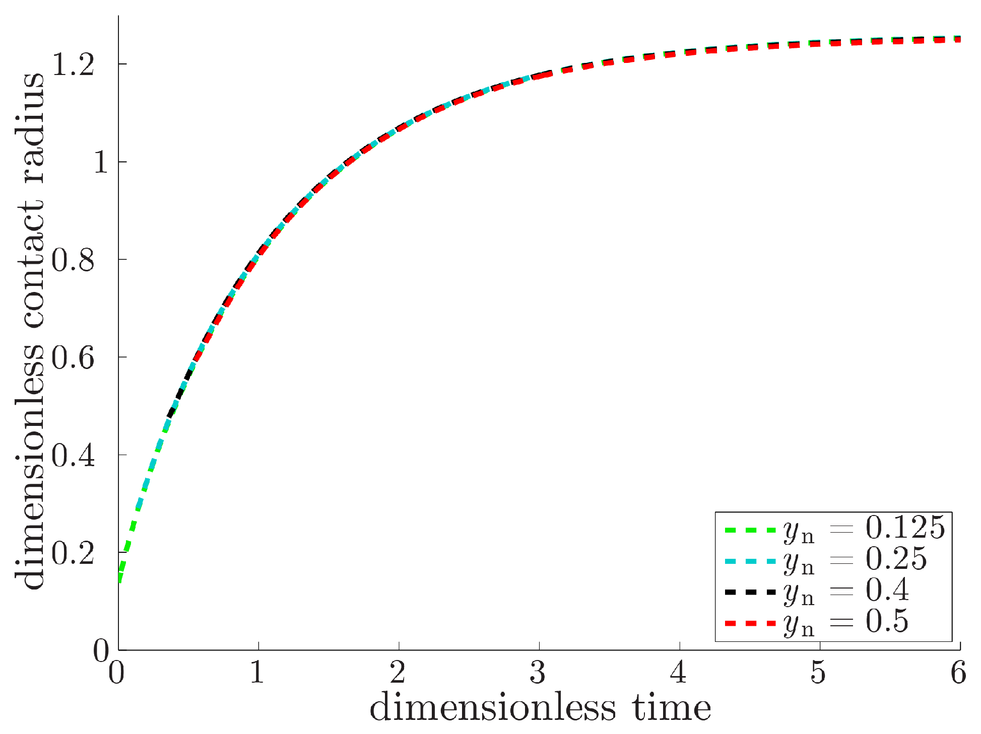
Subsequently, we shift the graphs of $y_{\mathrm{n}}=0.25$, $y_{\mathrm{n}}=0.4$ and $y_{\mathrm{n}}=0.5$ in time such that the initial contact radii coincide with the curve of $y_{\mathrm{n}}=0.125$. The results are given in Figure 6, in which we see that all lines overlap. This indicates that the shape evolution of the contact radius y is independent of the flow history, if the round off parameter $R_{\mathrm{n}}=R\times {(y_{\mathrm{n}}/R)}^3$ [20] is used.

Figure 6. The evolution of the contact radius y in time t of two equal spheres with different initial contact radii $y_{\mathrm{n}}=[0.125,0.25,0.4,0.5]$, using the Newtonian constitutive equation. The lines of $y_{\mathrm{n}}=0.25$, $y_{\mathrm{n}}=0.4$ and $y_{\mathrm{n}}=0.5$ are shifted in time such that the initial contact radii coincide with the graph of $y_{\mathrm{n}}=0.125$.

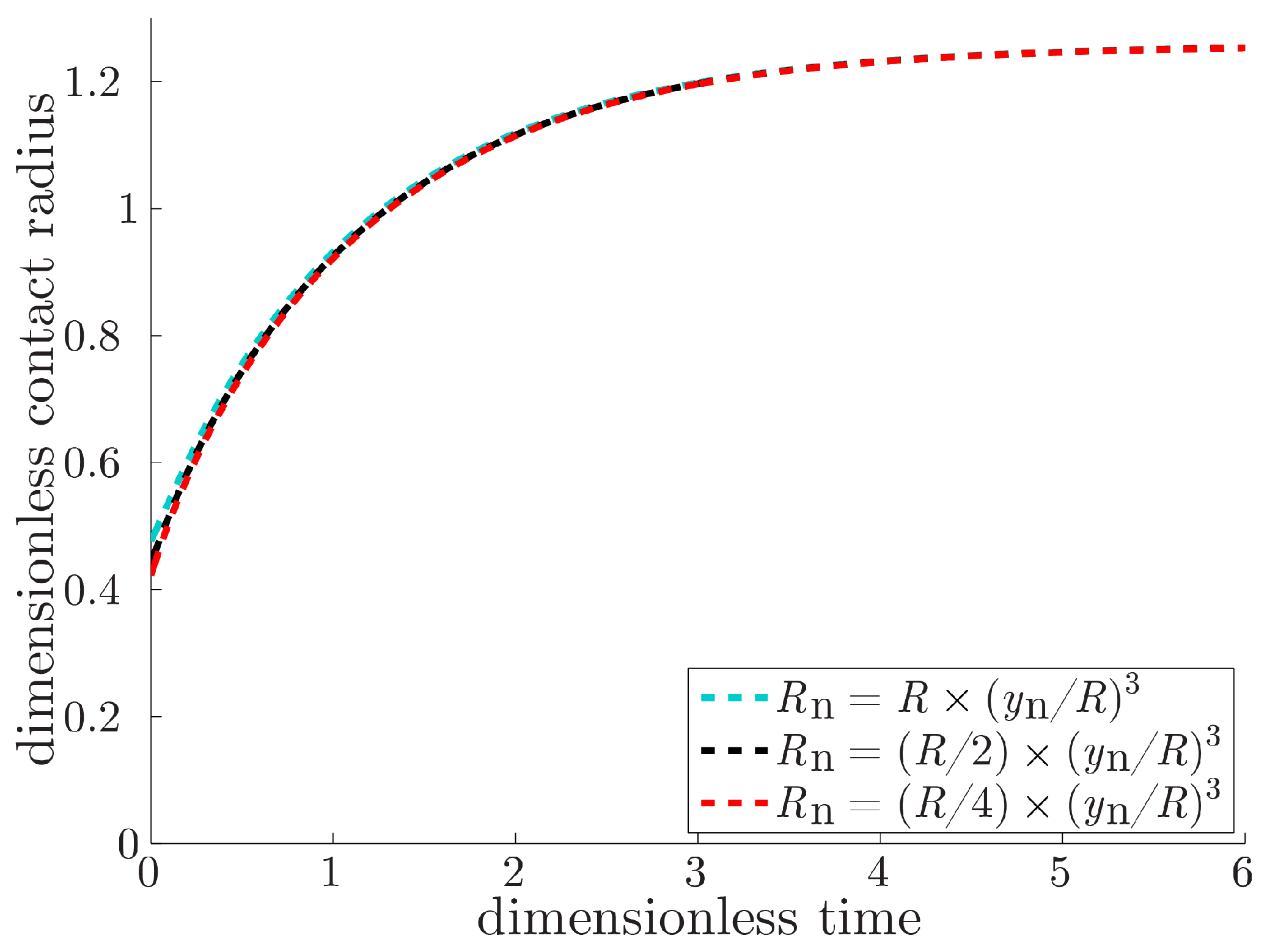
Next, we keep the initial contact radius constant $y_{\mathrm{n}}=0.4$, and we change the round off parameter $R_{\mathrm{n}}=[R\times {(y_{\mathrm{n}}/R)}^3,(R/2)\times {(y_{\mathrm{n}}/R)}^3,(R/4)\times {(y_{\mathrm{n}}/R)}^3]$. The results are given in Figure 7, where the contact radius y is depicted in time t. Since all curves coincide, we can conclude that the influence of the round off parameter $R_{\mathrm{n}}$ on the shape evolution of the contact radius y is negligible.

Figure 7. The evolution of the contact radius y in time t of two equal spheres with initial contact radius $y_{\mathrm{n}}=0.4$ and different round off parameters $R_{\mathrm{n}}=[R\times {(y_{\mathrm{n}}/R)}^3,(R/2)\times {(y_{\mathrm{n}}/R)}^3,(R/4)\times {(y_{\mathrm{n}}/R)}^3]$, using the Newtonian constitutive equation.

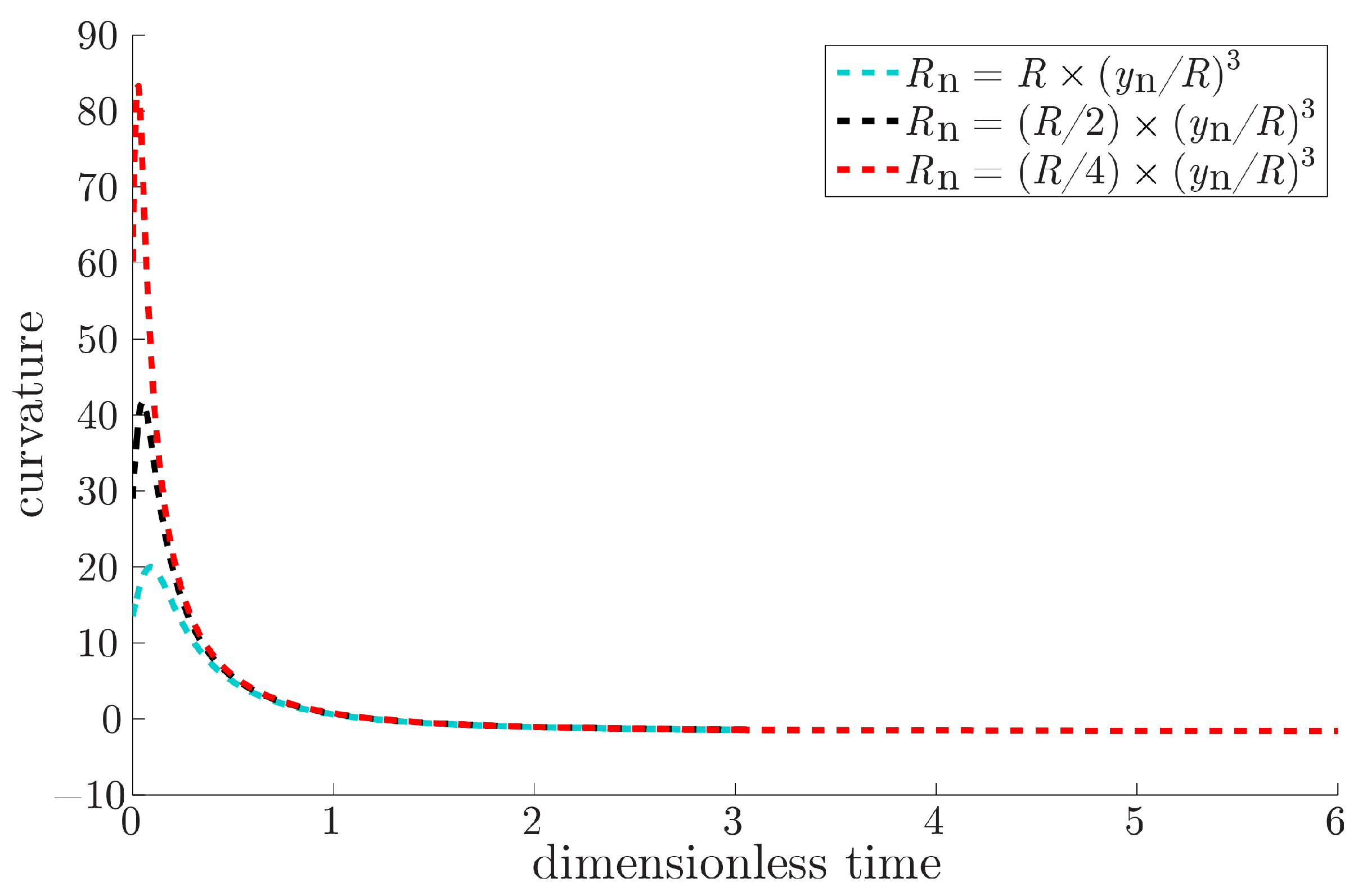
Furthermore, the curvature $\kappa$ at point $(0,y)$ at the surface of the neck is shown in time t for different round off parameters $R_{\mathrm{n}}=[R\times {(y_{\mathrm{n}}/R)}^3,(R/2)\times {(y_{\mathrm{n}}/R)}^3,(R/4)\times {(y_{\mathrm{n}}/R)}^3]$ in Figure 8. Following Dantzig and Tucker [37], the curvature is calculated from the contour curve $r=g\left(z\right)$ of surface $\mathrm{\Gamma }$, using:

$$\kappa ={\displaystyle \frac{1}{R_1}}+{\displaystyle \frac{1}{R_2}},$$

(45)

with $R_1$ and $R_2$ the two principal radii of curvature:

$$\begin{array}{c}\hfill R_1={\displaystyle \frac{{(1+g^{\prime 2})}^{3/2}}{g^{″}}},\end{array}$$

(46)

$$\begin{array}{c}\hfill R_2=-g\sqrt{1+g^{\prime 2}}.\end{array}$$

(47)

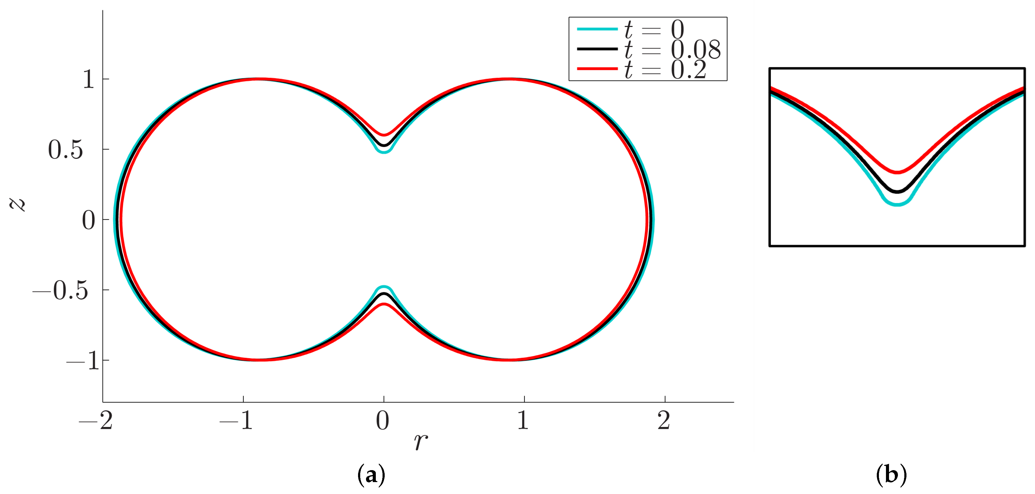
Herein, $g^{\prime }=dg/dz$ and $g^{″}=d^{2}g/d{z}^2$. From the curvature, the Laplace pressure $p_{\mathrm{L}}$ can be calculated using $p_{\mathrm{L}}=\gamma \kappa$, which is equal to the radial component of the Cauchy stress tensor ${\sigma }_{rr}$ at the surface. From Figure 8, it follows that the curvature $\kappa$ at point $(0,y)$ increases with respect to the initial geometry until it reaches a maximum value and subsequently decreases. This holds for all different values of the round off parameter $R_{\mathrm{n}}=[R\times {(y_{\mathrm{n}}/R)}^3,(R/2)\times {(y_{\mathrm{n}}/R)}^3,(R/4)\times {(y_{\mathrm{n}}/R)}^3]$. This behavior is depicted in Figure 9, where the contour line $r=g\left(z\right)$ of the two particles is shown at times $t=[0,0.08,0.2]$, using $R_n=R\times {(y_{\mathrm{n}}/R)}^3$. Herein, $t=0.08$ is the time at which the curvature $\kappa$ reaches its maximum value. From this, we can conclude that the choice of the round off parameter $R_{\mathrm{n}}$ strongly influences the evolution of curvature and, therefore, the evolution of the local stresses in the material.

Figure 8. The evolution of the curvature $\kappa$ in time t of two equal spheres with initial contact radius $y_{\mathrm{n}}=0.4$ and different round off parameter $R_{\mathrm{n}}=[R\times {(y_{\mathrm{n}}/R)}^3,(R/2)\times {(y_{\mathrm{n}}/R)}^3,(R/4)\times {(y_{\mathrm{n}}/R)}^3]$, using the Newtonian constitutive equation.

Figure 9. The contour plot of $r=g\left(z\right)$ at time $t=[0,0.08,0.2]$ with initial contact radius $y_{\mathrm{n}}=0.4$ and round off parameter $R_{\mathrm{n}}=R\times {(y_{\mathrm{n}}/R)}^3$, using the Newtonian constitutive equation (a), and a zoom of the neck region (b).

6.2. Effect of the Rheology

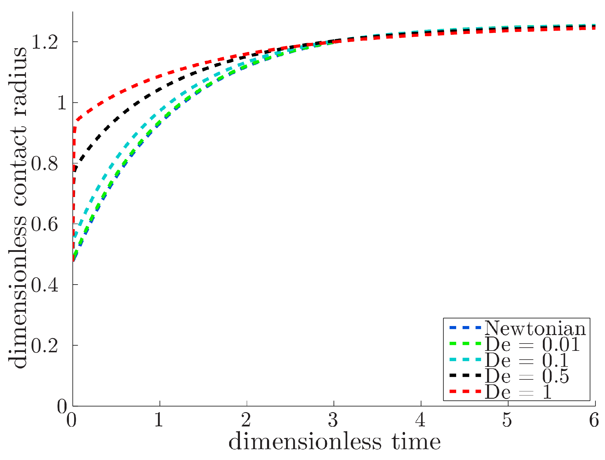
Keeping the initial geometry constant, we assess the effect of the rheological model on the flow behavior of the system. We use a geometry of two equal particles $R=1$ with initial contact radius $y_{\mathrm{n}}=0.4$ and round off parameter $R_{\mathrm{n}}=R\times {(y_{\mathrm{n}}/R)}^3$. We set the zero-shear-rate viscosity ${\eta }_0=1$, solvent viscosity ${\eta }_{\mathrm{s}}=0.01$ and surface tension $\gamma =1$. First, the Deborah number is changed by varying the relaxation time $\lambda =[0.01,0.1,0.5,1]$, resulting in Deborah numbers $\mathrm{De}=[0.01,0.1,0.5,1]$, respectively. The results are shown in Figure 10, where the contact radius y is depicted in time t, using the Giesekus constitutive model with $\alpha =0.1$.

Figure 10. The evolution of the contact radius y in time t for different Deborah numbers $\mathrm{De}=[0.01,0.1,0.5,1]$, using the Giesekus model with $\alpha =0.1$. The result of the Newtonian behavior is included, as well.

With increasing Deborah number, the initial increase in contact radius between $t=0$ and $t=0.05$ gets larger. By keeping the viscosity constant and varying the relaxation time, the modulus is changed $G={\eta }_{\mathrm{p}}/\lambda =[100,10,2,1]$, respectively. Initially, $\stackrel{▿}{\mathit{c}}=0$, and from this, it follows that $\mathit{c}=\mathit{B}$ and $\mathit{\tau }=G(\mathit{B}-\mathit{I}),$ where $\mathit{B}$ is the Finger tensor. Since $\mathit{\tau }$ scales with $\gamma /R$, which is kept constant, the Finger tensor $\mathit{B}$ has to increase for decreasing modulus G. Consequently, the initial deformation increases for increasing Deborah number as shown in Figure 10. The deformation is not completely instantaneous, because ${\eta }_{\mathrm{s}}>0$. From $t=0.05$ onwards, the shape transition gets slower for increasing Deborah number. From simulations, it follows that the same behavior holds for the XPP constitutive model.

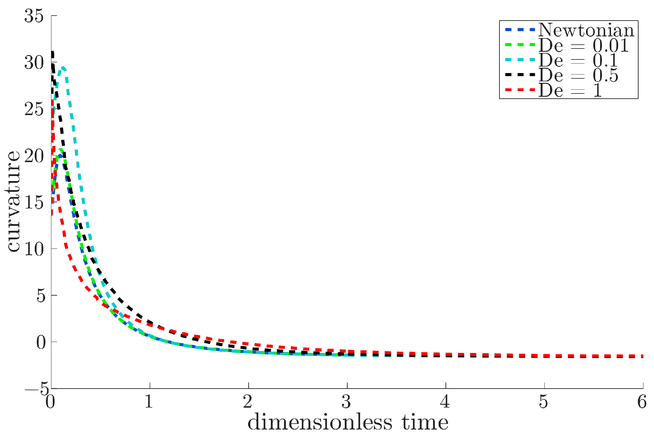
In Figure 11, the curvature $\kappa$ at point $(0,y)$ at the surface of the neck is shown in time t for different Deborah numbers $\mathrm{De}=[0.01,0.1,0.5,1]$, using the Giesekus model with $\alpha =0.1$. As is shown for the Newtonian constitutive behavior, the curvature $\kappa$ at point $(0,y)$ increases with respect to the initial geometry until it reaches a maximum value and subsequently decreases for all different values of the Deborah number $\mathrm{De}=[0.01,0.1,0.5,1]$, as well. The maximum value of the curvature $\kappa$ and the time t of the maximum depend on the value of the Deborah number De.

Figure 11. The curvature $\kappa$ at point $(0,y)$ at the surface of the neck in time t for different Deborah numbers $\mathrm{De}=[0.01,0.1,0.5,1]$, using the Giesekus model with $\alpha =0.1$. The result of the Newtonian behavior is included, as well.

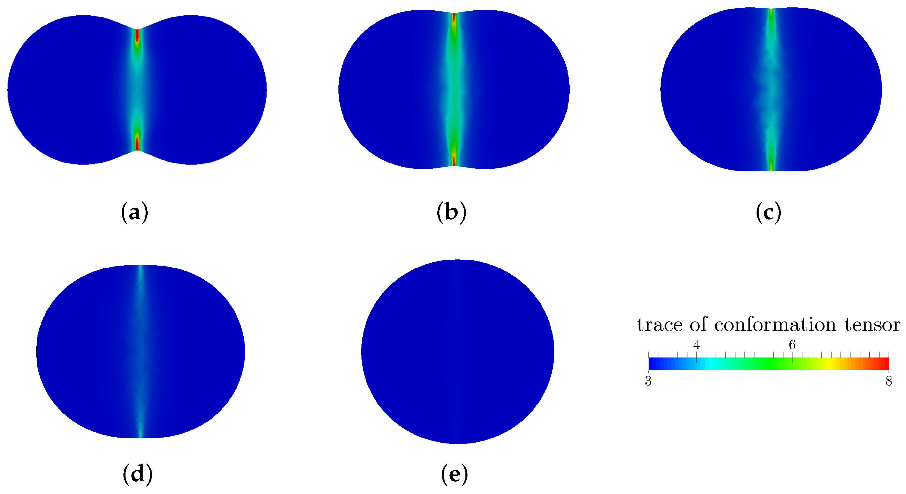
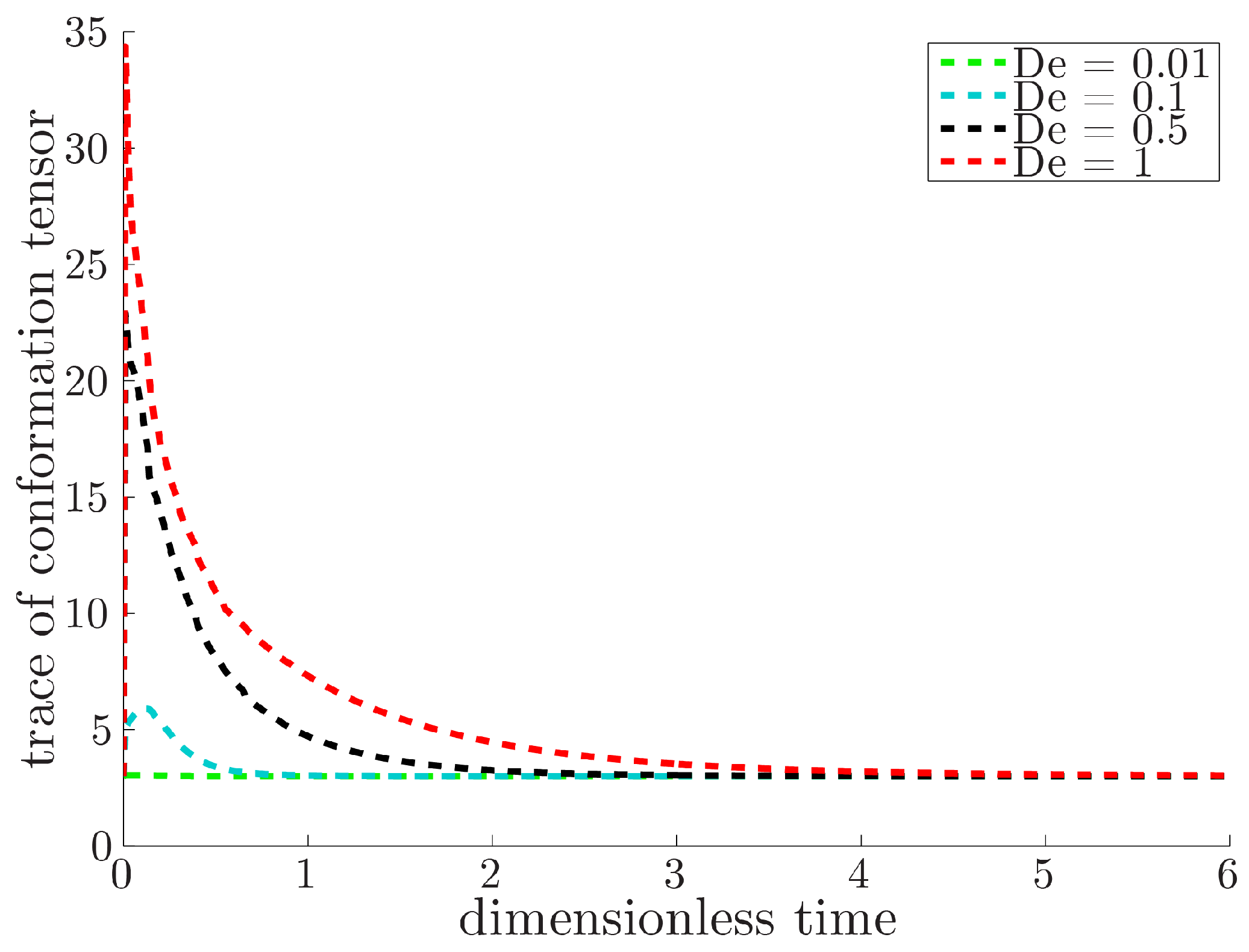
Furthermore, we assess the conformation tensor $\mathit{c}$, which is a measure for the polymeric strain in the system and plays an important role in the crystallization kinetics of semicrystalline polymers like PA12. The dynamic evolution of the trace of the conformation tensor $\mathrm{tr}\left(\mathit{c}\right)$, using the Giesekus constitutive model with $\alpha =0.1$ and $\mathrm{De}=1$, is shown in Figure 12. For visualization, the color bar ranges from three to eight, but the values locally exceed these numbers.

Figure 12. Dynamic evolution of the trace of the conformation tensor $\mathrm{tr}\left(\mathit{c}\right)$ at $t=[0.01,0.5,1,2,5]$, using the Giesekus model with $\alpha =0.1$ and $\mathrm{De}=1$; note that the real values locally exceed the values shown in the color bar (see Figure 13).

From Figure 12, it can be seen that elevated polymeric strains are present throughout the contact area between the two particles. This might lead to crystalline structures in large parts of the system and influences the material characteristics of sintered products. The trace of the conformation tensor $\mathrm{tr}\left(\mathit{c}\right)$ at point $(0,y)$ at the surface of the neck in time t for different Deborah numbers $\mathrm{De}=[0.01,0.1,0.5,1]$, using the Giesekus model with $\alpha =0.1$, is shown in Figure 13. The polymeric strain increases with increasing Deborah number and is negligibly small for $\mathrm{De}=0.01$.

Figure 13. The trace of the conformation tensor $\mathrm{tr}\left(\mathit{c}\right)$ at point $(0,y)$ at the surface of the neck in time t for different Deborah numbers $\mathrm{De}=[0.01,0.1,0.5,1]$, using the Giesekus model with $\alpha =0.1$.

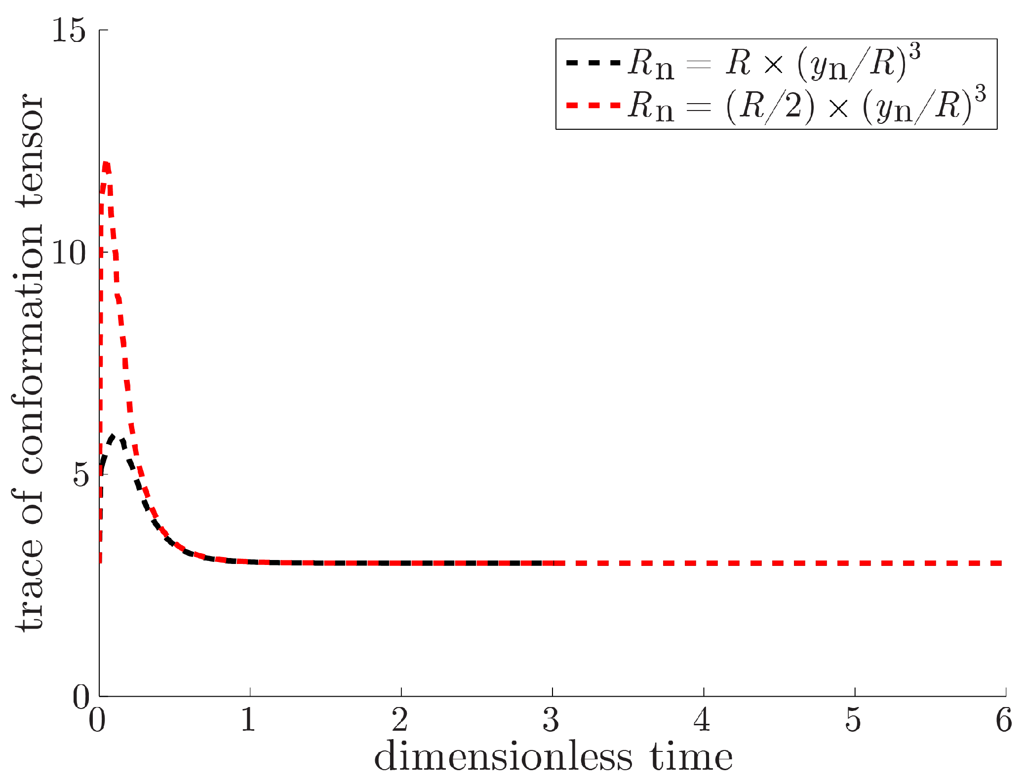
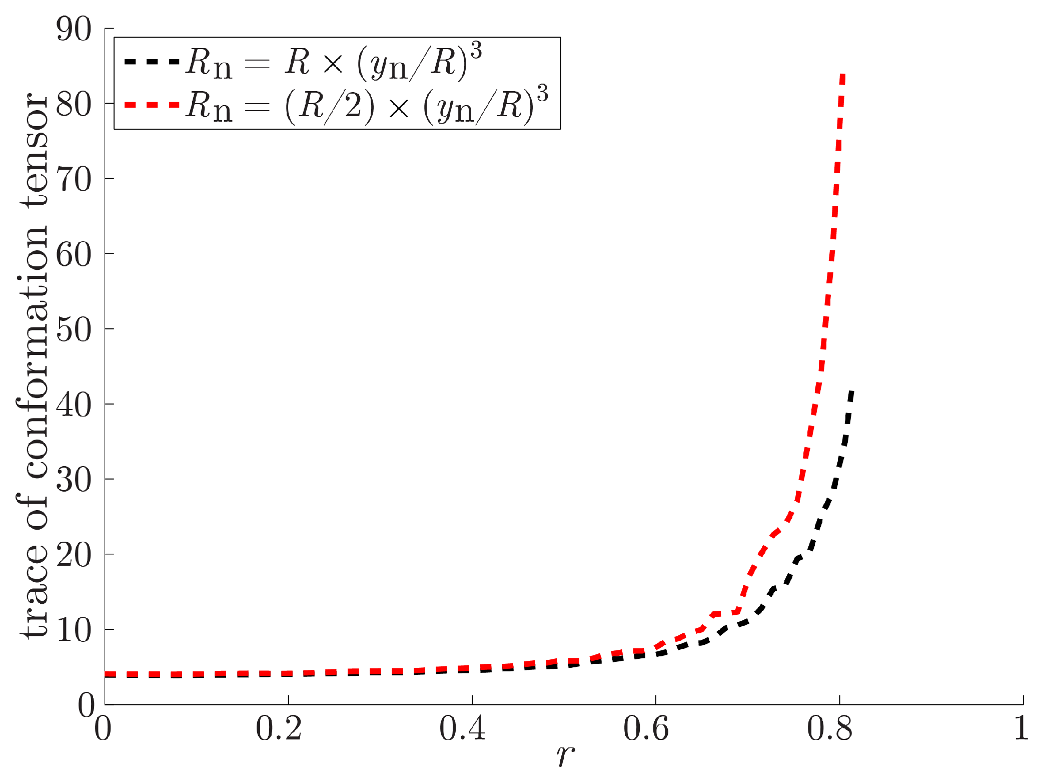
Furthermore, decreasing the round off parameter $R_{\mathrm{n}}$ leads to an increase in the polymeric strain, as shown in Figure 14 for different $R_{\mathrm{n}}=[R\times {(y_{\mathrm{n}}/R)}^3,(R/2)\times {(y_{\mathrm{n}}/R)}^3]$, using the Giesekus model with $\alpha =0.1$ and $\mathrm{De}=0.1$. Looking at a cross-section of the contact area between the two particles, as shown in Figure 15, where the trace of the conformation tensor $\mathrm{tr}\left(\mathit{c}\right)$ is given versus the coordinate of the contact area $(0,r)$ at time $t=0.01$ for different $R_{\mathrm{n}}=[R\times {(y_{\mathrm{n}}/R)}^3,(R/2)\times {(y_{\mathrm{n}}/R)}^3]$, using the Giesekus model with $\alpha =0.1$ and $\mathrm{De}=1$, we can conclude that the increase in polymeric strain is not just a local effect. The fluctuations in the trace of the conformation tensor $\mathrm{tr}\left(\mathit{c}\right)$ disappear if a finer mesh is used. Although we possibly underestimate the polymeric strain in the system, we continue using the round off parameter $R_{\mathrm{n}}=R\times {(y_{\mathrm{n}}/R)}^3$ in the remaining part of this work.

Figure 14. The trace of the conformation tensor $\mathrm{tr}\left(\mathit{c}\right)$ at point $(0,y)$ at the surface of the neck in time t for different round off parameters $R_{\mathrm{n}}=[R\times {(y_{\mathrm{n}}/R)}^3,(R/2)\times {(y_{\mathrm{n}}/R)}^3]$, using the Giesekus model with $\alpha =0.1$ and $\mathrm{De}=0.1$.

Figure 15. The trace of the conformation tensor $\mathrm{tr}\left(\mathit{c}\right)$ versus the coordinate of the contact area $(0,r)$ at time $t=0.01$ for different $R_{\mathrm{n}}=[R\times {(y_{\mathrm{n}}/R)}^3,(R/2)\times {(y_{\mathrm{n}}/R)}^3]$, using the Giesekus model with $\alpha =0.1$ and $\mathrm{De}=1$.

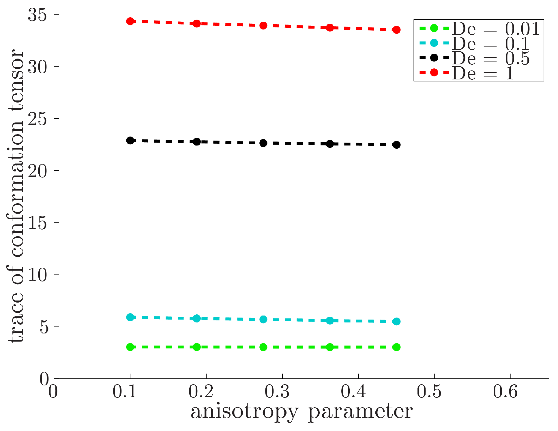
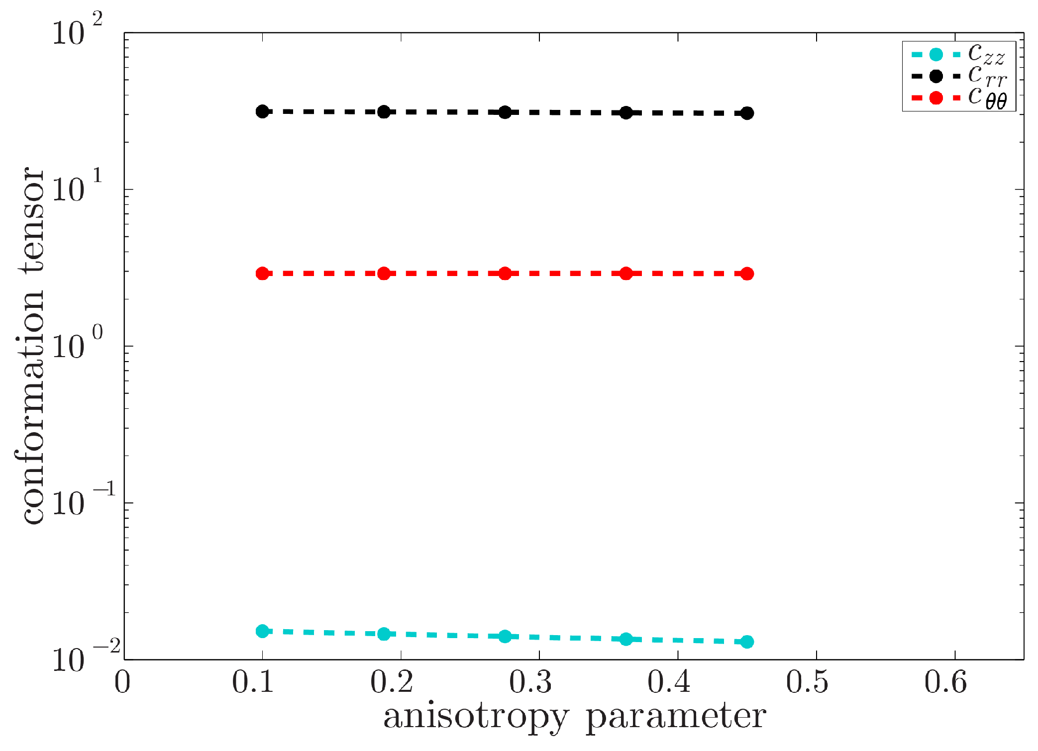
In the Giesekus constitutive model, the anisotropy parameter $\alpha$ is, besides the Deborah number De, another dimensionless parameter that determines the flow behavior of the system. The maximum values of the trace of the conformation tensor $\mathrm{tr}\left(\mathit{c}\right)$ for different Deborah numbers $\mathrm{De}=[0.01,0.1,0.5,1]$ and anisotropy parameter $\alpha =[0.1,0.1875,0.275,0.3625,0.45]$ are shown in Figure 16. The maximum values of the trace of the conformation tensor $\mathrm{tr}\left(\mathit{c}\right)$ occur during the start-up of the flow, which is primarily driven by elastic effects. The elastic stresses are determined by the modulus G and the strain. The anisotropy parameter $\alpha$ determines the non-linear relaxation, and therefore, $\alpha$ has only a small influence on the stresses during the start-up of the flow.

Figure 16. The maximum value of the trace of the conformation tensor $\mathrm{tr}\left(\mathit{c}\right)$ for different Deborah numbers $\mathrm{De}=[0.01,0.1,0.5,1]$ and anisotropy parameter $\alpha =[0.1,0.1875,0.275,0.3625,0.45]$, using the Giesekus model.

In Figure 17, the three entries of the trace of the conformation tensor $c_{zz}$, $c_{rr}$ and $c_{\theta \theta }$ are shown separately for the highest value of the trace, using the Giesekus model with $\mathrm{De}=1$ and $\alpha =[0.1,0.1875,0.275,0.3625,0.45]$. The value of $c_{zz}$ is smaller than one, which means that the polymer chains are compressed in the axial direction. Furthermore, $c_{rr}$ is the highest value, which means that the polymer chains are stretched the most in the radial direction. The value of $c_{\theta \theta }$ is in the order of four, which is expected from the value of the tangential component of the Finger tensor $B_{\theta \theta }={(y_{t=0.05}/y_{t=0})}^2\approx 4$ at point $(0,y)$ at the surface of the neck.

Figure 17. The three entries of the trace of the conformation tensor $c_{zz}$, $c_{rr}$ and $c_{\theta \theta }$ for the maximum value of the trace for different $\alpha =[0.1,0.1875,0.275,0.3625,0.45]$, using the Giesekus model with $\mathrm{De}=1$.

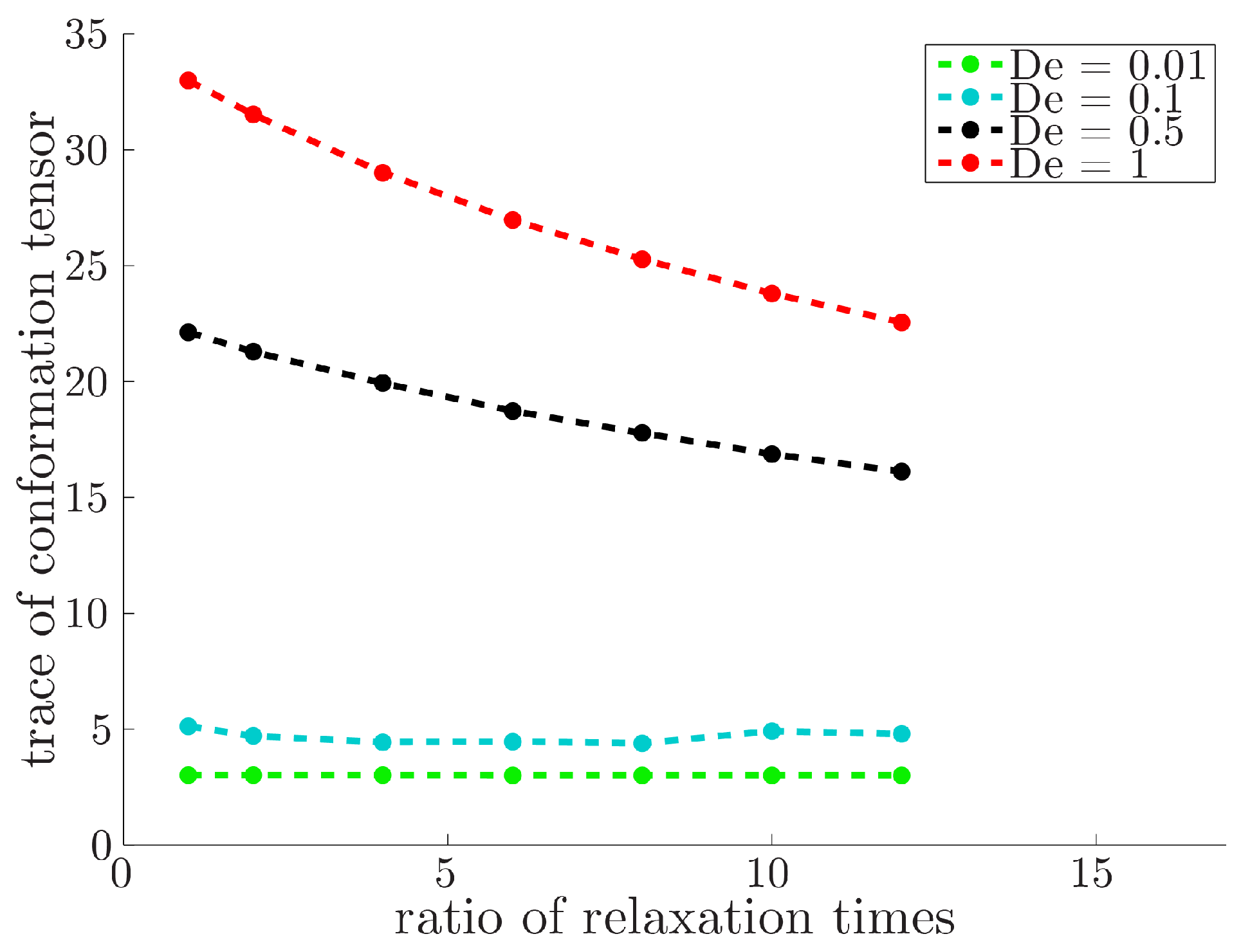
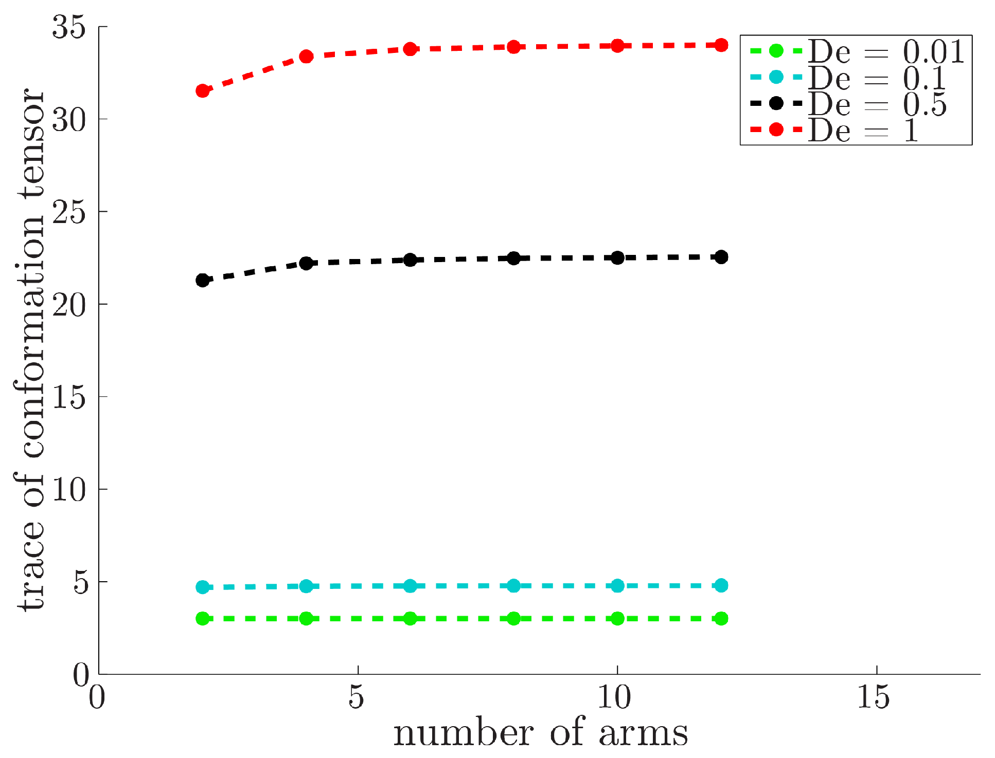
In the XPP constitutive model, both the ratio between the relaxation time of the backbone orientation and that of the stretch $\xi$ and the number of arms q are dimensionless parameters defining the rheological behavior of the system, apart from the Deborah number De. In Figure 18 and Figure 19, the maximum values of the trace of the conformation tensor $\mathrm{tr}\left(\mathit{c}\right)$ for different Deborah numbers $\mathrm{De}=[0.01,0.1,0.5,1]$ are shown for $\xi =[1,2,4,6,8,10,12]$, with $q=2$, and $q=[2,4,6,8,10,12]$, with $\xi =2$, respectively. Both the relaxation time ratio $\xi$ and the number of arms q influence only the results with the highest Deborah numbers $\mathrm{De}=[0.5,1]$. With increasing ratio $\xi$, the relaxation time of the stretch ${\lambda }_{\mathrm{s}}$ decreases with respect to the relaxation time of the backbone orientation $\lambda$. Therefore, the polymers are harder to stretch, and the maximum value of the trace of the conformation tensor $\mathrm{tr}\left(\mathit{c}\right)$ decreases. Increasing the number of arms q leads to an increase in the relaxation time of the stretch ${\lambda }_{\mathrm{s}}$. Since the polymer chains are easier to stretch, the maximum value of the trace of the conformation tensor $\mathrm{tr}\left(\mathit{c}\right)$ increases with increasing number of arms q. This effect is visible only for the number of arms $q<6$.

Figure 18. The maximum value of the trace of the conformation tensor for different Deborah numbers $\mathrm{De}=[0.01,0.1,0.5,1]$ and the ratio between the relaxation time of the backbone orientation and that of the stretch $\xi =[1,2,4,6,8,10,12]$, using the XPP model with $q=2$.

Figure 19. The maximum value of the trace of the conformation tensor for different Deborah number $\mathrm{De}=[0.01,0.1,0.5,1]$ and the number of arms $q=[2,4,6,8,10,12]$, using the XPP model with $\xi =2$.

7. Conclusions

We developed a numerical model to study the basics of the sintering process of polymer powder for additive manufacturing (SLS). The isothermal flow is solved using the finite element method for fluids following Newtonian, Giesekus and XPP constitutive behavior on an axisymmetric geometry of two spherical particles, initially connected by a neck with a certain radius.

The computational model has been validated with the analytical solution as described by Hopper [6], which gives the time evolution of a creeping viscous incompressible planar flow of a finite region, bounded by a smooth closed surface and driven by surface tension. Furthermore, convergence towards the analytical solution is shown for different surface mesh sizes, where the mesh with the smallest elements gives the best match and is used for all of the following simulations.

For Newtonian fluids, the shape transition depends only on the initial geometry, as can be concluded from the dimensionless description of the problem. From simulations where the radii of the spheres are kept constant and the initial neck radius is changed, we can conclude that the shape evolution of the contact radius is independent of the flow history if the round off parameter $R_{\mathrm{n}}=R\times {(y_{\mathrm{n}}/R)}^3$ [20] is used. Changing the round off parameter has no visible effect on the shape evolution of the contact radius, but strongly influences the evolution of the curvature of the surface and local stresses in the system.

Furthermore, we assessed the effect of different dimensionless numbers in both the Giesekus and XPP constitutive model on the shape and conformation tensor. With respect to the shape transition of the system, we found that increasing the Deborah number, i.e., increasing the relaxation time while keeping the viscosity unchanged, leads to a decrease in modulus and subsequently to an increase in initial deformation. Furthermore, the curvature of the surface in the neck region, where the two particles are connected, increases in time until it reaches a maximum value, after which it decreases. This behavior is shown for all different values of the Deborah number, as well as for the Newtonian constitutive model. The conformation tensor, which is a measure for the polymeric strain, plays an important role in the crystallization kinetics of semicrystalline polymers. The dynamic evolution of the trace of the conformation tensor showed that elevated polymeric strains are present throughout the contact area between the two particles, influencing the material characteristics of sintered products. Decreasing the round off parameter $R_{\mathrm{n}}$ leads to an increase of polymeric strain. The anisotropy parameter in the Giesekus model shows a negligible effect on the maximum value of the trace of the conformation tensor. The relaxation time ratio and the number of arms in the XPP model influence only the results with higher values of the Deborah number. Decreasing the relaxation time ratio and increasing the number of arms both increase the relaxation time of the stretch, leading to a higher maximum value of the polymeric strain. Note that we possibly underestimated the polymeric strain in the system, since we used the round off parameter $R_{\mathrm{n}}=R\times {(y_{\mathrm{n}}/R)}^3$ [20].

References

- Frenkel, J. Viscous flow of crystalline bodies under the action of surface tension. J. Phys. IX 1945, 5, 385–391. [Google Scholar]
- Eshelby, J. Discussion of ‘Seminar on the kinetics of sintering’. Metall. Trans. 1949, 185, 796–813. [Google Scholar]
- Pokluda, O.; Bellehumeur, C.; Vlachopoulos, J. Modification of Frenkel’s model for sintering. AIChE J. 1997, 43, 3253–3256. [Google Scholar] [CrossRef]
- Bellehumeur, C.; Kontopoulou, M.; Vlachopoulos, J. The role of viscoelasticity in polymer sintering. Rheol. Acta 1998, 37, 270–278. [Google Scholar] [CrossRef]
- Scribben, E.; Baird, D.; Wapperom, P. The role of transient rheology in polymeric sintering. Rheol. Acta 2006, 45, 825–839. [Google Scholar] [CrossRef]
- Hopper, R. Plane Stokes flow driven by capillarity on a free surface. J. Fluid Mech. 1990, 213, 349–375. [Google Scholar] [CrossRef]
- Richardson, S. Two-dimensional slow viscous flows with time-dependent free boundaries driven by surface tension. Eur. J. Appl. Math. 1992, 3, 193–207. [Google Scholar] [CrossRef]
- Crowdy, D. Exact solutions for the viscous sintering of multiply-connected fluid domains. J. Eng. Math. 2002, 42, 225–242. [Google Scholar] [CrossRef]
- Bellehumeur, C.; Bisaria, M.; Vlachopoulos, J. An experimental study and model assessment of polymer sintering. Polym. Eng. Sci. 1996, 36, 2198–2207. [Google Scholar] [CrossRef]
- Mazur, S.; Plazek, D. Viscoelastic effects in the coalescence of polymer particles. Prog. Org. Coat. 1994, 24, 225–236. [Google Scholar] [CrossRef]
- Ross, J.; Miller, W.; Weatherly, C. Dynamic computer simulation of viscous flow sintering kinetics. J. Appl. Phys. 1981, 52, 3884–3888. [Google Scholar] [CrossRef]
- Kuiken, H. Viscous sintering: the surface-tension-driven flow of a liquid form under the influence of curvature gradients at its surface. J. Fluid Mech. 1990, 214, 503–515. [Google Scholar] [CrossRef]
- Van de Vorst, G. Integral method for a two-dimensional Stokes flow with shrinking holes applied to viscous sintering. J. Fluid Mech. 1993, 257, 667–689. [Google Scholar] [CrossRef]
- Martínez-Herrera, J.; Derby, J. Analysis of capillary-driven viscous flows during the sintering of ceramic powders. AIChE J. 1994, 40, 1794–1803. [Google Scholar] [CrossRef]
- Jagota, A.; Dawson, P. Micromechanical modeling of powder compacts-I: Unit problems for sintering and traction induced deformation. Acta Metall. 1988, 36, 2551–2561. [Google Scholar] [CrossRef]
- Jagota, A.; Dawson, P. Simulation of the viscous sintering of two particles. J. Am. Ceram. Soc. 1990, 73, 173–177. [Google Scholar] [CrossRef]
- Van de Vorst, G. Numerical simulation of axisymmetric viscous sintering. Eng. Anal. Bound. Elem. 1994, 14, 193–207. [Google Scholar] [CrossRef]
- Martínez-Herrera, J.; Derby, J. Viscous sintering of spherical particles via finite element analysis. J. Am. Ceram. Soc. 1995, 78, 645–649. [Google Scholar] [CrossRef]
- Zhou, H.; Derby, J. Three-dimensional finite element analysis of viscous sintering. J. Am. Ceram. Soc. 1998, 81, 533–540. [Google Scholar] [CrossRef]
- Hooper, R.; Macosko, C.; Derby, J. Assessing a flow-based finite element model for the sintering of viscoelastic particles. Chem. Eng. Sci. 2000, 55, 5733–5746. [Google Scholar] [CrossRef]
- Verbeeten, W.; Peters, G.; Baaijens, F. Differential constitutive equations for polymer melts: The extended Pom-Pom model. J. Rheol. 2001, 45, 823–843. [Google Scholar] [CrossRef]
- Balemans, C.; Hulsen, M.; Anderson, P. Modeling of complex interfaces for pendant drop experiments. Rheol. Acta 2016, 55, 801–822. [Google Scholar] [CrossRef]
- Ellis, B.; Smith, R. Polymers: A Property Database; CRC Press: Boca Raton, FL, USA, 2008; ISBN 9780849339400. [Google Scholar]
- Wudy, K.; Drummer, D.; Drexler, M. Characterization of polymer materials and powders for selective laser melting. AIP Conf. Proc. 2014, 1593, 702–707. [Google Scholar] [CrossRef]
- Haworth, B.; Hopkinson, N.; Hitt, D.; Zhong, X. Shear viscosity measurements on Polyamide-12 polymers for laser sintering. Rapid Prototyp. J. 2013, 19, 28–36. [Google Scholar] [CrossRef]
- Villone, M.; Hulsen, M.; Anderson, P.; Maffettone, P. Simulations of deformable systems in fluids under shear flow using an arbitrary Lagrangian Eulerian technique. Comput. Fluids 2014, 90, 88–100. [Google Scholar] [CrossRef]
- Weatherburn, C. Differential Geometry of Three Dimensions; Cambridge University Press: Cambridge, UK, 1955; ISBN 9781316603840. [Google Scholar]
- Guénette, R.; Fortin, M. A new mixed finite element method for computing viscoelastic flows. J. Non-Newton. Fluid Mech. 1995, 60, 27–52. [Google Scholar] [CrossRef]
- Baaijens, F. Mixed finite element methods for viscoelastic flow analysis: A review. J. Non-Newton. Fluid Mech. 1998, 79, 361–385. [Google Scholar] [CrossRef]
- Bogaerds, A.; Grillet, A.; Peters, G.; Baaijens, F. Stability analysis of polymer shear flows using the extended Pom-Pom constitutive equations. J. Non-Newton. Fluid Mech. 2002, 108, 187–208. [Google Scholar] [CrossRef]
- Brooks, A.; Hughes, T. Streamline upwind/Petrov-Galerkin formulations for convection dominated flows with particular emphasis on the incompressible Navier-Stokes equations. Comput. Methods Appl. Mech. Eng. 1982, 32, 199–259. [Google Scholar] [CrossRef]
- Fattal, R.; Kupferman, R. Constitutive laws for the matrix-logarithm of the conformation tensor. J. Non-Newton. Fluid Mech. 2004, 123, 281–285. [Google Scholar] [CrossRef]
- Hulsen, M.; Fattal, R.; Kupferman, R. Flow of viscoelastic fluids past a cylinder at high Weissenberg number: Stabilized simulations using matrix logarithms. J. Non-Newton. Fluid Mech. 2005, 127, 27–39. [Google Scholar] [CrossRef]
- D’Avino, G.; Hulsen, M. Decoupled second-order transient schemes for the flow of viscoelastic fluids without a viscous solvent contribution. J. Non-Newton. Fluid Mech. 2010, 165, 1602–1612. [Google Scholar] [CrossRef]
- Geuzaine, C.; Remacle, J. Gmsh: A three-dimensional finite element mesh generator with built-in pre- and post-processing facilities. Int. J. Numer. Methods Eng. 2009, 79, 1309–1331. [Google Scholar] [CrossRef]
- Hu, H.; Patankar, N.; Zhu, M. Direct numerical simulations of fluid-solid systems using the arbitrary Lagrangian-Eulerian technique. J. Comput. Phys. 2001, 169, 427–462. [Google Scholar] [CrossRef]
- Dantzig, J.; Tucker, C. Modeling in Materials Processing; Cambridge University Press: Cambridge, UK, 2001; ISBN 9780521779234. [Google Scholar]
Figure 1.
Geometry of the two liquid polymer particles.
Figure 2.
The evolution of the contact radius y in time t of two equal cylinders, obtained by FEM analyses with different surface meshes and by the analytical solution of Hopper [6], with the initial contact radius at time .
Figure 3.
Dynamic evolution of the sintering process at times for M1 (a) and M4 (b).
Figure 4.
Mesh convergence for the contact radius y.
Figure 5.
The evolution of the contact radius y in time t of two equal spheres with different initial contact radii , using the Newtonian constitutive equation.
Figure 6.
The evolution of the contact radius y in time t of two equal spheres with different initial contact radii , using the Newtonian constitutive equation. The lines of , and are shifted in time such that the initial contact radii coincide with the graph of .
Figure 7.
The evolution of the contact radius y in time t of two equal spheres with initial contact radius and different round off parameters , using the Newtonian constitutive equation.
Figure 8.
The evolution of the curvature in time t of two equal spheres with initial contact radius and different round off parameter , using the Newtonian constitutive equation.
Figure 9.
The contour plot of at time with initial contact radius and round off parameter , using the Newtonian constitutive equation (a), and a zoom of the neck region (b).
Figure 10.
The evolution of the contact radius y in time t for different Deborah numbers , using the Giesekus model with . The result of the Newtonian behavior is included, as well.
Figure 11.
The curvature at point at the surface of the neck in time t for different Deborah numbers , using the Giesekus model with . The result of the Newtonian behavior is included, as well.
Figure 12.
Dynamic evolution of the trace of the conformation tensor at , using the Giesekus model with and ; note that the real values locally exceed the values shown in the color bar (see Figure 13).
Figure 13.
The trace of the conformation tensor at point at the surface of the neck in time t for different Deborah numbers , using the Giesekus model with .
Figure 14.
The trace of the conformation tensor at point at the surface of the neck in time t for different round off parameters , using the Giesekus model with and .
Figure 15.
The trace of the conformation tensor versus the coordinate of the contact area at time for different , using the Giesekus model with and .
Figure 16.
The maximum value of the trace of the conformation tensor for different Deborah numbers and anisotropy parameter , using the Giesekus model.
Figure 17.
The three entries of the trace of the conformation tensor , and for the maximum value of the trace for different , using the Giesekus model with .
Figure 18.
The maximum value of the trace of the conformation tensor for different Deborah numbers and the ratio between the relaxation time of the backbone orientation and that of the stretch , using the XPP model with .
Figure 19.
The maximum value of the trace of the conformation tensor for different Deborah number and the number of arms , using the XPP model with .