
Microtab Design and Implementation on a 5 MW Wind Turbine
by
 ,
,
Unai Fernandez-Gamiz
1,* ,
,
Ekaitz Zulueta
2, 
Ana Boyano
3,
Josean A. Ramos-Hernanz
4 and
Jose Manuel Lopez-Guede
2 1
Department of Nuclear and Fluid Mechanics, University of the Basque Country (UPV/EHU) Nieves Cano, 12, 01006 Vitoria-Gasteiz, Spain
2
System Engineering & Automation Control Department, University of the Basque Country (UPV/EHU) Nieves Cano, 12, 01006 Vitoria-Gasteiz, Spain
3
Department of Mechanical Engineering, University of the Basque Country (UPV/EHU) Nieves Cano, 12, 01006 Vitoria-Gasteiz, Spain
4
Electrical Engineering Department, University of the Basque Country (UPV/EHU) Nieves Cano, 12, 01006 Vitoria-Gasteiz, Spain
*
Author to whom correspondence should be addressed.
Appl. Sci. 2017, 7(6), 536; https://doi.org/10.3390/app7060536
Submission received: 27 March 2017
/
Revised: 12 May 2017
/
Accepted: 18 May 2017
/
Published: 24 May 2017
Abstract
:Microtabs (MT) consist of a small tab placed on the airfoil surface close to the trailing edge and perpendicular to the surface. A study to find the optimal position to improve airfoil aerodynamic performance is presented. Therefore, a parametric study of a MT mounted on the pressure surface of an airfoil has been carried out. The aim of the current study is to find the optimal MT size and location to increase airfoil aerodynamic performance and to investigate its influence on the power output of a 5 MW wind turbine. Firstly, a computational study of a MT mounted on the pressure surface of the airfoil DU91W(2)250 has been carried out and the best case has been found according to the largest lift-to-drag ratio. This airfoil has been selected because it is typically used on wind turbine, such as the 5 MW reference wind turbine of the National Renewable Energy Laboratory (NREL). Second, Blade Element Momentum (BEM) based computations have been performed to investigate the effect of the MT on the wind turbine power output with different wind speed realizations. The results show that, due to the implementation of MTs, a considerable increase in the turbine average power is achieved.
1. Introduction
In the field of energy production, wind energy is a key issue in order to reduce fossil fuel dependency. In addition, the solar–wind hybrid energy system has become very popular (Bouzelata et al. [1]). Wind energy is an essential resource among the other clean energy production methods. The search for an energy power policy that is local, sustainable, and environmentally friendly, and optimizes resources has become a requirement. Therefore, models that include factors such as emissions reduction, minimization of imported energy, and even social acceptance are proposed in many studies, such as Novosel et al. [2] and Kumu et al. [3]. Lately research, has been focused on wind turbine blade improvements to optimize rotor dynamic behavior (Jaume et al. [4] and Vaz et al. [5]).
The yearly 9% increase of installed wind energy in Europe in the last fifteen years shows the significance of research in the field of flow control for large wind turbines (Houghton et al. [6]). The considerable growth of wind turbine rotor size and weight in the last decade has made it impossible to control as they were controlled 30 years ago. Rotors of 120 meters or even more are now a reality. Johnson et al. [7] compiled some of the most important load control techniques that could be used in wind turbines to assure a safe and optimal operation under a variety of atmospheric conditions. The improvements of present wind turbines should be pointed to minimize the fatigue from the wind turbine rotor and other structural components due to changes in wind direction, speed and turbulence, as well as start–stop operations of the wind turbine and, of course, to maximize the energy production.
In the last decades, many different flow control devices have been designed and developed (see Chow et al. [8]). Most of them were intended for aeronautical applications (Taylor [9]), but also frequently used in turbo machinery (see Liu et al. [10] and Xu et al. [11]). Currently, researchers are working to optimize and introduce this type of devices in horizontal axis wind turbines (HAWT). Wood [12] developed a four layer scheme which allows classifying the different concepts that are part of all flow control devices. In the study of Shires et al. [13], a tangential air jet was used on a vertical axis wind turbine (VAWT) blade to control the separation of the flow and therefore to increase the aerodynamic performance. In addition, the dynamic stall control was investigated by Xu et al. [14] on a S809 airfoil by the implementation of a co-flow jet.
Depending on their operating principle, they can be classified as actives or passives (see Aramendia et al. [15]). Passive control techniques would represent an improvement in the turbine’s efficiency and in loads reduction without external energy consumption. Active control techniques need an additional energy source to get the desired effect on the flow and, unlike microtabs and other passive devices, active flow control needs intricate algorithms to get the maximum benefit (see Becker et al. [16] and Macquart et al. [17]). Johnson et al. [7] made an analysis and discussed fifteen different devices for wind turbine control. Some of them are still being tested on full-scale turbines.
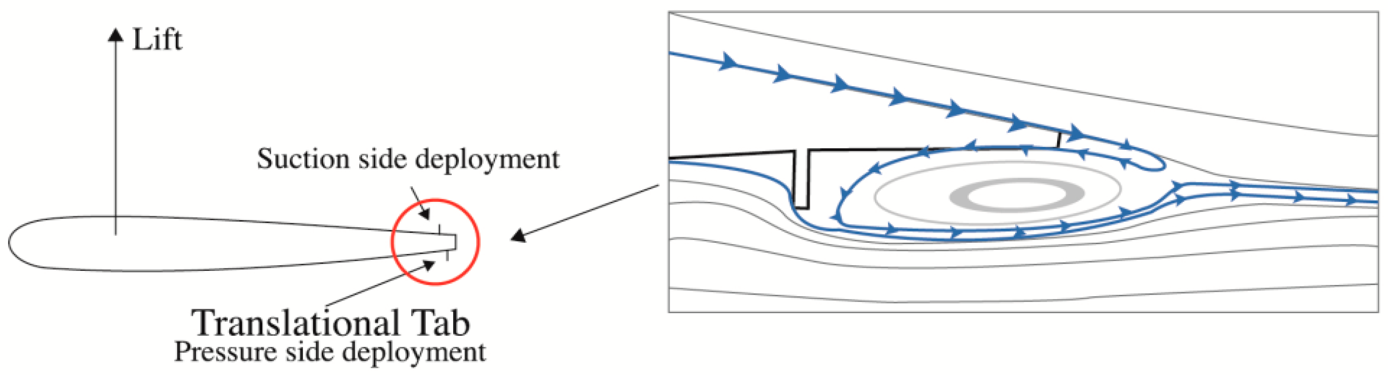
The microtabs (MTs) consist of a small tabs situated close to the trailing edge (TE) of an airfoil, which projects perpendicular to the surface of the airfoil a few percent of the chord length c (usually 1–2%) corresponding to the boundary layer thickness. The potential of MTs was first investigated by van Dam et al. [18]. Baker et al. [19] carried out broad study dedicated to the S809 airfoil with MTs. These MTs jets the flow in the boundary layer away from the blade’s surface, bringing a recirculation zone behind the tab, as can be observed in Figure 1. The MTs affect the airfoil aerodynamics shifting the point of flow separation and, therefore, providing changes in lift. Lift improvement is obtained by implementing the MT downwards (on the pressure side) and lift reduction is obtained by deploying the MT upwards (on the suction side).
The implementation of this device near the airfoil (TE) provokes changes in the flow, causing modifications in the circulation of the flow on the airfoil. The effective camber of the airfoil is modified, promoting changes in the lift and drag forces. Placing a MT at the pressure surface the lift is increased, however if it is placed on the suction, the opposite effect is reached. The main advantages of MTs are: small size, low cost of manufacturing, low power requirements for its activation, and simplicity of the device design. Multiple studies into this topic were made by van Dam et al. [20] and Yen et al. [21], including wind-tunnel experiments in order to determine their optimal height and location.
The aim of the current study is to find the optimal MT position to increase DU91W(2)250 airfoil aerodynamic performance and to investigate its influence on the average power output of a 5 MW Wind turbine. Firstly, a parametric study of a MT mounted on the pressure surface of the airfoil DU91W(2)250 has been carried out and best case has been selected. This airfoil has been selected because it is used on the 5 MW reference wind turbine of the NREL, as described in Jonkman et al. [22]. Second, Blade Element Momentum (BEM) based computations have been performed to investigate the effect of this MTs on the wind turbine power output. The results on the rotor thrust and blade root bending moment are also presented.
2. Parametric Study Based on CFD Calculations
2.1. Numerical Setup
In order to obtain some of the main features of the MT, Computational Fluid Dynamic (CFD) techniques have been employed. Currently, non-commercial and proprietary CFD codes are used to reproduce relatively well any physical problem. In this work, the open source code OpenFOAM has been used for simulating the effects of a MT on a DU91W(2)250. This open source CFD code is an object-oriented library written in C++ to solve computational continuum mechanics problems. One of its advantages is that the user can modify the code to create new solvers and applications as well as freely share the code developed.
The SIMPLE algorithm was employed for the pressure-velocity coupling. The convective terms were discretized with a second order linear-upwind scheme. The discretization of the viscous terms was achieved by means of a second order central-differences linear scheme. The simulations were run fully turbulent. Steady state simulations were carried out and performed with a structured finite-volume flow solver using Reynolds averaged Navier–Stokes (RANS) equations. For these computations the k-ω SST shear stress turbulence model developed by Menter [23] was used due to its superior separated flow performance, as reported by Kral [24] and Gatski [25]. The model is a combination of two models: Wilcox’s k-ω model for near wall regions and the k-ε model for the outer region and in free shear flows. The SST model departs from existing k-ω and k-ε models by way of a modified eddy viscosity definition that results in improved prediction of separated flows. Reynolds-averaged Navier–Stokes calculations with SST turbulence model for various tab configurations applied to an airfoil are presented in Mayda et al. [26]. Figure 2 illustrates the computational setup with the current setting consisting of a DU airfoil. An O-mesh type was designed for the computations with a computational domain radius of 32 times the airfoil chord length R = 32c, which is in the order of the computational size recommended by Sørensen et al. [27] for this type of simulations.
The Reynolds number based on the airfoil chord length of c = 1 m is Re = 7 × 10⁶. The computational setup of the simulations consists of a structured mesh with the first cell height ∆z/c of 1.45 × 10⁻⁶ normalized by the airfoil chord length. The stretching in the chord-wise and normal directions is accomplished by double sided tanh stretching functions based on Vinokur [28] and Thompson et al. [29]. The mesh domain was designed to have a dimensionless distance less than 1 (y+ < 1) on the airfoil wall. An optimized mesh plays a major role in the CFD simulations as the tool that will help the user to discretize the domain. It is important to identify the mesh regions where the results have to be quite accurate as well as to establish a balance between the accuracy of the simulations and the computational cost. Figure 3 shows the cell distribution around the MT and in the near wake of the trailing edge. The wake and the regions where high gradients were expected were accordingly refined. There are certain regions close to the MT in which the velocity gradient changes drastically, which is the reason why those areas are so important.
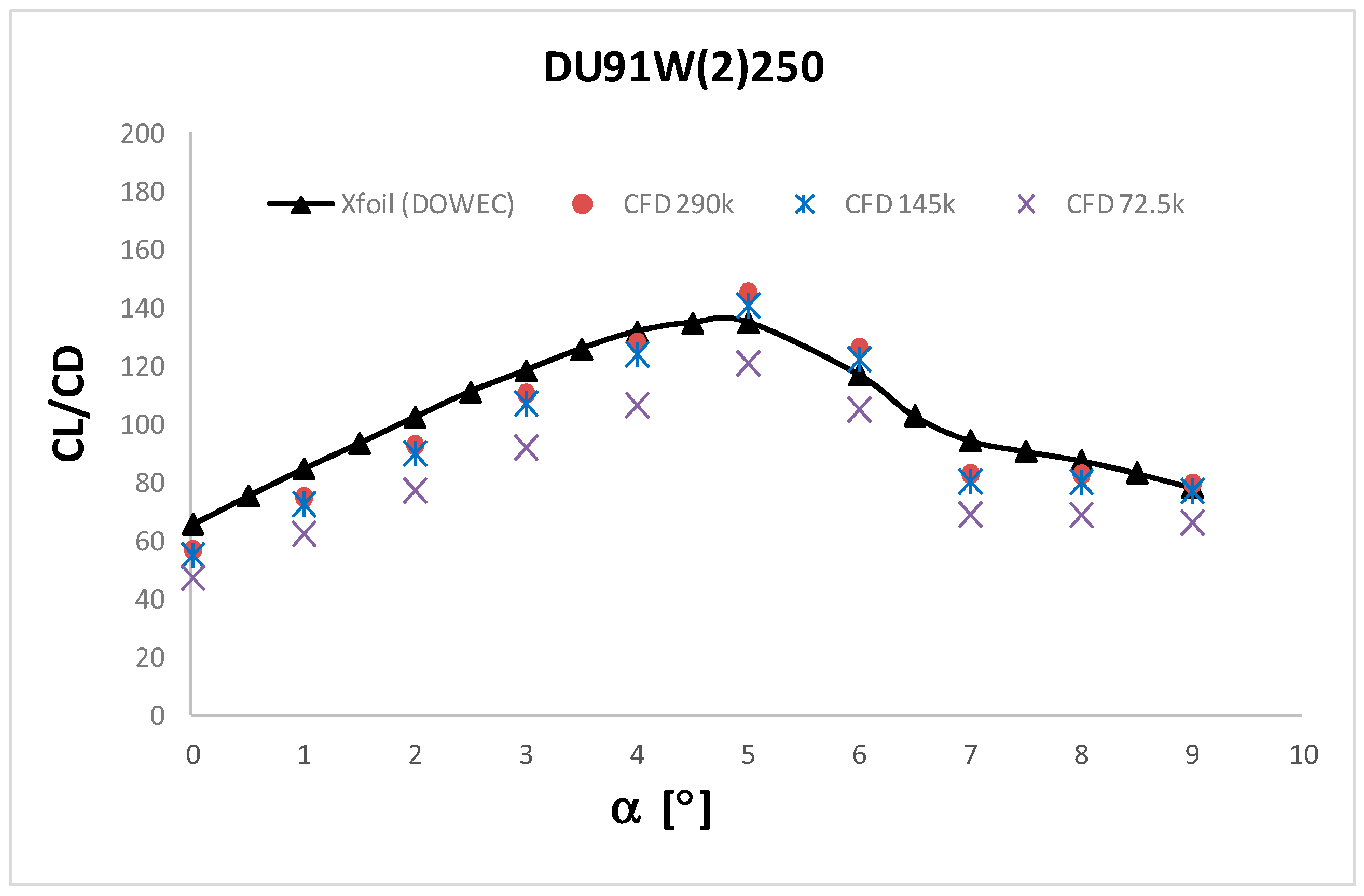
In OpenFoam, both the velocity and the pressure conditions have to be defined at all boundaries, since the velocity-pressure coupling is based on a collocated grid approach. Non-slip boundary condition was set for the airfoil and MT walls. Computational simulations of the DU91(2)250 airfoil without any MT have been carried out and validated against the data obtained by Xfoil from DOWEC project of Kooijman et al. [30] and Lindenburg [31]. The Lift-to-drag ratio was calculated for ten angles of attack (AoA) from α = 0 to α = 9 degrees. Figure 4 shows the results of the CFD computations against the Xfoil results for all angles of attacks of the airfoil.
A mesh independency study was carried out to verify enough grid resolution with three mesh sizes using a refinement ratio of 2. The coarse mesh contains 72,500 cells. For the medium and fine mesh the number of cells is 145,000 and 290,000, respectively. Drag and lift results obtained for the finer mesh are compared with the results of a regular and a coarse mesh. Less than 4% mesh dependency has been found for both drag and lift. The simulations were converged until a satisfactory residual convergence was achieved on the velocities, pressure and turbulence quantities. The CFD results follow reasonable good the trend of DOWEC results. Lift and drag coefficients were calculated according to the Equations (1) and (2), respectively:
The air density was defined by = 1.204 kg/m3 and the free stream velocity, far ahead of the airfoil, corresponds to U∞ = 10.66 m/s. L and D represent the lift and drag forces per unit of area, since the simulations are in 2D.
2.2. Microtab Lay-Out
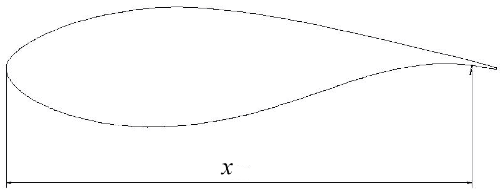
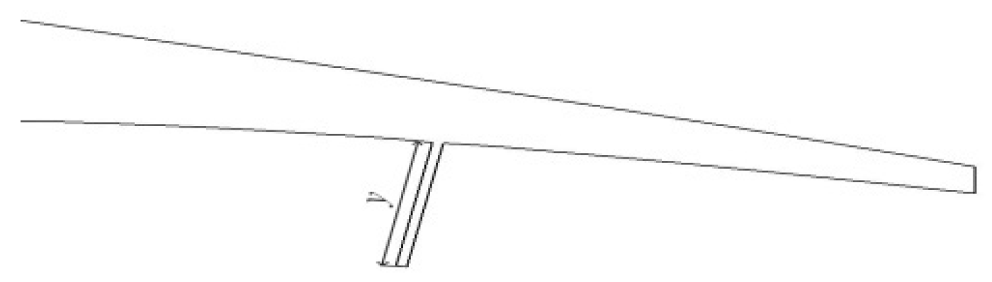
The MT position in the airfoil is sketched in Figure 5 and Figure 6. Dimension x represents the position from the LE and y represents the height of the MT, both in percentage of c. Twelve cases have been established depending on the distance measured respective to the LE in %c (see Table 1). These cases are: 93%c, 94%c, 95%c and 96%c. The MT height relative to the chord length measured in percentage is 1%c, 1.5%c and 2%c. These series of cases has been designed according to the previous studies of Standish et al. [32], Mayda et al. [26] and Yen et al. [21], where the maximum translation was estimated in the order of the boundary layer thickness at the device position: 1–2% of the chord length and the optimal location for a lower surface tab in terms of lift and drag was found to be around 95% of c. The MTs are placed on the pressure surface and have been studied for ten different angles of attack, from 0° to 9°. The combination of all these positions for the MTs gives 120 different cases to study (Ayerdi-Zaton et al. [33]). The airfoil DU91W(2)250 without any flow control device was also simulated to study the influence of the previously described MTs.
2.3. Computational Results
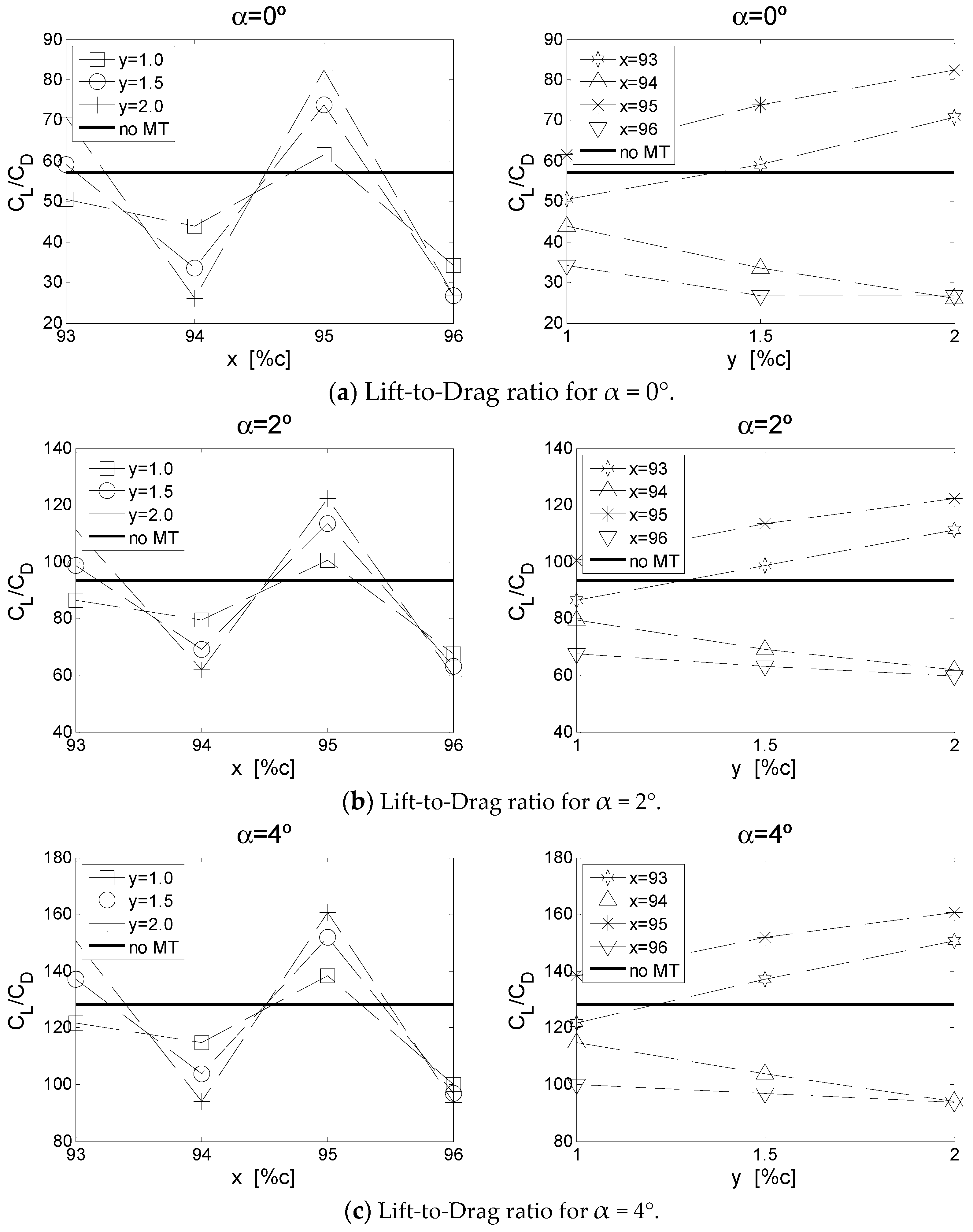
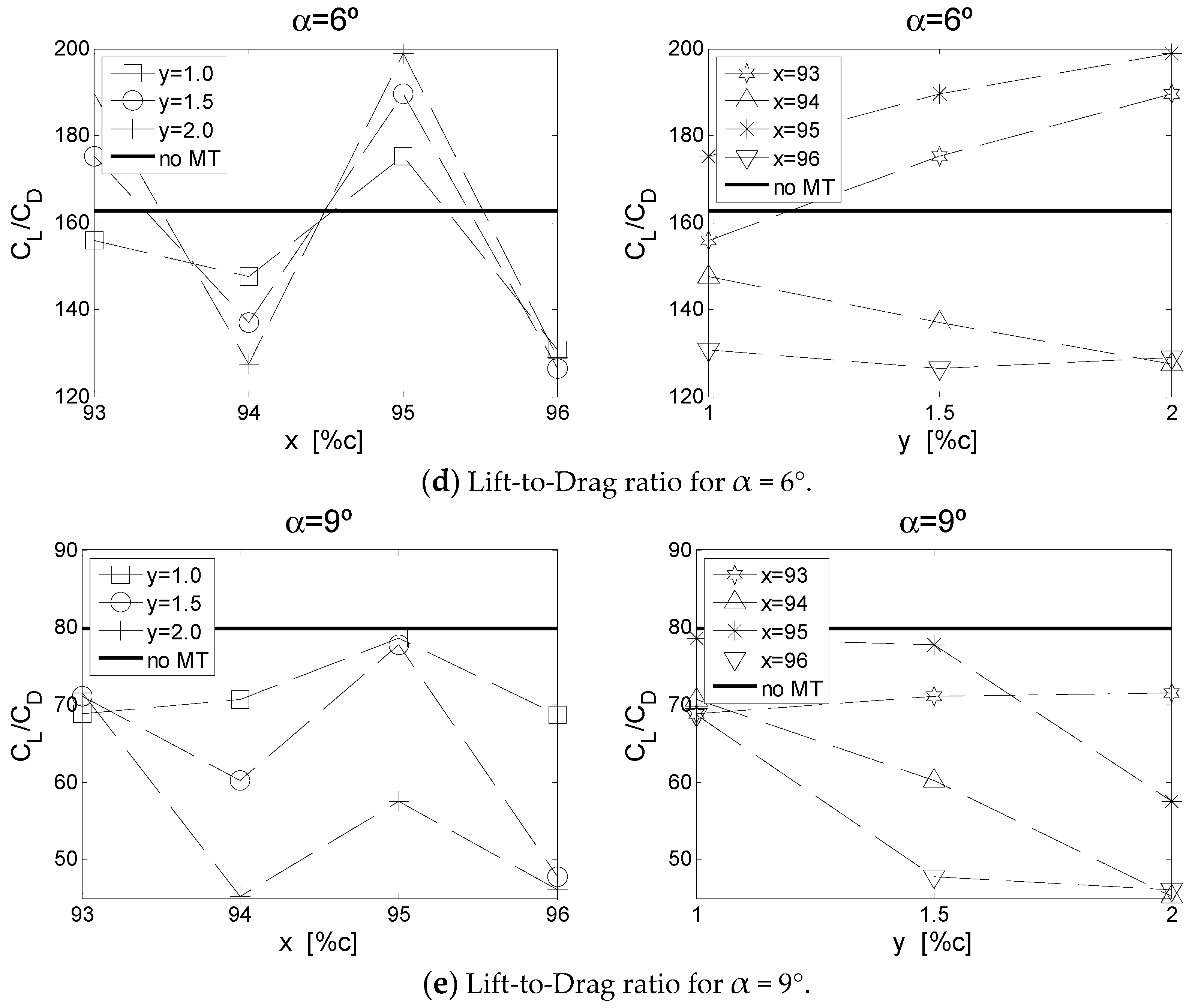
A parametric study has been carried out in order to find the optimal position of the MT on the airfoil DU91W(2)250. Table 1 illustrates the 13 cases studied in the current work. The first case studied is the one with no MT implemented and the other 12 cases with different sizes (y) and position of the MT from the leading edge of the airfoil (x). Each case has been studied for ten different degrees of angle of attack α, in the range from 0° to 9°. Figure 7 illustrates the lift-to-drag ratio CL/CD evolution for every angle α and all MT cases. In the left column the evolution of the CL/CD vs. the location of the MT from the airfoil leading edge x is represented. Right column plots illustrate the CL/CD evolution against the three different heights of the MT y = 1, 1.5 and 2%c. Both x and y parameters are represented in terms of percent of the airfoil chord length c. The Lift-to-drag ratio of the airfoil without MT for each AoA is represented by the black continuous line in each plot.
For the range of angles of attack, from 0° to 9°, the best values of the CL/CD ratio are reached by the cases MT9510, MT9515 and MT9520. However, as can be seen in the left column plots of Figure 7, the highest values are reached around the x = 95% of the chord length. On the right column plots, it is clear again that the best values of the Lift-to-drag ratio are reached by x = 95% of c, and the highest ones by the MT height of y = 2% of c. Therefore, in the range of angles of attack studied in the present work, the best case in terms of Lift-to-drag ratio is the one defined by: x = 95% and y = 2% of c. These results are in concordance previous studies of Yen et al. [21] where it was found that the best place to situate the lower surface tab with respect to lift and drag was around 95%c. According to the classification of Table 1, that case corresponds to DU912250MT9520. The CL/CD ratio achieved in that case, keeps up to the ratio of the clean airfoil represented in Figure 7 with a continuous black line. Figure 8 illustrates the Lift-to-drag ratio values of the case DU912250MT9520 in comparison with the ratios obtained for the clean airfoil.
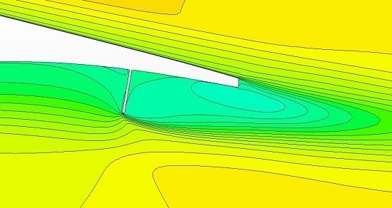
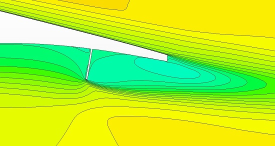
At low AoAs, the increase in the CL/CD ratio due to the microtab MT9520 implementation is clearly visible. However, at the AoA of 9° the CL/CD ratio stays below the CL/CD ratio of the clean airfoil DU91W(2)250. Note that this behavior is repeated by the other cases with different MTs configurations, as shown in Figure 7e. The reason could be found in the fact that at 9° of AoA the airfoil is working near the stall conditions and the CD increases considerably. Since the computations were performed in 2D, three-dimensional effects were neglected. In the studies of Mayda et al. [26] and Zahle et al. [34], a detailed study on the three-dimensional shedding and spanwise flow can be found. Figure 9 represents the streamwise velocity distribution around the MT of the case with the best Lift-to-drag ratio: DU91W(2)250 MT9520. The presence of the tab changes the trailing edge flow development, the so-called Kutta condition, and consequently the effective camber of the airfoils is modified, providing in this case lift enhance. The MT jets the flow in the BL away from the airfoil surface, producing a circulation region behind the tab.
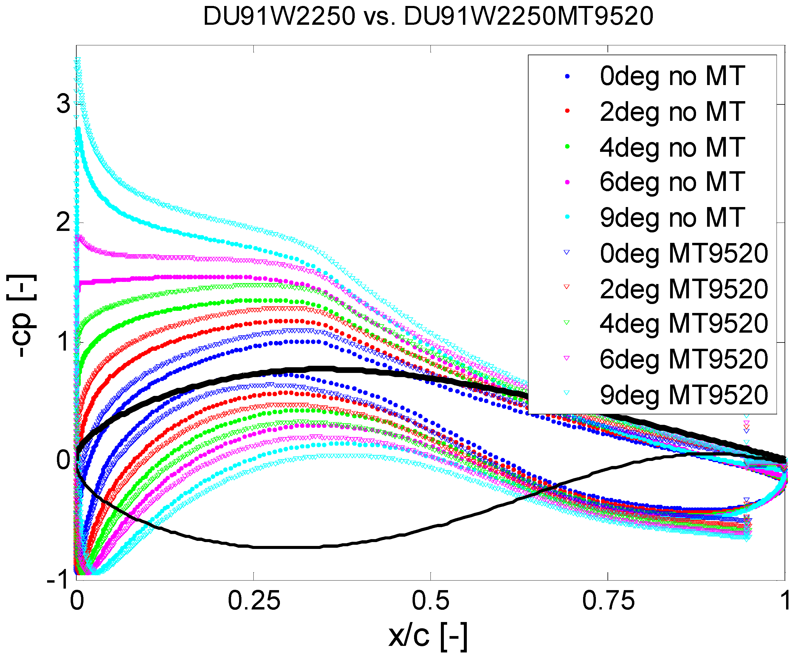
A comparison of the pressure distribution on the surface of the clean airfoil DU91W(2)250 and the airfoil with the best aerodynamic performance in terms of lit-to-drag ratio DU91W(2)250MT9520 is presented in Figure 10. The presence of the MT considerably increases the aft loading of the airfoil and a positive gap between the clean and the microtabed airfoil is clearly visible at all angles of attack. The airfoil shape is sketched by a continuous black line.
3. Wind Speed Model
The wind speed realizations used in the current study, as shown in Figure 11, have been calculated with the TurbSim tool (Kelley et al. [35]). The turbulence model is the Normal Turbulence Model (NTM) following the IEC 61400 norm and the wind speed series have been generated with the following parameters:
- Mean wind speeds in the hub: 5 and 10 m/s;
- Spectral model: IECKAI (B); and
- Hub height: 90 m.
TurbSim uses an adapted version of Veers [36] to generate time series based on spectral representation. The IECKAI (IEC Kaimal) model is defined in IEC 61400-1 2nd ed. [37] and 3rd ed. [38], and assumes neutral atmospheric stability. The spectra for the three wind components, K = u, v, w, are calculated by Equation (3):
where f is the cyclic frequency and LK is an integral scale parameter defined in IEC 61400-1 standard.
The velocity spectra of the IECKAI model are assumed to be invariant across the grid. In practice, a small amount of variation in the u-component standard deviation occurs due to the spatial coherence model. Figure 11 represents the wind speed series used in the present study according to the Normal Turbulence model with 5 m/s, 7.5 m/s and with 10 m/s average velocity, respectively. According to TurbSim user specifications, the first input value is a random seed that must be an integer between −2,147,483,648 and 2,147,483,647 (inclusive). In the current study, three different seeds have been chosen for each wind realizations. Figure 11a–c illustrates the wind patterns generated for each wind speed. The values of Seeds 1–3 have been chosen to obtain different wind patterns and are the same for each average wind speed.
These different wind speed realizations were chosen to investigate the effects of the MTs, since it is a good way to evaluate the wind turbine power output at low and medium wind velocities. Four different cases were considered in the current study. The clean wind turbine was taken as the baseline case, without any device implemented and named DU91W(2)250. According to the matrix presented in Table 2, the cases are different depending on the blade station where the passive devices were implemented. The suffix st means the blade station where the MTs were introduced. According to the airfoil distribution described in [22], stations 8 and 9 were chosen for the present study.
4. Methodology
The primary tools used in the current work to investigate the effects of the passive MTs on the NREL 5 MW Baseline Wind Turbine are engineering models. The NREL 5 MW reference wind turbine is widely used in research studies in the wind energy field since it represents a baseline of the modern and future offshore HAWT. Many investigations have been carried out based on this wind turbine concept including studies about rotor aerodynamics, controls, offshore dynamics and design code development. This concept of a 5 MW wind turbine is based on the data from the DOWEC study [30,31], with a concept from the UpWind project [39]. The airfoils and chord schedule used in the present work are presented in Table 3 and are the same from NREL [22], also adopted from the DOWEC project. The blade airfoil locations, labeled as r (m) in Table 3, are directed along the blade-pitch axis from the rotor center to the blade cross sections. The DU25 airfoil corresponds to the DU91W(2)250. More detailed information on the DU family of airfoils used in the current work can be found in the study made by Timmer [40]. The reported NREL 5 MW airfoil distribution is shown in Figure 12.
Once the lift and drag coefficients are identified for the airfoils along the blades, it is feasible to compute the force distribution. Global loads such as the power output and the root bending moment of the blade can be found by integrating this distribution along the blade span. It is the principle of the BEM method, which will be derived to compute the induction factors a and a’ and thus the loads on a wind turbine. The present procedure is described in the following steps:
- First of all, BEM based computations were carried out in order to characterize the dynamical behavior of the NREL 5 MW wind turbine, including Prandtl’s tip loss factor and Glauert’s correction. The BEM solver was developed and programmed by the authors of the current study based on the numerical iterative approach of Hansen [41]. All the necessary equations were derived and computed based on the steps proposed by the classical blade element momentum method. The usual basic steps for BEM calculations was followed; this is a short schedule:
- Initialization by guessing values of a and a’ values, axial and tangential induction factors, respectively.
- Calculate the flow angle Φ.
- Calculate the local angle of attack α.
- Read off CL (α) and CD (α).
- Compute the normal Cn and tangential Ct load coefficients.
- Re-calculate a and a’.
- State a tolerance for a and a’ and if it has changed more than that tolerance, go to (b) or else finish.
- Compute the local loads.
- Following the specifications of the utility scale multi megawatt wind turbine NREL 5 MW baseline described in [22], all the wind turbine rotor properties were introduced as input characteristics. The polar curves of the airfoil with the MT were taken from best case found in Section 2, which is the DU91W(2)250MT9520 with the MT position from the leading edge at 95% of c and the MT height of 2% of c.
- The surfaces of power coefficient Cp were calculated for all cases of the present study according to the matrix distribution described in Table 2.
- Once the Cp surfaces have been generated, BEM based computations are run for the four cases and the power curve vs. wind speed is calculated to compare the power curve of the clean turbine with the curve of the turbine with the MTs implemented.
- Afterwards, the wind speed realizations explained in Section 3 are introduced to calculate the average wind turbine power output for all cases.
- The results of the average wind turbine power output for all cases and at two different wind speed realizations are compared with the mean power output of the clean wind turbine, the one without any flow control device implemented.
5. Results from BEM Computations
In order to investigate the influence of MTs on the power of the NREL 5 MW reference wind turbine, BEM computations have been carried out following the steps explained in the previous section. The BEM based computations has now been derived and the power has been computed versus the wind speed. Figure 13 illustrates the power curves along the wind speed for the clean case with no passive device implemented into the blade in comparison with the cases with MTs (see Table 2). The power curves of the wind turbine with MTs follow the trends of the curve of the clean wind turbine. However, at the wind speeds before the rated power is achieved, the power output increases slightly in the cases with the MT implemented, as shown in the enlargement view embedded in Figure 13.
Additionally, the average wind turbine power output has been calculated for the clean wind turbine and for the cases with MTs at the wind speed realizations described in Section 3. Equation (4) shows how this average power is calculated:
- ▪
- vj: is the wind speed according to the realizations shown in Figure 11.
- ▪
- Nbins: number of bins per data.
- ▪
- P(vj): power at the wind speed vj.
- ▪
- N(vj): number of data at the wind speed vj.
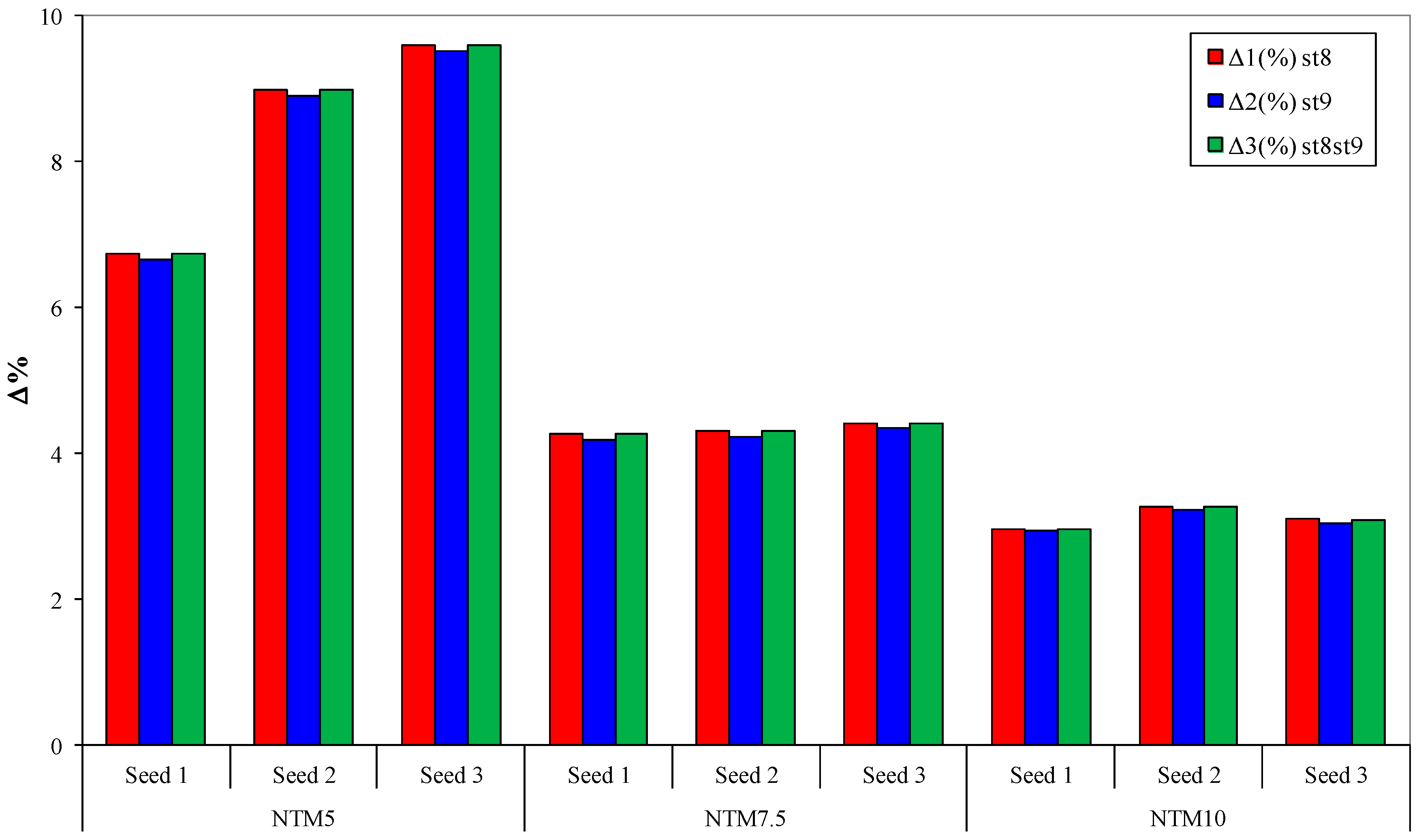
Table 4 shows the results of the power output calculations according to Equation (4). Firstly, the average power has been calculated for the clean wind turbine for the three wind speed realizations illustrated in Figure 11, without any flow control device mounted on the blade. Afterwards, the average wind turbine power was calculated for all cases of MTs distribution described in Table 2 and compared with the clean turbines power values. The symbols denoted by Δ represent the increment of average power in comparison with the clean turbine.
At the wind speed realization of NTM5, the greatest increase in the average power was achieved by the case st8, with a value of 5.3218 × 10⁵ W, which supposes an increase of 9.599% in comparison with the value obtained by the clean wind turbine. Moreover, the other cases with MTs mounted on st9 and st8st9 present a similar increase. At the NTM7.5 wind speed realization, the largest increment average power output was reached by the case with the MTs implemented in the station 8 of the blade, with an increase of the power in compared with the clean wind turbine of 4.425%. At the NTM10 wind speed realization the largest average power value is reached by the case with the MTs mounted on st8 with an increase with respect to the clean case of 3.282%. The largest increases for the three wind speed realization used in the present work have been performed by the case with the MTs in the blade station 8, corresponding to the case DU91W(2)250MT9520st8. Figure 14 illustrates in a bar plot the increments in the power output for every case in comparison with the clean case. The effect of mounting MTs on the blade stations studied in the present work is more significant at low wind speeds than at wind speed close to the nominal power. At those low wind speeds, the MTs can help to increase notably the wind turbine power output performance. Note that even thought the case DU91W(2)250MT9520st8st9 has more MTs mounted along the blade, its power performance in terms of average power output is quite similar in comparison with the other cases with MTs on stations 8 and 9.
After applying the BEM algorithm to all control volumes, the tangential and normal load distribution is known and global parameters such as thrust and bending moment at the root of the blade can be computed. In the current work, the mean values of both thrust and bending moment have been calculated for each wind speed realization. The thrust has been calculated by Equation (5) taking into account the trust distribution along the blade and the bending moment has been determined by Equation (6).
The Prandtl’s tip loss correction factor F has been determined by the Equation (7), for both thrush and bending moment calculations:
The variables used for thrust and bending moment estimations and the corresponding dimensions are shown in Table 5. All calculations are based on the 5 MW reference wind turbine described in [22].
Table 6 represents the mean values of thrust calculations for all MT cases according to the matrix described in Table 2. The thrust was calculated by integrating the thrust distribution along the blade by the Equation (5) for each wind speed realization. Afterwards, the average thrust was determined according to the wind realization duration of Figure 11. The increments in the average thrust of the microtabed blade cases have been illustrated in Table 6 in comparison with the clean case. The average thrust has been experienced an increase in every case with MTs implemented and once again, the case with the MTs mounted on the blade station 8 presents larger increments than the other cases, which is in concordance with the results of power output presented in Figure 14.
The bending moment in the root of the blade has been determined by Equation (6) taking into account the bending moment distribution along the blade. The bending moment in the root of the blade was determined for each wind speed realization and computed along blade according to Equation (6). Afterwards, the mean bending moment was determined according to the wind realization duration of Figure 11. The increments in the average bending moment of the microtabed blade cases have been illustrated in Table 7 in comparison with the clean case. No extraordinary increment in the mean bending moment in the root of the blade has been found. All the increments in the bending moment due to the MTs implementation are acceptable taking into account the increase in the average power output production presented in Figure 14.
6. Conclusions
A parametric study for design and analysis of a MT on an airfoil has been carried out. To that end, 2D computational fluid dynamic simulations have been performed at Reynolds number of Re = 7 × 10⁶. The MT design attributes resulting from the simulations have allowed the sizing and positioning of the passive device based on aerodynamic performance. Comparisons of the CFD simulations and the DOWEC results have been made and verified the effectiveness of the MTs as flow control devices to increase the aerodynamics performance. The case DU91W(2)250MT9520 with the MT positioned at 95% of c and with the height of 2% is the one with the best aerodynamic performance in terms of lift-to-drag ratio. Afterwards, BEM based computations have been carried out to investigate the effects of that designed MT on the power performance of a 5 MW wind turbine. An increase on the average wind turbine power output has been found in the current study due to the implementation of MTs at different blade stations. That increase is more notable for the wind speed realizations with lower average wind speed NTM5. However, that increase is still significant with the wind speed realizations with average speeds of 7.5 m/s NTM7.5 and 10 m/s NTM10. In those cases, the increase in the power output is lower but still important. The best results in terms of average power are reached by the case denoted by DU91W(2)250MT9520st8 with the MTs implemented into the blade station 8. The largest increase in thrust has also been achieved by the case with the MTs mounted on the blade station 8. As expected, the increase in the wind turbine power output due to the MTs implementation leads to an augmentation in the bending moment in the root of the blade. However, this increase in the bending moment is acceptable taking into account the raise in the average power output production achieved by all cases. Moreover, no significant variation in the power increase has been found for the other MT locations st9 and st8st9. Because of the cheaper assembly of MT in only one blade station, the case with the MTs on the station 8 DU91W(2)250MT9520st8 is recommended.
The results of the current study shows that carefully analysis of MT height and location in the pressure surface from the airfoil leading edge, combined with a selection of an appropriate spanwise location on the blade, can yield an effective device flow control system to increase the wind turbine power output.
Acknowledgments
The authors are grateful to the Government of the Basque Country and the University of the Basque Country UPV/EHU through the SAIOTEK (S-PE11UN112) and EHU12/26 research programs, respectively.
Author Contributions
Unai Fernandez-Gamiz made the CFD study and Ekaitz Zulueta developed and programmed the BEM based computations. They also wrote the manuscript. Ana Boyano, Josean A. Ramos-Hernanz and Jose Manuel Lopez-Guede made the thrust and bending calculations and provided constructive instructions in the process of preparing the paper.
Conflicts of Interest
The authors declare no conflict of interest.
References
- Bouzelata, Y.; Altin, N.; Chenni, R.; Kurt, E.; Chenni, R.; Kurt, E. Exploration of optimal design and performance of a hybrid wind-solar energy system. Int. J. Hydrogen Energy 2016, 41, 12497–12511. [Google Scholar] [CrossRef]
- Novosel, T.; Cosic, B.; Puksec, T.; Krajacic, G.; Duic, N.; Mathiesen, B.V.; Lund, H.; Mustafa, M. Integration of renewables and reverse osmosis desalination—Case study for the jordanian energy system with a high share of wind and photovoltaics. Energy 2015, 92, 270–278. [Google Scholar] [CrossRef]
- Komusanac, I.; Cosic, B.; Duic, N. Impact of high penetration of wind and solar PV generation on the country power system load: The case study of croatia. Appl. Energy 2016, 184, 1470–1482. [Google Scholar] [CrossRef]
- Jaume, A.M.; Wild, J. Aerodynamic design and optimization of a high-lift device for a wind turbine airfoil. In New Results in Numerical and Experimental Fluid Mechanics X; German Aerospace Aerodynamics Association: Munich, Germany, 2016; Volume 132, pp. 859–869. [Google Scholar]
- Vaz, J.R.P.; Wood, D.H. Aerodynamic optimization of the blades of diffuser-augmented wind turbines. Energy Convers. Manag. 2016, 123, 35–45. [Google Scholar] [CrossRef]
- Houghton, T.; Bell, K.R.W.; Doquet, M. Offshore transmission for wind: Comparing the economic benefits of different offshore network configurations. Renew. Energy 2016, 94, 268–279. [Google Scholar] [CrossRef]
- Johnson, S.J.; van Dam, C.P. Active Load Control Techniques for Wind Turbines; Technical Report SAND2008-4809; Sandia National Laboratories: Livermore, CA, USA, 2008. [Google Scholar]
- Chow, R.; van Dam, C.P. On the temporal response of active load control devices. Wind Energy 2010, 13, 135–149. [Google Scholar] [CrossRef]
- Taylor, H.D. Summary Report on Vortex Generators; Research Department Report No. R-05280-9; United Aircraft Corporation: East Hartford, CT, USA, 1950. [Google Scholar]
- Liu, Y.; Sun, J.; Tang, Y.M.; Lu, L.P. Effect of slot at blade root on compressor cascade performance under different aerodynamic parameters. Appl. Sci. (Basel) 2016, 6, 421. [Google Scholar] [CrossRef]
- Liu, Y.; Sun, J.; Lu, L. Corner separation control by boundary layer suction applied to a highly loaded axial compressor cascade. Energies 2014, 7, 7994–8007. [Google Scholar] [CrossRef]
- Wood, R.M. Discussion of Aerodynamic Control Effectors Concepts (ACEs) for Future Unmanned Air Vehicles (UAVs). Presented at AIAA’s 1st Conference and Workshop on Unmanned Aerospace Vehicles, Systems, Technologies, and Operations, Portsmouth, VA, USA, 20–22 May 2002. AIAA Paper No. 2002-3494. [Google Scholar]
- Shires, A.; Kourkoulis, V. Application of circulation controlled blades for vertical axis wind turbines. Energies 2013, 6, 3744–3763. [Google Scholar] [CrossRef]
- Xu, H.; Qiao, C.; Ye, Z. Dynamic stall control on the wind turbine airfoil via a co-flow jet. Energies 2016, 9, 429. [Google Scholar] [CrossRef]
- Aramendia-Iradi, I.; Fernandez-Gamiz, U.; Sancho-Saiz, J.; Zulueta-Guerrero, E. State of the art of active and passive flow control devices for wind turbines. DYNA 2016, 91, 512–516. [Google Scholar] [CrossRef]
- Becker, R.; Garwon, M.; Guknecht, C.; Barwolff, G.; King, R. Robust control of separated shear flows in simulation and experiment. J. Process Control 2005, 15, 691–700. [Google Scholar] [CrossRef]
- Macquart, T.; Maheri, A. Integrated aeroelastic and control analysis of wind turbine blades equipped with microtabs. Renew. Energy 2015, 75, 102–114. [Google Scholar] [CrossRef]
- Van Dam, C.; Nakafuji, D.Y.; Bauer, C.; Standish, K.; Chao, D. Computational design and analysis of a microtab based aerodynamic loads control system for lifting surfaces. In Proceedings of the MEMS Components and Applications for Industry, Automobiles, Aerospace, and Communication II, San Jose, CA, USA, 25 January 2003; Volume 4981, pp. 28–39. [Google Scholar]
- Baker, J.P.; Standish, K.J.; van Dam, C.P. Two-dimensional wind tunnel and computational investigation of a microtab modified airfoil. J. Aircr. 2007, 44, 563–572. [Google Scholar] [CrossRef]
- Van Dam, C.P.; van Dam, C.P.; Chow, R.; Zayas, J.R.; Berg, D.E. Computational investigations of small deploying tabs and flaps for aerodynamic load control. Sci. Mak. Torque Wind 2007, 75, 012027. [Google Scholar]
- Yen, D.T.; Van Dam, C.P.; Bräuchle, F.; Smith, R.L.; Collins, S.D. Active Load Control and Lift Enhancement Using MEM Translational Tabs. In Proceedings of the AIAA 2000-2242, Fluids 2000 Conference and Exhibit, Fluid Dynamics and Co-located Conferences, Denver, CO, USA, 19–22 June 2000. [Google Scholar]
- Jonkman, J.; Butterfield, S.; Musial, W.; Scott, G. Definition of a 5 MW Reference Wind Turbine for Offshore System Development; Technical Report NREL/TP-500-38060; National Renewable Energy Laboratory: Golden, CO, USA, 2009. [Google Scholar]
- Menter, F.R. Zonal two equation k-w turbulence models for aerodynamic flows. In Proceedings of the 23rd Fluid Dynamics, Plasmadynamics, and Lasers Conference, Fluid Dynamics and Co-located Conferences, Orlando, FL, USA, 6–9 July 1993; American Institute of Aeronautics and Astronautics: Orlando, FL, USA, 1993. [Google Scholar]
- Kral, L. Recent experience with different turbulence models applied to the calculation of flow over aircraft components. Prog. Aerosp. Sci. 1998, 34, 481–541. [Google Scholar] [CrossRef]
- Gatski, T.B. Turbulence Modeling for Aeronautical Flows, vol. VKI Lecture Series: CFD-Based Aircraft Drag Prediction and Reduction; von Karman Institute for Fluid Dynamics: Brussels, Belgium, 2003. [Google Scholar]
- Mayda, E.A.; van Dam, C.P.; Nakafuji, D. Computational Investigation of Finite Width Microtabs for Aerodynamic Load Control. In Proceedings of the 43rd AIAA Aerospace Sciences Meeting and Exhibit Anonymous, Reno, Nevada, 10–13 January 2005. [Google Scholar]
- Sørensen, N.N.; Mendez, B.; Muñoz, A.; Sieros, G.; Jost, E.; Lutz, T.; Papadakis, G.; Voutsinas, S.; Barakos, G.N.; Colonia, S.; et al. CFD code comparison for 2D airfoil flows. J. Phys. Conf. Ser. 2016, 753, 082019. [Google Scholar] [CrossRef]
- Vinokur, M. On one-dimensional stretching functions for finite-difference calculations. J. Comput. Phys. 1983, 50, 215–234. [Google Scholar] [CrossRef]
- Thompson, J.F.; Warsi, Z.U.A.; Mastin, C.W. Numerical Grid Generation; Elsevier: North-Holland, NY, USA, 1985. [Google Scholar]
- Kooijman, H.J.T.; Lindenburg, C.; Winkelaar, D.; van der Hooft, E.L. DOWEC 6 MW Pre-Design: Aero-Elastic Modeling of the DOWEC 6 MW Pre-Design in PHATAS; Technical Report ECN-CX--01-135, DOWEC 10046_009; Energy Research Center of the Netherlands: Petten, The Netherlands, 2003. [Google Scholar]
- Lindenburg, C. Aeroelastic Modeling of the LMH64-5 Blade; Technical Report DOWEC-02-KL-083/0, DOWEC 10083_001; Energy Research Center of the Netherlands: Petten, The Netherlands, 2002. [Google Scholar]
- Standish, K.; van Dam, C. Computational analysis of a microtab-based aerodynamic load control system for rotor blades. J. Am. Helicopter Soc. 2005, 50, 249–258. [Google Scholar] [CrossRef]
- Ayerdi-Zaton, J.; Fernandez-Gamiz, U.; Zulueta, E.; Lopez-Guede, J.M.; Ramos, J.A. Computational study of a microtab deployed on a DU airfoil. In Proceedings of the European Conference on Renewable Energy Systems ECRES, Istanbul, Turkey, 28–31 August 2016. [Google Scholar]
- Zahle, F.; Sørensen, N.N.; Graham, J.M.R. Computational study of the risø B1-24 wind turbine profile fitted with gurney flaps. In Proceedings of the EWEA Special Topic Conference, London, UK, 22–25 November 2004. [Google Scholar]
- Kelley, N.; Jonkman, B. NWTC Computer-Aided Engineering Tools (TurbSim). 2012. Available online: http://wind.nrel.gov/designcodes/preprocessors/turbsim/ (accessed on 17 June 2016).
- Veers, P.S. Three-Dimensional Wind Simulation; Technical Report SAND88-0152; Sandia National Laboratories: Albuquerque, NM, USA, 1988. [Google Scholar]
- IEC 61400-1. Wind Turbine Generator Systems-Part 1: Safety Requirements, 2nd ed.; Technical Report; International Electrotechnical Commission: Geneva, Switzerland, 1999. [Google Scholar]
- IEC 61400-1. Wind Turbines-Part 1: Design Requirements, 3rd ed.; Technical Report; International Electrotechnical Commission: Geneva, Switzerland, 2005. [Google Scholar]
- Nijssen, R. WMC5 MW Laminate Lay-Out of Reference Blade for WP 3: Upwind WMC5 MW 374 Laminate Data, Review 1; Knowledge Centre Wind Turbine Materials and Constructions: Wieringerwerf, The Netherlands, 2007. [Google Scholar]
- Timmer, W.A.; van Rooij, R.P.J.O.M. Summary of the delft university wind turbine dedicated airfoils. J. Sol. Energy Eng. Trans. ASME 2003, 125, 488–496. [Google Scholar] [CrossRef]
- Hansen, M.O.L. Aerodynamics of Wind Turbines; Earthscan Publications Ltd.: London, UK, 2015. [Google Scholar]
Figure 1.
Microtabs (MT) concept and enlargement view of the streamlines around the MT mounted on the pressure side of an airfoil [15].
Figure 1.
Microtabs (MT) concept and enlargement view of the streamlines around the MT mounted on the pressure side of an airfoil [15].

Figure 2.
Computational domain.
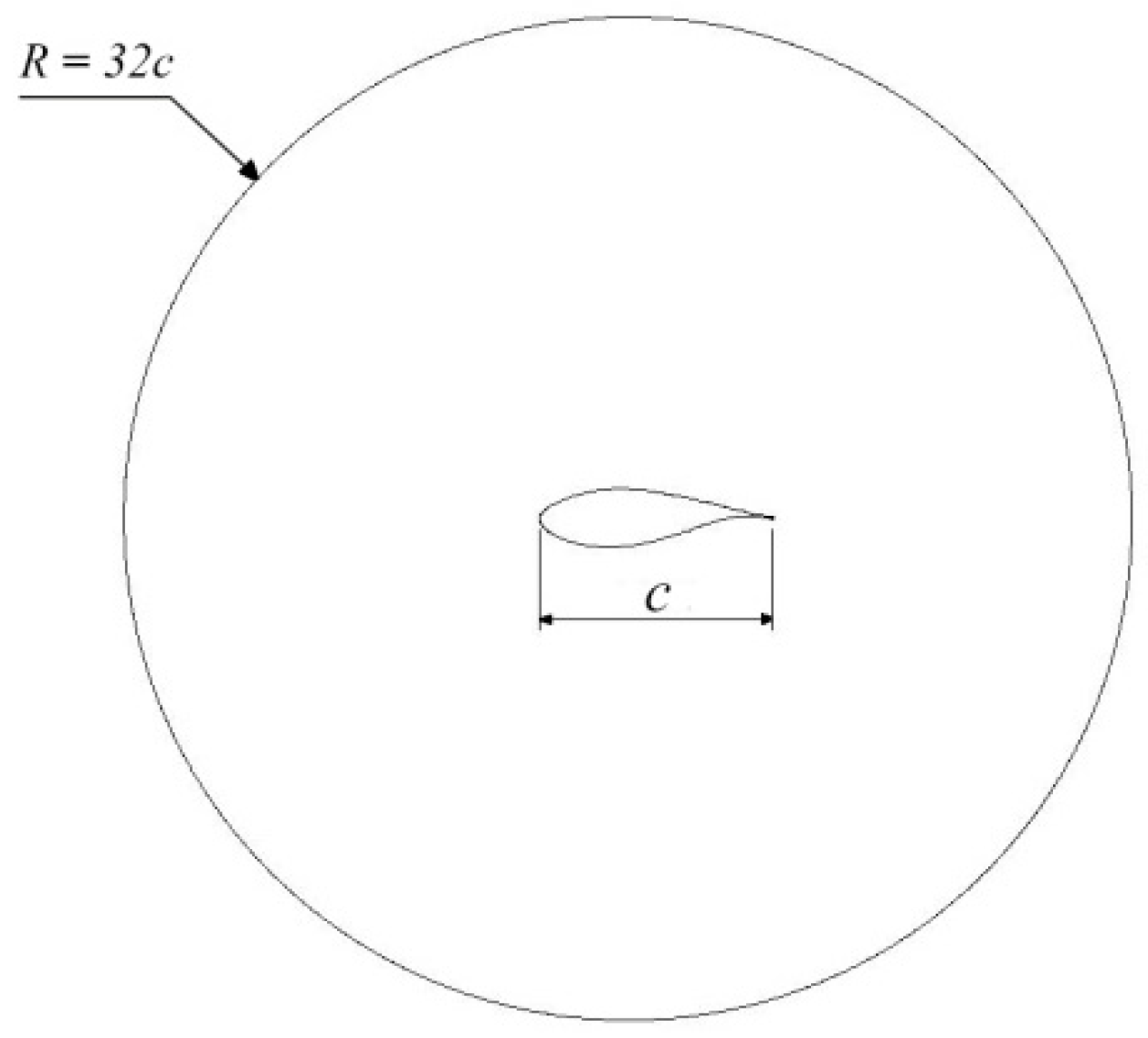
Figure 3.
Mesh distribution on the airfoil the trailing edge (TE).
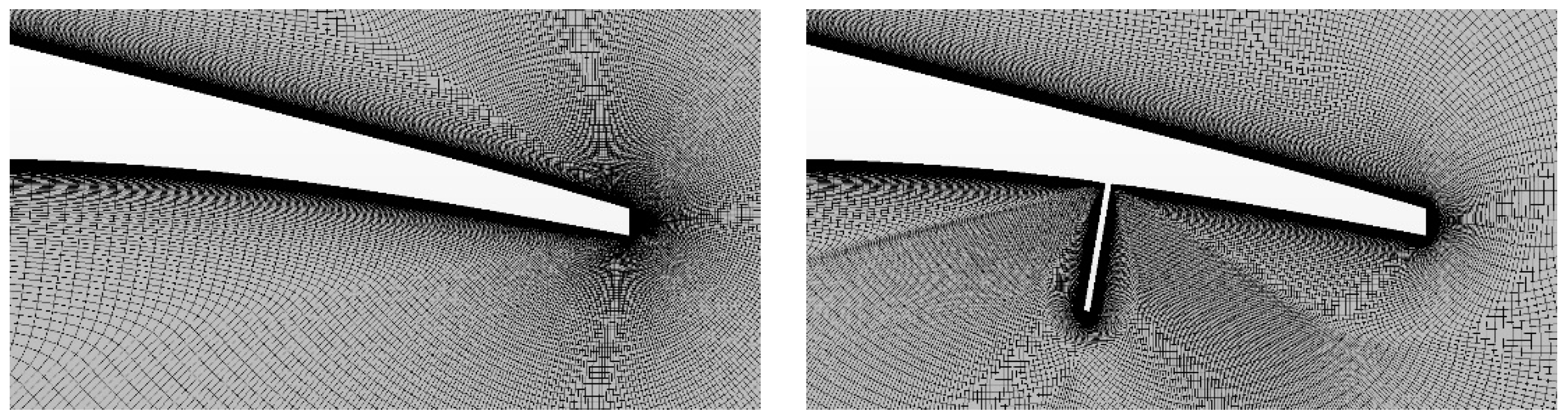
Figure 4.
CL/CD ratio comparison from α = 0° to 9°.

Figure 5.
Relative position of the MT from the leading edge (LE).

Figure 6.
Height of the MT.

Figure 7.
Lift-to-Drag ratio (CL/CD) for the range of α studied in the present work. Right side plots represent the CL/CD evolution against the MT height y. The evolution of the CL/CD along the location of the MT from the leading edge x is represented in the left side.
Figure 7.
Lift-to-Drag ratio (CL/CD) for the range of α studied in the present work. Right side plots represent the CL/CD evolution against the MT height y. The evolution of the CL/CD along the location of the MT from the leading edge x is represented in the left side.


Figure 8.
Lift-to-Drag ratio comparison between the clean airfoil and the case named DU91W(2)250MT9520.
Figure 8.
Lift-to-Drag ratio comparison between the clean airfoil and the case named DU91W(2)250MT9520.
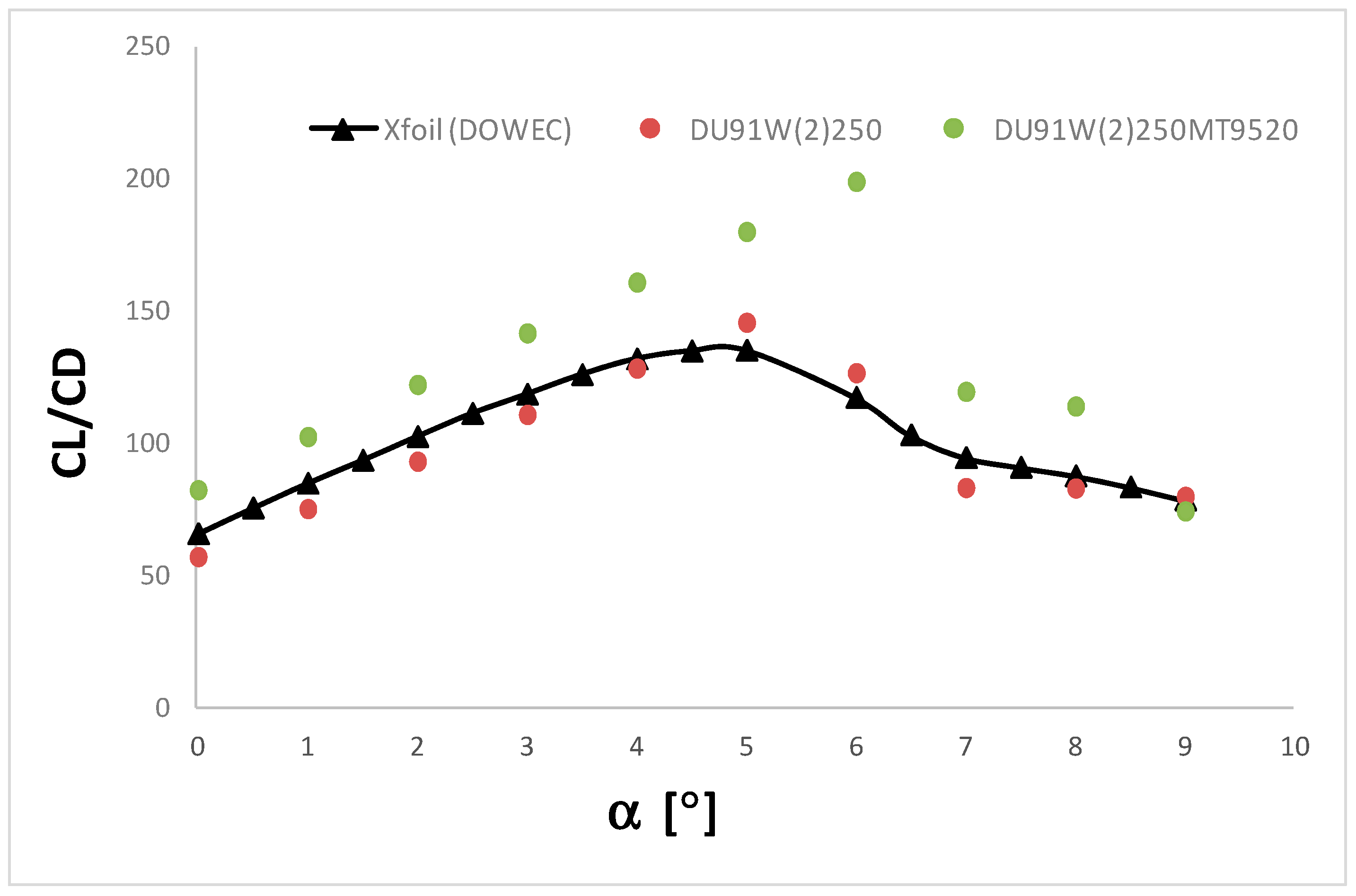
Figure 9.
Streamwise velocity fields of the case DU91W(2)250MT9520 at angles of attack α = 0°, 2°, 4°, 6° and 9°.
Figure 9.
Streamwise velocity fields of the case DU91W(2)250MT9520 at angles of attack α = 0°, 2°, 4°, 6° and 9°.
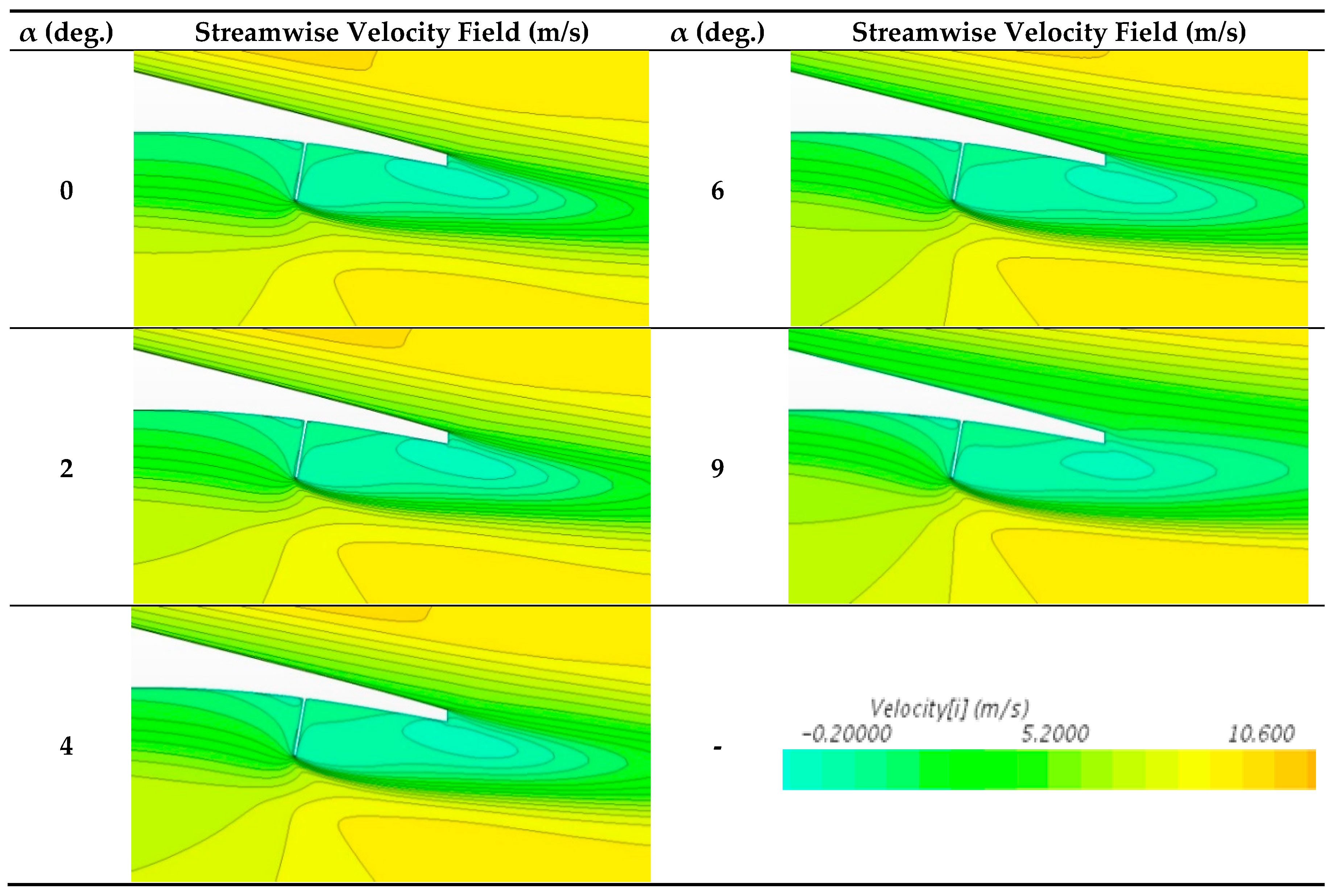
Figure 10.
Pressure coefficient cp comparison between the clean airfoil DU91W(2)250 and the best case DU91W(2)250MT9520 at angles of attack α = 0°, 2°, 4°, 6° and 9°.
Figure 10.
Pressure coefficient cp comparison between the clean airfoil DU91W(2)250 and the best case DU91W(2)250MT9520 at angles of attack α = 0°, 2°, 4°, 6° and 9°.

Figure 11.
Wind speed realization at different average wind speeds.
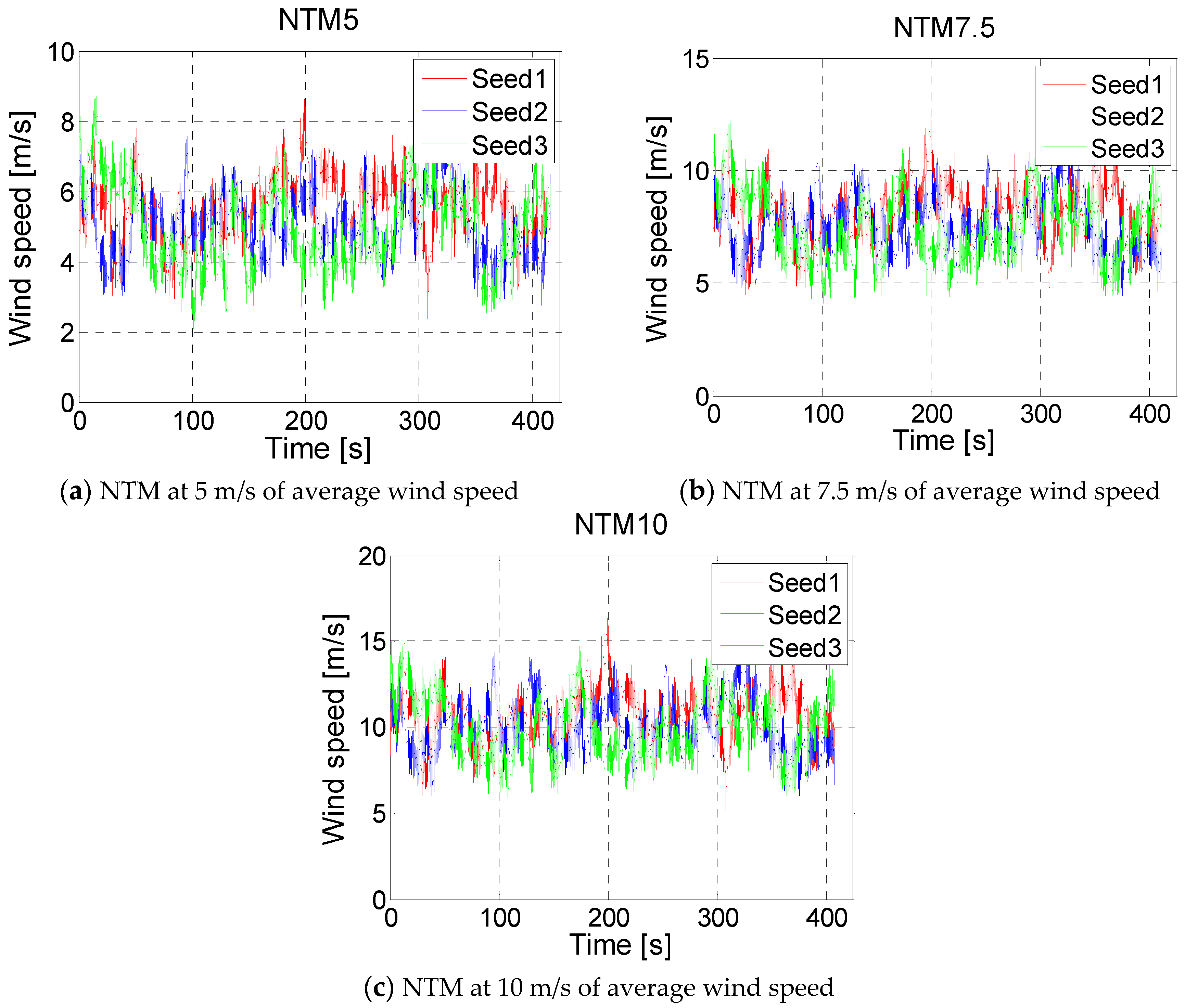
Figure 12.
Sketch of the airfoil distribution along the blade (not to scale) of the NREL 5 MW wind turbine according to [22].
Figure 12.
Sketch of the airfoil distribution along the blade (not to scale) of the NREL 5 MW wind turbine according to [22].
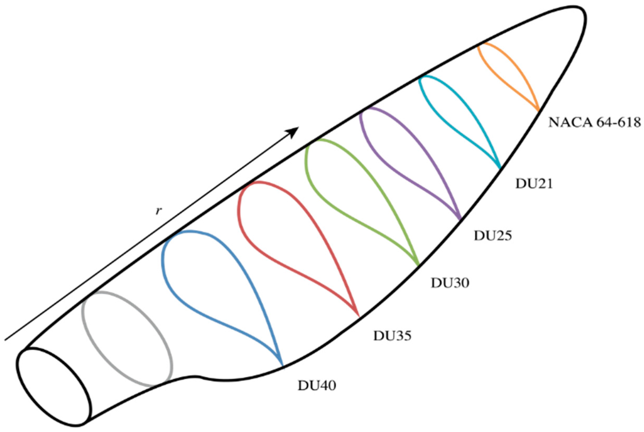
Figure 13.
Comparison of the power curves of the clean turbine with the cases with the MT implemented.
Figure 13.
Comparison of the power curves of the clean turbine with the cases with the MT implemented.
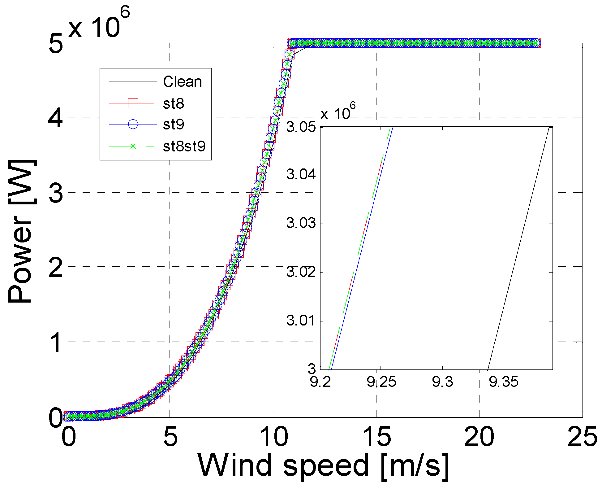
Figure 14.
Average wind turbine power output increases for all wind speed realizations of the microtabed wind turbine in comparison with the clean one.
Figure 14.
Average wind turbine power output increases for all wind speed realizations of the microtabed wind turbine in comparison with the clean one.

Table 1.
Case names and MT dimensions.
| Case Name | x (%c) | y (%c) |
|---|---|---|
| DU91W(2)250 | no MT | no MT |
| DU91W(2)250MT9310 | 93 | 1.0 |
| DU91W(2)250MT9315 | 93 | 1.5 |
| DU91W(2)250MT9320 | 93 | 2.0 |
| DU91W(2)250MT9410 | 94 | 1.0 |
| DU91W(2)250MT9415 | 94 | 1.5 |
| DU91W(2)250MT9420 | 94 | 2.0 |
| DU91W(2)250MT9510 | 95 | 1.0 |
| DU91W(2)250MT9515 | 95 | 1.5 |
| DU91W(2)250MT9520 | 95 | 2.0 |
| DU91W(2)250MT9610 | 96 | 1.0 |
| DU91W(2)250MT9615 | 96 | 1.5 |
| DU91W(2)250MT9620 | 96 | 2.0 |
Table 2.
Cases studied according to MT span distribution along the blade.
| TEST CASES | st8 | st9 |
|---|---|---|
| DU91W(2)250 | no MT | no MT |
| DU91W(2)250MT9520st8 | X | - |
| DU91W(2)250MT9520st9 | - | X |
| DU91W(2)250MT9520st8st9 | X | X |
Table 3.
Airfoil distribution on the Blade.
| Station | r (m) | Airfoil |
|---|---|---|
| 1 | 2.8667 | Cylinder1 |
| 2 | 5.6000 | Cylinder1 |
| 3 | 8.3333 | Cylinder2 |
| 4 | 11.7500 | DU40 |
| 5 | 15.8500 | DU35 |
| 6 | 19.9500 | DU35 |
| 7 | 24.0500 | DU30 |
| 8 | 28.1500 | DU25 |
| 9 | 32.2500 | DU25 |
| 10 | 36.3500 | DU20 |
| 11 | 40.4500 | DU20 |
| 12 | 44.5500 | NACA64XX |
| 13 | 48.6500 | NACA64XX |
| 14 | 52.7500 | NACA64XX |
| 15 | 56.1667 | NACA64XX |
| 16 | 58.9000 | NACA64XX |
| 17 | 61.6333 | NACA64XX |
Table 4.
Average wind turbine power output for the clean wind turbine in comparison with the microtabed wind turbine cases. Calculations have been made at three different wind speed realizations, NTM5, NTM7.5 and NTM10. Δ means the average power variation with respect to the clean case.
Table 4.
Average wind turbine power output for the clean wind turbine in comparison with the microtabed wind turbine cases. Calculations have been made at three different wind speed realizations, NTM5, NTM7.5 and NTM10. Δ means the average power variation with respect to the clean case.
| CLEAN (W) | st8 (W) | Δ1 (%) | st9 (W) | Δ2 (%) | st8st9 (W) | Δ3 (%) | ||
|---|---|---|---|---|---|---|---|---|
| NTM5 | Seed 1 | 639,653 | 682,736 | 6.735 | 682,247 | 6.659 | 682,731 | 6.734 |
| Seed 2 | 498,572 | 543,347 | 8.981 | 542,959 | 8.903 | 543,339 | 8.979 | |
| Seed 3 | 485,570 | 532,180 | 9.599 | 531,780 | 9.517 | 532,154 | 9.594 | |
| NTM7.5 | Seed 1 | 2,043,199 | 2,130,449 | 4.270 | 2,128,954 | 4.197 | 2,130,449 | 4.270 |
| Seed 2 | 1,712,749 | 1,786,646 | 4.315 | 1,785,376 | 4.240 | 1,786,641 | 4.314 | |
| Seed 3 | 1,665,902 | 1,739,621 | 4.425 | 1,738,406 | 4.352 | 1,739,603 | 4.424 | |
| NTM10 | Seed 1 | 4,053,501 | 4,174,148 | 2.976 | 4,172,666 | 2.940 | 4,174,110 | 2.975 |
| Seed 2 | 3,565,184 | 3,682,177 | 3.282 | 3,680,524 | 3.235 | 3,682,172 | 3.281 | |
| Seed 3 | 3,417,900 | 3,524,200 | 3.110 | 3,522,500 | 3.060 | 3,523,800 | 3.098 |
Table 5.
Thrust and bending moment calculations variables.
| Variable | Name | Units |
|---|---|---|
| Vo | wind speed | m/s |
| ai | axial induction factor | - |
| a'i | tangential induction factor | - |
| ri | airfoil spanwise position (radius) | m |
| w | rotor rotational speed | rad/s |
| ρ | air density | Kg/m3 |
| Φ | flow angle | rads |
| ci | airfoil chord length | m |
| dT | thrust on the annular element | N |
| dM | root bending moment | Nm |
| B | number of blades | - |
| R | rotor radius | m |
Table 6.
Mean values of the thrust calculations for the cases with MTs in comparison with the case with no device implemented.
Table 6.
Mean values of the thrust calculations for the cases with MTs in comparison with the case with no device implemented.
| CLEAN (N) | st8 (N) | Δ1 (%) | st9 (N) | Δ2 (%) | st8st9 (N) | Δ3 (%) | ||
|---|---|---|---|---|---|---|---|---|
| NTM5 | Seed 1 | 187,634 | 188,168 | 0.284 | 188,158 | 0.279 | 188,166 | 0.283 |
| Seed 2 | 160,211 | 160,670 | 0.287 | 160,662 | 0.282 | 160,661 | 0.281 | |
| Seed 3 | 155,155 | 155,599 | 0.286 | 155,594 | 0.283 | 155,590 | 0.280 | |
| NTM7.5 | Seed 1 | 398,168 | 399,301 | 0.285 | 399,283 | 0.280 | 399,299 | 0.284 |
| Seed 2 | 352,561 | 353,563 | 0.284 | 353,545 | 0.279 | 353,562 | 0.284 | |
| Seed 3 | 342,486 | 343,461 | 0.285 | 343,449 | 0.281 | 343,452 | 0.282 | |
| NTM10 | Seed 1 | 570,742 | 572,303 | 0.273 | 572,283 | 0.270 | 572,295 | 0.272 |
| Seed 2 | 534,179 | 535,603 | 0.267 | 535,584 | 0.263 | 535,595 | 0.265 | |
| Seed 3 | 511,960 | 513,324 | 0.266 | 513,302 | 0.262 | 513,307 | 0.263 |
Table 7.
Mean values of the bending moment at the root of the blade.
| CLEAN (Nm) | st8 (Nm) | Δ1 (%) | st9 (Nm) | Δ2 (%) | st8st9 (Nm) | Δ3 (%) | ||
|---|---|---|---|---|---|---|---|---|
| NTM5 | Seed 1 | 8109216 | 8126789 | 0.217 | 8126853 | 0.218 | 8126886 | 0.218 |
| Seed 2 | 6924009 | 6939014 | 0.217 | 6939069 | 0.218 | 6939076 | 0.218 | |
| Seed 3 | 6705529 | 6720060 | 0.217 | 6720113 | 0.218 | 6720113 | 0.218 | |
| NTM7.5 | Seed 1 | 17207278 | 17244535 | 0.217 | 17244704 | 0.218 | 17244704 | 0.218 |
| Seed 2 | 15237018 | 15270036 | 0.217 | 15270173 | 0.218 | 15270173 | 0.218 | |
| Seed 3 | 14801073 | 14833130 | 0.217 | 14833251 | 0.217 | 14833310 | 0.218 | |
| NTM10 | Seed 1 | 24598692 | 24644696 | 0.187 | 24644937 | 0.188 | 24644937 | 0.188 |
| Seed 2 | 23036435 | 23079692 | 0.188 | 23079743 | 0.188 | 23079651 | 0.188 | |
| Seed 3 | 22072422 | 22113547 | 0.186 | 22113587 | 0.187 | 22113697 | 0.187 |
© 2017 by the authors. Licensee MDPI, Basel, Switzerland. This article is an open access article distributed under the terms and conditions of the Creative Commons Attribution (CC BY) license (http://creativecommons.org/licenses/by/4.0/).
Share and Cite
MDPI and ACS Style
Fernandez-Gamiz, U.; Zulueta, E.; Boyano, A.; Ramos-Hernanz, J.A.; Lopez-Guede, J.M. Microtab Design and Implementation on a 5 MW Wind Turbine. Appl. Sci. 2017, 7, 536. https://doi.org/10.3390/app7060536
AMA Style
Fernandez-Gamiz U, Zulueta E, Boyano A, Ramos-Hernanz JA, Lopez-Guede JM. Microtab Design and Implementation on a 5 MW Wind Turbine. Applied Sciences. 2017; 7(6):536. https://doi.org/10.3390/app7060536
Chicago/Turabian StyleFernandez-Gamiz, Unai, Ekaitz Zulueta, Ana Boyano, Josean A. Ramos-Hernanz, and Jose Manuel Lopez-Guede. 2017. "Microtab Design and Implementation on a 5 MW Wind Turbine" Applied Sciences 7, no. 6: 536. https://doi.org/10.3390/app7060536
Note that from the first issue of 2016, this journal uses article numbers instead of page numbers. See further details here.