Article

Cycling Segments Multimodal Analysis and Classification Using Neural Networks

1
Department of Computing and Control Engineering, University of Chemistry and Technology in Prague, 166 28 Prague, Czech Republic
2
Czech Institute of Informatics, Robotics and Cybernetics, Czech Technical University in Prague, 166 36 Prague, Czech Republic
3
Faculty of Applied Informatics, Tomas Bata University in Zlín, 760 05 Zlín, Czech Republic
4
Department of Neurology, Faculty of Medicine in Hradec Králové, Charles University, 500 05 Prague, Czech Republic
*
Author to whom correspondence should be addressed.
Appl. Sci. 2017, 7(6), 581; https://doi.org/10.3390/app7060581
Submission received: 21 April 2017 / Revised: 14 May 2017 / Accepted: 31 May 2017 / Published: 4 June 2017

Abstract

:
This paper presents methodology for the processing of GPS and heart rate signals acquired during long-term physical activities. The data analysed include geo-positioning and heart rate multichannel signals recorded for 272.2 h of cycling across the Andes mountains over a 5694-km long expedition. The proposed computational methods include multimodal data de-noising, visualization, and analysis in order to determine specific biomedical features. The results include the correspondence between the heart rate and slope for downhill and uphill cycling and the mean heart rate evolution on flat segments: a regression coefficient of 0 . 014 bpm/h related to time and 6 . 3 bpm/km related to altitude. The classification accuracy of selected cycling features by neural networks, support vector machine, and k-nearest neighbours methods is between 91.3% and 98.6%. The proposed methods allow the analysis of data during physical activities, enabling an efficient human–machine interaction.

Graphical Abstract

1. Introduction

Recently developed computational technologies enable the use of general methods of digital signal processing and computational intelligence for the analysis of multimodal signals for motion monitoring and for the evaluation of physical activities [1,2,3,4,5,6], fitness level [7], or rehabilitation progress. Data fusion of signals recorded with specific biosensors, positioning systems [8,9], and video cameras has a wide range of applications in detecting moving objects, in diagnosing neurological or motion disorders, and in the development of assisted living technologies [10,11,12].
The present paper is devoted to the analysis of cycling data acquired with a global positioning system (GPS) [13,14,15,16,17] used to record the spatial location of a cyclist using his longitude, latitude, and altitude, together with his heart rate [18]. Figure 1 presents a data segment selected from the whole 5694-km-long cycling route across the Andes mountains that provided data for the long-term analysis of the fitness level in different route conditions and the altitude profile. Figure 2 presents details of this cycling route segment.
The proposed method is based upon the statistical processing of the observed multichannel signals as well as their filtering and analysis in moving windows of selected lengths to find the time-dependence of the fitness level with the trajectory of the route profile. The developed graphical user interface (GUI) constitutes a general framework for the global and local monitoring of GPS data [19,20] combined with the projection of these data onto the associated mapping region.
GPS monitoring constitutes a general environment that is useful in many applications, allowing remote object detection and motion analysis [21,22,23,24,25] using specific signal and image processing methods [26,27,28,29,30]. Advanced algorithms allow the application of systems that can adapt themselves [31] according to changing environments in many cases.

2. Methods

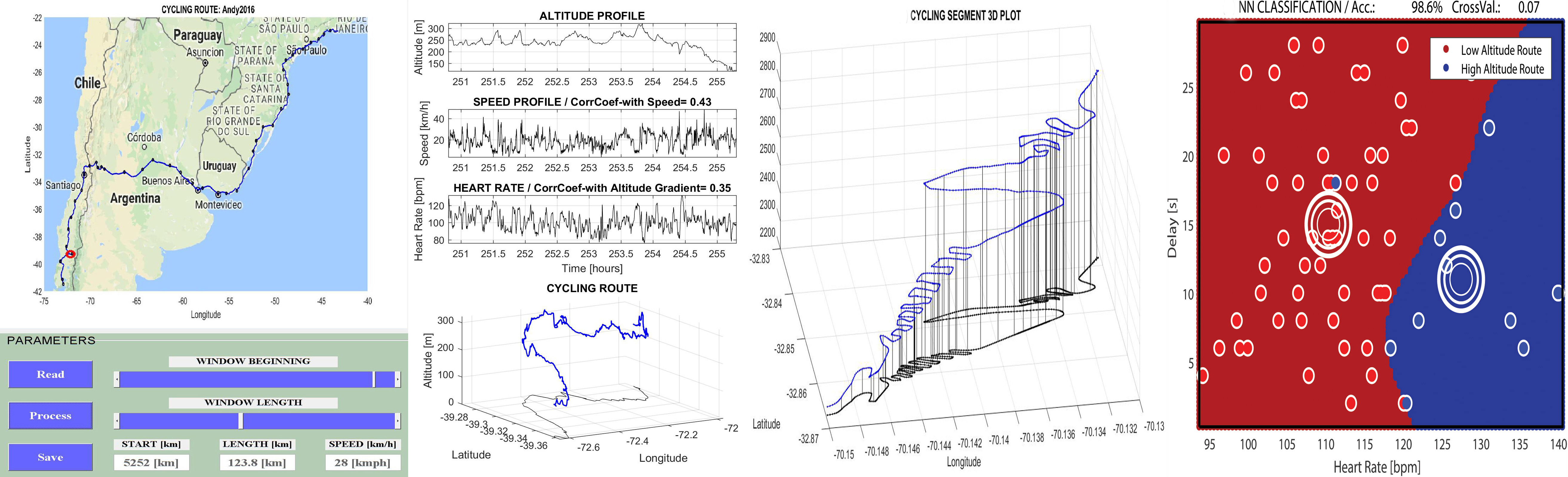
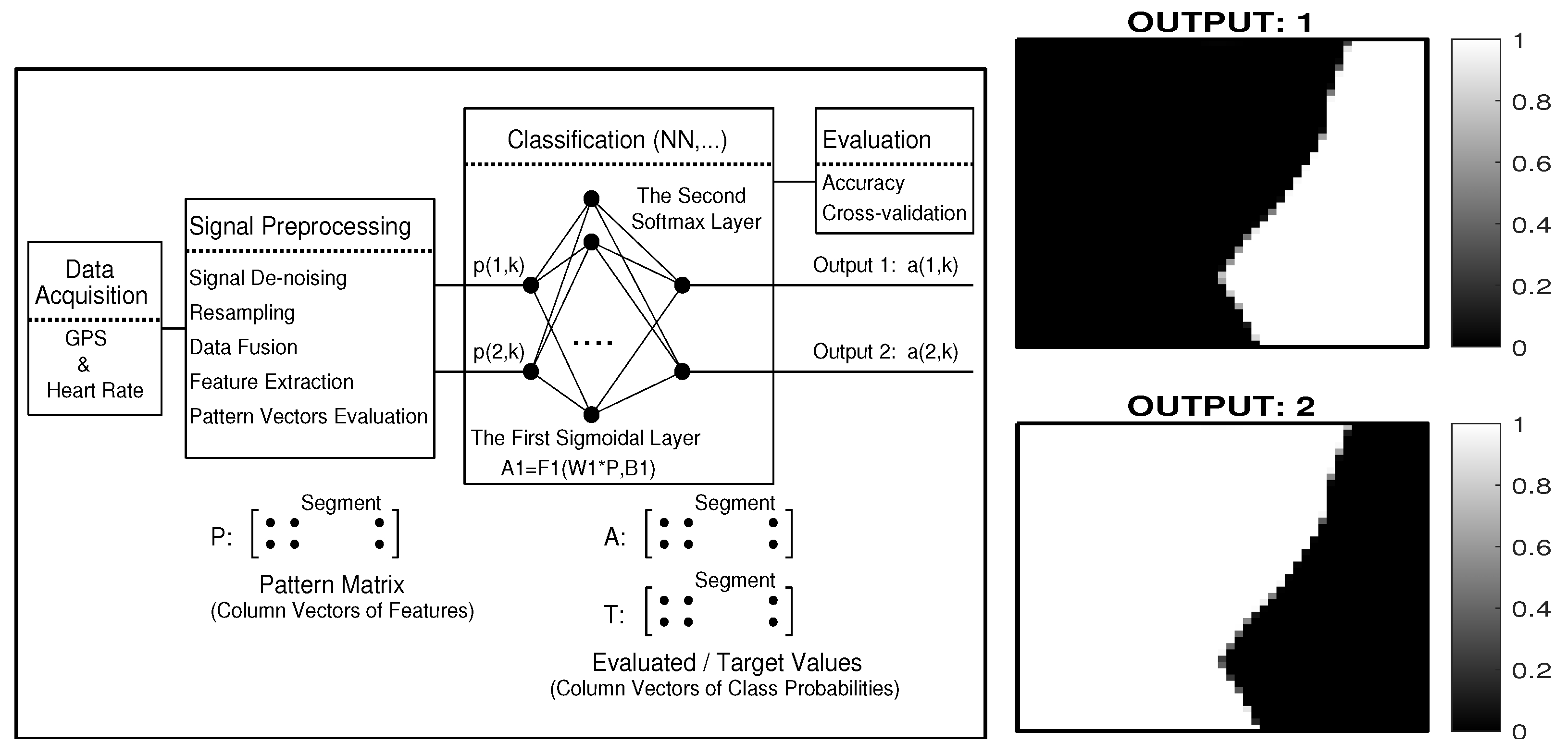
2.1. Data Acquisition

Figure 1 presents a map of the cycling expedition that enabled the data acquisition during the 5694 km cycling route divided into 48 segments, as specified in Table 1 and Supplement 1. Supplement 2 contains a video record of a selected cycling segment specified in Figure 2. Multimodal GPS and heart rate data recorded during the route are presented in Figure 3. Excluding stop-overs, it is possible to summarize that the cycling took 272.2 h, with an average speed of 20.9 km per hour and an average segment length of 118.6 km.
The proposed graphical user interface presented in Figure 1 allows the selection and analysis of any route segment with the chosen starting window position and its length. Figure 2 presents a more detailed 10 km-long segment in the Andes mountains recorded over 28 min of downhill cycling. Data fusion of the recorded data segment with the corresponding Google map region is also presented in Figure 2. Supplement 3 includes all data recorded during the cycling expedition and the MATLAB program to run this GUI.
All GPS and heart rate (HR) data were recorded with a variable sampling period, changing from 1 to 22 s (a sampling rate of 0.05–1 Hz). After the initial processing, they were resampled to a fixed sampling period of 2 s. The resulting matrix of five columns (time, GPS longitude, GPS latitude, GPS altitude, and heart rate) and 490,037 rows (representing 272.2 h of cycling) was then used for further mathematical processing and data analysis.

2.2. Data Processing

The main items of the multichannel GPS and heart rate cycling data analysis and classification are presented in Figure 4. Data acquisition and the following processing steps included:
  • transformation of the data recorded in GPX format into the CSV format and their export to the appropriate (MATLAB) computational and visualization environment;
  • interconnection of all data segments and exclusion of all stops longer than a selected threshold;
  • rejection of gross errors, de-noising of all recorded signals, and their resampling with uniform sampling period, allowing data fusion for the following mathematical processing;
  • interconnection of recorded GPS data with the Google map region;
  • data segmentation using windows of the selected length.
The data analysis included the following steps:
  • selection of windows fulfilling chosen criteria (altitude gradient within given limits for uphill, downhill, or flat cycling);
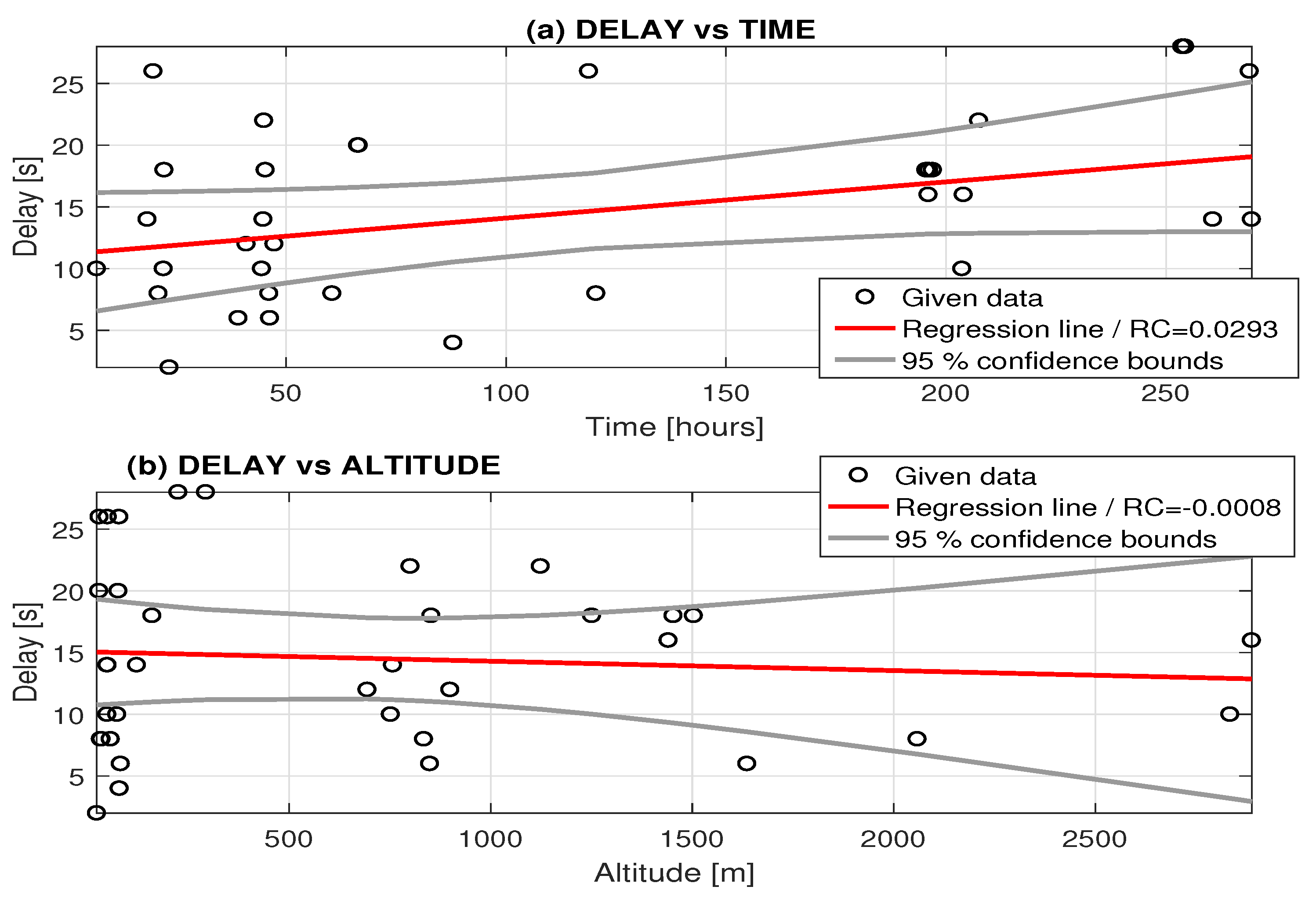
  • detection of relations between individual signals;
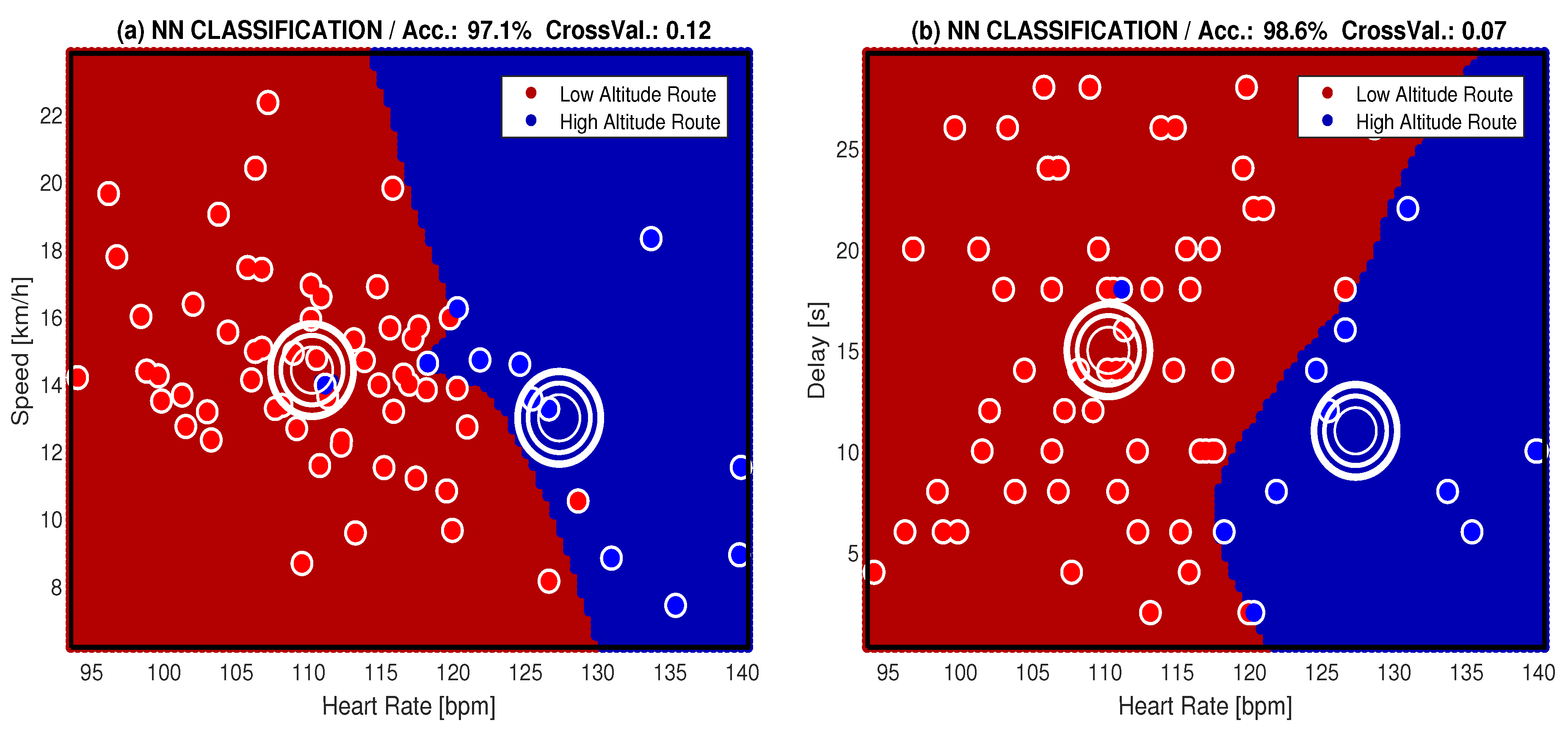
  • classification of selected segment features and evaluation of the accuracy of the classification, together with cross-validation of the model;
  • evaluation of the results from a biomedical point of view.
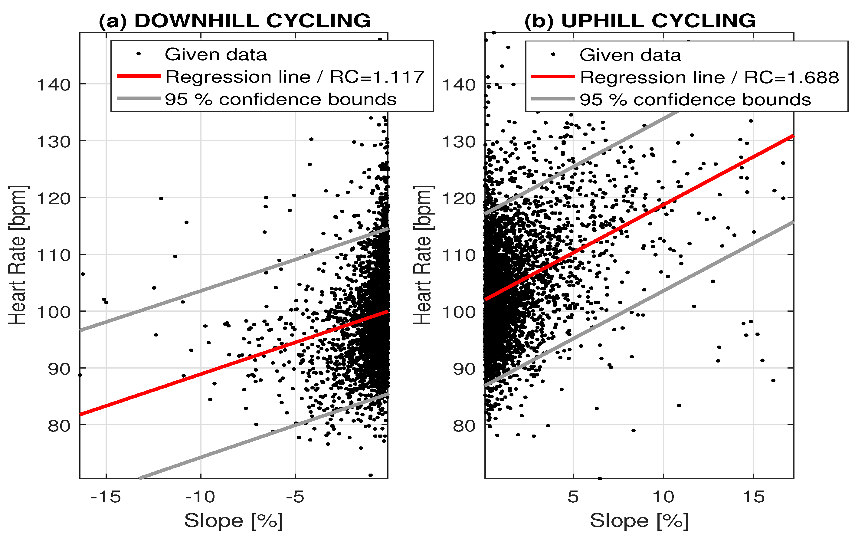
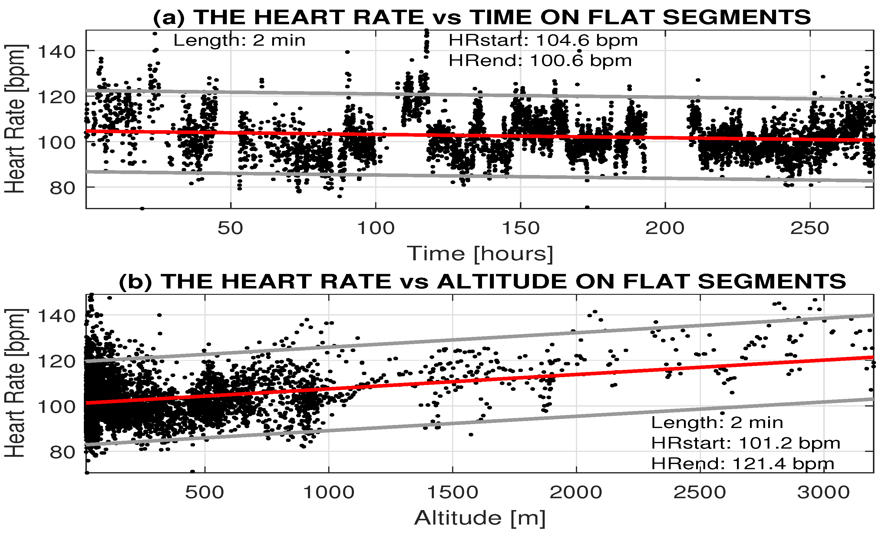
The preprocessing stage included the interconnection of all records of the cycling segments, the removal of gross observational errors, and the removal of cycling breaks. The following signal de-noising by a low-pass finite impulse response (FIR) filter was then used for the rejection of the undesirable components of each signal { x ( m ) } m = 1 M using
y ( n ) = k = 0 R 1 b ( k ) x ( n k )
for the selected filter order R = 30 and the cutoff frequency estimated from the spectral components of the individual signals. The next resampling was used to evaluate the multichannel signals of the selected constant sampling frequency f s = 0.5 Hz using spline interpolation in this stage.
The proposed method assumes the segmentation of the given signals into N-sample long segments, and their analysis. The relations between the corresponding data segments were estimated with the cross-covariance function
C x y ( k ) = 1 N i = 1 N ( x ( i ) x ¯ ) ( y ( i k ) y ¯ )
where x ¯ and y ¯ stand for the means of the individual signals { x ( n ) } n = 1 N and { y ( n ) } n = 1 N , respectively. The cross-correlation function of the sequences for the GPS and physiological data were then evaluated by
R x y ( k ) = C x y ( k ) C x x ( 0 ) C y y ( 0 )
The relation between the recorded data sequences was evaluated by estimating the correlation coefficient r x y = R x y ( 0 ) . The delay between individual signals was estimated by the cross-correlation function and its maximum value shift.
To define the relations between the corresponding segment features, the correlation coefficients were evaluated, and the 95% confidence bounds related to the regression lines were estimated.
Selected segment features were classified by the neural network (NN) [29,32], support vector machine (SVM) [33], and the k-nearest neighbour methods [34] with the evaluation of class boundaries and cross-validation by the leave-one-out method.
Cycling segment features formed the corresponding column of the pattern matrix P R , Q , as specified in Figure 4. For each cycling segment, three features forming a column vector were evaluated: the heart rate, speed, and the delay of the heart rate change after the change of the gradient altitude. This pattern matrix was then used for classification by the two-layer neural network evaluating values
A 1 S 1 , Q = F 1 ( N 1 ) , A 2 S 2 , Q = F 2 ( N 2 )
forming outputs of neural network layers where
N 1 = W 1 S 1 , R P R , Q + b 1 S 1 , 1 o n e s ( 1 , Q ) ,
N 2 = W 2 S 2 , S 1 A 1 S 1 , Q + b 2 S 2 , 1 o n e s ( 1 , S 1 )
define arguments of selected transfer functions F 1 , F 2 . An associated matrix of target values T S 2 , Q was defined by class { c ( k ) } k = 1 S 2 . One of two classes was associated with each feature vector for the cycling expedition analysis: c 1 —mean altitude less than 1500 m and c 2 —mean altitude greater than 1500 m.
Network coefficients included matrix W 1 S 1 , R of S 1 elements of the first layer with associated vector b 1 S 1 , 1 and matrix W 2 S 2 , S 1 of S 2 elements of the second layer with associated vector b 2 S 2 , 1 . The neural network included the sigmoidal transfer function F 1 in the first layer and the probabilistic softmax transfer function F 2 in the second layer [23]. Results of the output layer based on the Bayes’ theorem using function
F 2 ( N 2 ) = e x p ( N 2 ) s u m ( e x p ( N 2 ) )
provide the probabilities of each class. The number S 2 of output elements corresponds to the number of classes { c ( k ) } k = 1 S 2 . Results for R = 2 pattern values (heart rate and delay) and their classification into two classes are presented in Figure 4 and the grid of 50 by 50 elements. Owing to normalization, the sum of corresponding grid values is equal to one.

3. Results

Figure 5 presents the analysis of the changes in the heart rate related to altitude gradients along the cycling route in segments of 10 min divided into downhill and uphill cycling, with regression coefficients 1.117 and 1.688, respectively. The method was based on a correlation analysis [19] within the selected segments.
The analysis of the heart rate on flat data segments is presented in Figure 6 for two-minute data windows. Figure 6a presents the decrease of the mean heart rate in segments below an altitude of 800 m, owing to the increasing fitness level. During the 272.2 h of cycling, this mean value decreased by 4 bpm: from 104.6 to 100.6 bpm. Figure 6b presents the increase of the mean heart rate related to the mean altitude of each segment. This mean heart rate increased by 20.2 bpm from 101.2 to 121.4 bpm for altitudes ranging between 0 and 3200 m above sea level.
Figure 7a presents the delay in the change in the heart rate with the gradient of altitude for uphill cycling in 10-min segments with a correlation coefficient greater than 0.4, and its evolution over time—its increase during the cycling route being due to the (expected) increasing fitness level of the cyclist. The regression line presents its increase from 12.8 s to 16.7 s in the time range of 270 h.
In a similar way, Figure 7b presents that delay related to the altitude, with its decrease being caused by climate conditions and the decrease in air pressure with increasing altitude. The regression line presents its decrease from 15.3 s to 11.0 s for altitudes ranging between 0 and 3200 m above sea level.
Figure 8 presents the classification of selected cycling segment features by the neural network structure specified in Figure 4 into two classes defined by cycling in areas with their mean altitude (observed and recorded by the GPS system) less than 1500 m (class c 1 ) and greater than 1500 m (class c 2 ). The mean heart rate was higher for high-altitude cycling (Figure 8a), and the mean delay between the change of the heart rate to gradient altitude was lower for cycling in higher regions (Figure 8b). The summary of mean values of selected cycling features (heart rate (HR), speed, and the delay in the change in the heart rate vs. gradient of altitude) for classification into two classes ( c 1 —mean altitude less than 1500 m and c 2 —mean altitude greater than 1500 m) is presented in Table 2.
The accuracy of the neural network classification was higher than 97.1% for segments having a selected length. The comparison of the classification accuracy and cross-validation (by the leave-one-out method) of different methods (the neural network, support vector machine, and k-nearest neighbours) for classification of cycling features into two classes is presented in Table 3, with accuracy between 91.3% and 98.6%. The deviations of the measured values and evaluated features can be explained by the accuracy of the GPS system and changing climate and road conditions that can affect the cycling speed.
It is possible to expect more accurate classification from more accurate observations, more features, and more sophisticated classification methods.

4. Conclusions

This paper presented a general method of analysing GPS and heart rate data, applied to long-term multichannel cycling data. The proposed graphical user interface has been used for a correlation analysis of the heart rate related to the gradient of the altitude in data windows of downhill, flat, and uphill cycling at different altitude levels. The evaluated features were then used for the estimation of the fitness level and for the classification of selected cycling features.
The proposed method includes mathematical processing, resampling, and multichannel data analysis using general digital signal processing methods. The results obtained indicate the possibility of the use of GPS data for (i) their fusion with Google maps and visualization of the cycling tour; (ii) their correlation with heart rate data to estimate the fitness level and its monitoring; and (iii) classification with an estimation of classification boundaries.
Multimodal physiological data processing is a rapidly developing research area using data acquired by different sensors and communication systems for their transmission. The present paper is devoted to the analysis of data recorded during long-term physical activities, but it seems that a similar approach can be applied in many further areas. Visualisation and computational methods find their wide applications in assistive technologies [35], daily physical activity monitoring for the diagnosis of chronic diseases, as well as rehabilitation.
Future research will be devoted to more detailed error analysis and to deep learning methods of motion and physiological data processing. Further biomedical signals and images will also be included in the estimation of physiological features.

Supplementary Materials

The following are available online at www.mdpi.com/2076-3417/7/6/581/s1, S1: A detailed description of the cycling route, S2: a video record of a selected cycling segment, and S3: the GUI for visualization and processing of GPS and heart rate data (including all data recorded during the cycling expedition).

Acknowledgments

All real data were kindly provided by Professor Saeed Vaseghi from his cycling across the Andes in the autumn of 2016. The physiological monitoring was done at the Department of Neurology of the Faculty hospital of the Charles University in Hradec Kralove. The whole project was in support of Cancer Research UK (www.justgiving.comfundraisingsaeedvaseghi).

Author Contributions

Aleš Procházka was responsible for the mathematical and algorithmic tools allowing the data processing, Saeed Vaseghi recorded all GPS and heart rate data and contributed to their analysis, Oldřich Vyšata interpreted the acquired data and results obtained from the neurological point of view, Ondřej Ťupa contributed to the data preprocessing, and Hana Charvatová was responsible for transforming the GPS data to enable their computational processing and visualization. All authors have read and approved the final manuscript.

Conflicts of Interest

The authors declare no conflict of interest.

Abbreviations

The following abbreviations are used in this manuscript:
FIRfinite impulse response
GPSglobal positioning system
GUIgraphical user interface
HRheart rate
SVMsupport vector machine
avg.average
bpmbeats per minute
elev.elevation
km/hkm per hour

References

  1. Fister, I., Jr.; Ljubic, K.; Suganthan, P.N.; Fister, I. Computational intelligence in sports: Challenges and opportunities within a new research domain. Appl. Math. Comput. 2015, 262, 178–186. [Google Scholar] [CrossRef]
  2. Arduini, A.; Gomez-Cabrera, M.C.; Romagnoli, M. Reliability of different models to assess heart rate recovery after submaximal bicycle exercise. J. Sci. Med. Sport 2011, 14, 352–357. [Google Scholar] [CrossRef] [PubMed]
  3. Charvátová, H.; Procházka, A.; Vaseghi, S.; Vyšata, O.; Janáčová, D.; Líška, O. Physiological and GPS Data Fusion. In Proceedings of the International Workshop on Computational Intelligence for Multimedia Understanding (IWCIM), Prague, Czech Republic, 29–30 October 2015; pp. 1–4. [Google Scholar]
  4. Fasel, B.; Sporri, J.; Gilgien, M.; Boffi, G.; Chardonnens, J.; Muller, E.; Aminian, K. Three-Dimensional Body and Centre of Mass Kinematics in Alpine Ski Racing Using Differential GNSS and Inertial Sensors. Remote Sens. 2016, 8, 671. [Google Scholar] [CrossRef]
  5. Bucher, S.S.; Supej, M.; Sandbakk, O.; Holmberg, H.C. Downhill turn techniques and associated physical characteristics in cross-country skiers. Scand. J. Med. Sci. Sports 2014, 24, 708–716. [Google Scholar] [CrossRef] [PubMed]
  6. Hurst, H.T.; Swarén, M.; Hébert-Losier, K.; Ericsson, F.; Sinclair, J.; Atkins, S.; Homlberg, H.C. GPS-Based Evaluation of Activity Profiles in Elite Downhill Mountain Biking and the Influence of Course Type. J. Sci. Cycl. 2013, 2, 25–32. [Google Scholar]
  7. Formenti, D.; Trecroci, A.; Cavaggioni, L. Heart rate response to a marathon cross-country skiing race: A case study. Sport Sci. Health 2014, 11, 125–128. [Google Scholar] [CrossRef]
  8. Mekik, C.; Arslanoglu, M. Investigation on Accuracies of Real Time Kinematic GPS for GIS Applications. Remote Sens. 2009, 1, 22–35. [Google Scholar] [CrossRef]
  9. Gilgien, M.; Sporri, J.; Limpach, P.; Geiger, A.; Müller, E. The Effect of Different Global Navigation Satellite System Methods on Positioning Accuracy in Elite Alpine Skiing. Sensors 2014, 14, 18433–18453. [Google Scholar] [CrossRef] [PubMed]
  10. Erden, F.; Velipasalar, S.; Alkar, A.Z.; Cetin, A.E. Sensors in Assisted Living: A survey of signal and image processing methods. IEEE Signal Process. Mag. 2016, 33, 36–44. [Google Scholar] [CrossRef]
  11. Ahmad, F.; Cetin, A.E.; Ho, K.C.; Nelson, J. Signal Processing for Assisted Living: Developments and Open Problems. IEEE Signal Process. Mag. 2016, 33, 25–26. [Google Scholar] [CrossRef]
  12. Bang, Y.; Kim, J.; Yu, K. An Improved Map-Matching Technique Based on the Fréchet Distance Approach for Pedestrian Navigation Services. Sensors 2016, 16, 1768. [Google Scholar] [CrossRef] [PubMed]
  13. Maddison, R.; Ni Mhurchu, C.; Cavaggioni, L. Global Positioning System: A new opportunity in physical acivity measurement. Int. J. Behav. Nutr. Phys. Act. 2009, 6, 73. [Google Scholar] [CrossRef] [PubMed]
  14. Damani, A.; Shah, H.; Shah, K.; Vala, M. Global Positioning System for Object Tracking. Int. J. Comput. Appl. 2015, 109, 40–45. [Google Scholar] [CrossRef]
  15. Drawil, N.M.; Amar, H.M.; Basir, O.A. GPS localization accuracy classification: A context-based approach. IEEE Trans. Intell. Transp. Syst. 2013, 14, 262–273. [Google Scholar] [CrossRef]
  16. Schmid, A. Positioning Accuracy Improvement with Differential Correlation. IEEE J. Sel. Top. Signal Process. 2009, 3, 587–598. [Google Scholar] [CrossRef]
  17. Wang, H.; Ou, J.; Yuan, Y. Strategy of Data Processing for GPS Rover and Reference Receivers Using Different Sampling Rates. IEEE Trans. Geosci. Remote Sens. 2011, 49, 1144–1149. [Google Scholar] [CrossRef]
  18. Whyte, G.P.; George, K.; Shave, R.; Middleton, N.; Nevill, A.M. Training Induced Changes in Maximum Heart Rate. Int. J. Sports Med. 2008, 29, 129–133. [Google Scholar] [CrossRef] [PubMed]
  19. Procházka, A.; Vaseghi, S.; Yadollahi, M.; Ťupa, O.; Mareš, J.; Vyšata, O. Remote Physiological and GPS Data Processing in Evaluation of Physical Activities. Med. Biol. Eng. Comput. 2013, 52, 301–308. [Google Scholar] [CrossRef] [PubMed]
  20. Charvátová, H.; Procházka, A.; Vaseghi, S.; Vyšata, O.; Vališ, M. GPS-based Analysis of Physical Activities Using Positioning and Heart Rate Cycling Data. Signal Image Video Process. 2016, 1–8. [Google Scholar] [CrossRef]
  21. Procházka, A.; Vyšata, O.; Vališ, M.; Ťupa, O.; Schatz, M.; Mařík, V. Use of Image and Depth Sensors of the Microsoft Kinect for the Detection of Gait Disorders. Neural Comput. Appl. 2015, 26, 1621–1629. [Google Scholar] [CrossRef]
  22. Muro-de-la-Herran, A.; Garcia-Zapirain, B.; Mendez-Zorrilla, A. Gait Analysis Methods: An Overview of Wearable and Non-Wearable Systems, Highlighting Clinical Applications. Sensors 2014, 14, 3362–3394. [Google Scholar] [CrossRef] [PubMed]
  23. Procházka, A.; Vyšata, O.; Vališ, M.; Ťupa, O.; Schatz, M.; Mařík, V. Bayesian Classification and Analysis of Gait Disorders Using Image and Depth Sensors of Microsoft Kinect. Digit. Signal Process. 2015, 47, 169–177. [Google Scholar] [CrossRef]
  24. Shi, G.; Wang, Y.; Li, S. Human Motion Capture System and its Sensor Analysis. Sens. Transducers 2014, 172, 206–212. [Google Scholar]
  25. Ťupa, O.; Procházka, A.; Vyšata, O.; Schatz, M.; Mareš, J.; Vališ, M.; Mařík, V. Motion tracking and gait feature estimation for recognising Parkinson’s disease using MS Kinect. Biomed. Eng. Online 2015, 14, 97. [Google Scholar] [CrossRef] [PubMed]
  26. Hostalkova, E.; Vysata, O.; Prochazka, A. Multi-dimensional biomedical image de-noising using Haar transform. In Proceedings of the 15th International Conference on Digital Signal Processing, Cardiff, UK, 1–4 July 2007; Sanei, S., Chambers, J., Eds.; Cardifff University: Cardiff, UK, 2007; pp. 175–178. [Google Scholar]
  27. Jerhotová, E.; Švihlík, J.; Procházka, A. Biomedical Image Volumes Denoising via the Wavelet Transform. In Applied Biomedical Engineering; Gargiulo, G.D., McEwan, A., Eds.; INTECH: Rijeka, Croatia, 2011; pp. 435–458. [Google Scholar]
  28. Vaseghi, S. Advanced Signal Processing and Digital Noise Reduction; Wiley & Teubner: West Sussex, UK, 2000. [Google Scholar]
  29. Bishop, C.M. Pattern Recognition and Machine Learning; Springer: Cambridge, UK, 2006. [Google Scholar]
  30. Procházka, A.; Vyšata, O.; Ťupa, O.; Mareš, J.; Vališ, M. Discrimination of Axonal Neuropathy Using Sensitivity and Specificity Statistical Measures. Neural Comput. Appl. 2014, 25, 1349–1358. [Google Scholar] [CrossRef]
  31. Lin, I.-C.; Peng, J.-Y.; Lin, C.-C.; Tsai, M.-H. Adaptive Motion Data Representation with Repeated Motion Analysis. IEEE Trans. Vis. Comput. Graph. 2011, 17, 527–538. [Google Scholar]
  32. Theodoridis, S.; Koutroumbas, K. Pattern Recognition; Academic Press: Cambridge, MA, USA, 2009. [Google Scholar]
  33. Bouboulis, P.; Theodoridis, S.; Mavroforakis, C.; Evaggelatou-Dalla, L. Complex Support Vector Machines for Regression and Quaternary Classification. IEEE Trans. Neural Netw. Learn. Syst. 2015, 26, 1260–1274. [Google Scholar] [CrossRef] [PubMed]
  34. Kataria, A.; Singh, M.D. A Review of Data Classification Using k-Nearest Neighbour Algorithm. Int. J. Emerg. Technol. Adv. Eng. 2013, 3, 354–360. [Google Scholar]
  35. Chen, H.; Wang, G.; Xue, J.H.; He, L. A novel hierarchical framework for human action recognition. Pattern Recognit. 2016, 55, 148–159. [Google Scholar] [CrossRef]
Figure 1. The use of the proposed graphical user interface for the analysis of a data segment 183 km long and a window beginning 4255 km after the expedition’s starting point, showing its position on the map and the signals recorded in this selected time/length region, along with some fundamental features of the segment.
Applsci 07 00581 g001
Figure 2. Detailed part of the cycling expedition across the Andes mountains (10 km long), recorded for 28 min of downhill cycling with an average speed of 22 km/h.
Applsci 07 00581 g002
Figure 3. Multimodal data recorded during the whole cycling route (5694-km long) across the Andes mountains, presenting (a) GPS global and detailed altitude data; and (b) heart rate data with cycling segment specifications.
Applsci 07 00581 g003
Figure 4. The diagram of multimodal cycling data processing and signal segments classification presenting outputs of the first and the second elements of the neural network (NN) output for classification into S 2 = 2 classes.
Applsci 07 00581 g004
Figure 5. The evolution of the heart rate related to the slope in selected 10-min segments: (a) downhill cycling; (b) uphill cycling.
Applsci 07 00581 g005
Figure 6. The evolution of the heart rate related to time in selected flat two-minute segments: (a) decrease of the heart rate in segments below an altitude of 800 m owing to the increasing fitness; (b) the increase of the mean heart rate related to altitude.
Applsci 07 00581 g006
Figure 7. The delay of the change in the heart rate with gradient of altitude for uphill cycling in 10-min segments and correlation coefficients larger than 0.4, presenting its evolution (a) in time, owing to the increasing fitness level; and (b) with the altitude, owing to climate conditions.
Applsci 07 00581 g007
Figure 8. Neural networks (NN) classification of 10-min segments for uphill cycling into two separate classes ( c 1 —mean altitude less than 1500 m and c 2 —mean altitude greater than 1500 m) and the mean heart rate related to (a) the mean speed and (b) the delay in the change in the heart rate vs. gradient of altitude presenting centers of gravity of class features.
Applsci 07 00581 g008
Table 1. Specification of the cycling expedition across the Andes mountains.
Cycling route length5694 km
Total cycling time272.2 h
Average speed (km/h)20.9 km/h
Number of cycling segments48
Average segment length118.6 km
Table 2. Comparison of means and standard deviations (STD) of selected cycling features (heart rate (HR), speed, and the delay in the change in the heart rate vs. gradient of altitude) for classification into two classes ( c 1 —mean altitude less than 1500 m and c 2 —mean altitude greater than 1500 m).
FeatureClass 1Class 2
MeanSTDMeanSTD
HR (bpm)110.37.6127.48.9
Speed (km/h)14.42.813.03.2
Delay [s]15.07.511.05.6
Table 3. Comparison of accuracy and cross-validation for classification of two cycling features into two classes ( c 1 —mean altitude less than 1500 m and c 2 —mean altitude greater than 1500 m) by neural network (NN), support vector machine (SVM), and k-nearest neighbours (5-NN and 7-NN) methods.
Speed vs. HRDelay vs. HR
MethodAccuracyCrossValAccuracyCrossVal
(%) (%)
NN97.10.1298.60.07
SVM95.70.1292.80.10
5-NN92.80.1092.80.10
7-NN92.80.0991.30.13

