Survey on Modelling and Techniques for Friction Estimation in Automotive Brakes
by
 , ,
, ,
Vincenzo Ricciardi
1,* ,
,
Klaus Augsburg
1,
Sebastian Gramstat
2,
Viktor Schreiber
1 and
Valentin Ivanov
1
1
Automotive Engineering Group, Technische Universität Ilmenau, 98693 Ilmenau, Germany
2
Development Foundation Brake, AUDI AG I/EF-51, 85045 Inglostadt, Germany
*
Author to whom correspondence should be addressed.
Appl. Sci. 2017, 7(9), 873; https://doi.org/10.3390/app7090873
Submission received: 28 June 2017
/
Revised: 7 August 2017
/
Accepted: 21 August 2017
/
Published: 25 August 2017
(This article belongs to the Section Mechanical Engineering)
Abstract
:The increased use of disc brakes in passenger cars has led the research world to focus on the prediction of brake performance and wear under different working conditions. A proper model of the brake linings’ coefficient of friction (BLCF) is important to monitor the brake operation and increase the performance of control systems such as ABS, TC and ESP by supplying an accurate estimate of the brake torque. The literature of the last decades is replete with semi-empirical and analytical friction models whose derivation comes from significant research that has been conducted into the direction of friction modelling of pin-disc couplings. On the contrary, just a few models have been developed and used for the prediction of the automotive BLCF without obtaining satisfactory results. The present work aims at collecting the current state of art of the estimation techniques for the BLCF, with special attention to the models for automotive brakes. Moreover, the work proposes a classification of the several existing approaches and discusses the relative pro and cons. Finally, based on evidence of the limitations of the model-based approach and the potentialities of the neural networks, the authors propose a new state observer for BLCF estimation as a promising solution among the supporting tools of the control engineering.
1. Introduction
1.1. General Remarks
The tightening up of regulations on driving safety [1] and emissions has pushed researchers to develop outperforming solutions aimed at reducing environmental impact and energy consumption. It is evident that, in accordance with this trend, in a few years the non-exhaust emissions from vehicles will also be regulated. Indeed, a review of the Institute for Energy and Transport of the European Commission reports PM10 brake wear emission rates up to 8.8 mg/km and PM2.5 rates up to 5.5 mg/km for passenger cars [2]. Bearing in mind that the last regulations for diesel engines set a limit of 5 mg/km for PM10 from exhaust, it is clear that friction brakes and tires are nowadays considered the main emitters of micro- and nanoparticles in road vehicles next to internal combustion engines [3]. Therefore, wear and emissions estimations, along with brake enhancement, require the development of a reliable model of brake linings’ coefficient of friction (BLCF).
Unfortunately, analytical representation of the pad–disc tribological contact is challenging, which in turn influences the brake operation by varying the BLCF: fading [4,5]; bedding [6]; hysteresis against the pressure [7]; hysteresis against the speed [8], wear [9,10], and aging [6]; and variation in the environmental conditions [11]. The behaviour of a pad–disc coupling is also dependent on the chemical composition and mechanical properties of each component [12].
In addition to the abovementioned, there are also other phenomena that must be taken into consideration when studying the brake tribology: (i) thermally induced deformation of the brake pad due to non-uniform temperature distribution; (ii) non-uniform pressure distribution over the pad surface owing to calliper deformation, especially for low-pressure applications; (iii) the presence of residual grinding torque even without brake application; (iv) chemical contamination processes of the contact plateaus owing to oxidation or inclusion of re-suspended road dust particles. It therefore seems clear that when creating a model capable of predicting the real BLCF by taking into account the abovementioned phenomena, is important to monitor the brake operation and optimize its actuation.
A thorough experimental analysis is still demanded in the field of optimal control of automotive brakes. Actually, just a few analytical models have been employed for modelling the BLCF in automotive brakes. The reason is that many of the proposed models are only suitable to describe the common pin–disc contact in a controlled environment [13,14,15]; therefore, they are not suitable to depict the automotive brake pad–disc interface. The latter problem involves dry sliding contact, although the pads could be unintentionally lubricated, e.g., due to rain. Most of the time the sliding occurs at high speed and high forces and consequently implies high temperatures: during hard brake manoeuvres, the kinetic energy dissipated into the brake pad can easily exceed 30 kW [6].
With reference to the pad–disc tribological contact, it is experimentally assessed that the BLCF is linked to the number of contact plateaus between the pad and the disc [6,16], constituting approximately 20% of the pad area. The contact plateaus can grow or decay in relation to processes that involve agglomeration and compaction of the wear debris around the nucleation sites [17]. These phenomena are influenced by the contact temperature, the humidity [18] and the local pressure [19]. Therefore, in relation to the plateaus in birth–growth–destruction dynamics [17], the BLCF can range between 0.3 and 0.6 [12,20], with peaks up to 0.8 and down to 0.1 [4,17]. Among the recorded instances in the literature, it is also possible to encounter extreme values of the BLCF with special specimens, e.g.,: a lower value of 0.04 for polyamide linings reinforced with glass fibres and an upper value of 2.0 for polyamide/steel linings [21].
Previous reviews that have attempted to survey friction laws for “various mechanical objects” [22,23] partially cover the topic of BLCF estimation [24] without providing an insight into automotive brakes. The present work aims at offering a complete and thorough starting point for everyone who wants to grapple with the topic of BLCF estimation in automotive brakes. The interested reader is provided with an overview of the phenomena occurring in pad–disc contact that cause a remarkable variation in the BLCF. An understanding of friction phenomena is necessary for control engineers, proving the interest of this community in designing control laws for friction compensation [25] and wear reduction. Eventually, the present work also aims at evidencing the possibility of applying the state observation technique for the estimation of the BLCF.
1.2. Motivations
It is worth noting that in recent decades phenomenological and empirical models, along with experimental techniques, have evolved compared to the first studies of Coulomb more than 200 years ago. Friction modelling has undergone consistent development, mainly in applications involving small displacements and velocities where the static friction and pre-sliding displacement play crucial roles [26]. As an example, friction modelling has been a matter of study for control engineering due to the necessity of developing estimators to compensate for the friction forces of the electric machines for high-precision applications (e.g., haptic applications) [26,27]. Indeed, the modelling and compensation of friction dynamics is a topic of interest for the machining and assembly industry, where high-accuracy positioning systems are much in demand.
The main task of the BLCF model is to correlate the friction coefficient to system inputs such as the brake pressure, and to system states such as the brake temperature and disc speed. Friction is a very complex force to render; it depends on a large variety of parameters such as sliding speed [28], sliding acceleration [29], temperature, normal load [30], environment conditions [18,31], surface finishing [32] and chemical composition [12]. With the aim of identifying a model capable of predicting the real BLCF, it is necessary to understand the phenomena affecting the brake operation. The performance of this task would represent an important advancement in the field of driver assistance systems for the enhancement of innovative functions such as conventional and regenerative brake blending in electric vehicles [33] and the improvement of well-known features such as wear and NVH (noise–vibration–harshness) [34]. A model capable of predicting the value of the BLCF could be useful to improve driving safety during emergency braking, and to enhance brake actuation during service braking.
2. Techniques for the Estimation of BLCF in Automotive Disc Brakes
2.1. General Remarks
In this section, the work concentrates on research into a tool capable of predicting the actual BLCF in automotive brakes. As repeatedly stated, the requested tool is important to monitor the brake operation and its actuation for safety and environmental purposes.
During the last decades, ever more sophisticated models have been developed.
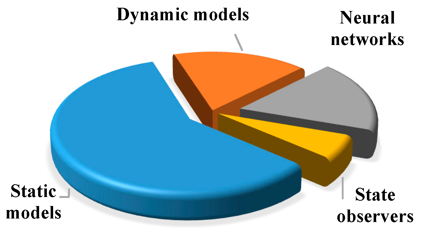
As reported in Figure 1, the techniques in the literature range among:
- static and dynamic models, which require an ad hoc parameter calibration against the specific plant;
- neural networks, which demand an accurate design of experiments for the learning and training process;
- state observers, which give an estimation based on information provided by the vehicle sensors without the need to accurately model the phenomena affecting the tribological contact.
In the following, the text highlights limitations and dwells on a comparative analysis among the existing techniques. First, studies regarding the classical model-based approach are surveyed. Among these, Ostermeyer’s dynamic model [17] is acknowledged as the most advanced model among the brake community. Hereunto, the paper provides an assessment of the latter, which proves to be unsuitable for on-board applications. In addition, the cellular automata method is featured as a supporting tool to the classical model-based approach for the depiction of frictional and wear behaviour in the contact zone. Thereafter, artificial neural networks are presented as an effective technique to handle nonlinear dynamic modelling in the place of phenomenological regression models, whose application would be awkward and cumbersome. In conclusion, a new methodology based on the state observation technique will be herein proposed as an innovative solution for online estimation of the BLCF. This latter is expected as a promising solution since it uses measurements coming directly from the vehicle sensors by avoiding an analytical description of the brake phenomenology and does not require the implementation of models that cause a high computational burden, such as temperature distribution models. The observer results are compared to a reference profile generated through the vehicle dynamics simulator IPG CarMaker.
2.2. Static and Dynamic Model-Based Approaches for the Estimation of BLCF
In many studies, the calliper pressure has been used to calculate the brake torque, assuming a constant BLCF [35]. It is clear that this assumption is not feasible when one is interested in predicting the actual BLCF since it is influenced by the operating and environmental conditions. For this reason, it is important to take into consideration the phenomena affecting the braking by applying a formulation that captures environment and state dependences.
Referring to the state of the art, it is noticeable that a wealth of different models have been implemented for the prediction and estimation of friction properties in automotive brakes under determined working conditions. In [36] an alternative formulation based on the switching between the stick and slip motion is proposed by considering a rate-dependent dumping term for the Stribeck effect and an elastic term for the pre-sliding modelling [37,38]. In [39], a simple quadratic model in the velocity state, based on experimental tests, is used. In [40], an analytical formulation considering only the friction dependence against the speed is proposed. A very simple analytical formulation based on steady-state experimental tests that correlate the pressure, speed and temperature dependences to the friction and wear is assessed in [41]. In [42] an alternative formulation is put forth that, in addition to the sliding speed, involves thermal effects due to the increase in temperature of the friction materials. In [43] a simplified static LuGre model is used under the assumption that the friction dynamics is considerably faster than the other phenomena involving the vehicle dynamics and therefore negligible for simulation purposes: the friction dynamics is neglected by substituting the state with constants and the formula is augmented with a temperature-dependent term. A dynamic LuGre model is employed in [44] to determine the friction force between the disc and the pad. In addition, the authors in [45] propose a novel static formulation as a function of the brake temperature, brake pressure and braking speed. Experimental data collected from the pin–disc test rig are used to calibrate the model. Finally, in [46], a scaled inertia brake dynamometer is used to investigate the frictional characteristics of three lining materials, based on low-metallic, semi-metallic and non-asbestos inorganic composition, respectively. A dynamic model whose parameters depend on the initial load conditions is developed to measure the frictional dependence against the load, temperature and speed.
Unfortunately, the majority of BLCF models have not been subjected to experimental assessment but only to simulation tasks. The listed formulations are not capable of depicting the hysteresis behaviour of BLCF against varying speed and pressure. Hence, they do not constitute reliable solutions for BLCF estimation in automotive brakes and cannot be used for real applications. Moreover, most of the abovementioned models do not account for the combination of thermal and mechanical behaviour of the contact since the temperature does not appear as an influencing variable of the BLCF. It is well known that the extreme temperatures reached during the braking actions have a strong impact on the brake performance and can bring about undesired phenomena such as the fading effect, even for metal pads [4,5]. The FEM technique has been widely applied for temperature distribution estimation and squeal analysis in disc brakes [47,48]. However, owing to the high computational burden, it is not possible to use this approach for an online estimation of the brake temperature. For this reason, it is not feasible to use the finite element method, along with a friction model, for prediction purposes. The results presented in the literature refer to off-line simulation analysis, wherein, wrongly, BLCF is assumed to have a constant value [49,50]. Regardless, in the following rows, two simple models that try to capture the temperature influence on the brake effectiveness are reported.
In [51], Chichinadze introduces a static model that takes into account the temperature dependence of the BLCF for different pad compositions. It is possible to further understand the capabilities of this approach by explicating the proposed formulation. The dependence of BLCF on the temperature , in accordance with the method proposed in [51], has the form:
The coefficients and are defined experimentally and depend on the pad chemical composition. The main drawback of this model is that it does not account for the static friction, giving no analytical formulation for the stick regime, and does not consider the dynamics of BLCF itself. Above all, this model does not reproduce the Stribeck effect and consequently the hysteresis against the speed.
In [17], Ostermeyer proposes a dynamic model for the prediction of BLCF based on two differential equations: the former estimates BLCF; the latter represents the temperature state. This dynamic model tries to capture the dynamical behaviour of BLCF and its dependence on temperature, thus explaining the fading effect of the brake system. The frame of the model rests on the assumption that BLCF is the result of the equilibrium between the flow of birth and death of contact patches.
It is worth noticing that the destruction of the plateaus depends on the wear of the neighbouring plateaus, their temperature and the local mechanical stress. The described process is responsible for the equilibrium of the patch flow and thereby determines the friction and wear behaviour of the contact. The patches are responsible for the transformation of the kinetic energy into friction. In particular, both the number and size of the contact patches are tied to the heat and wear phenomena: indeed, the wear causes a particle flow that increases the size of the contact patches; the heat modulates the wear and thus the destruction of the contact patches [17]. Heat and wear are in turn induced by the sliding resistance. A schematic representation of this process is reported in Figure 2.
Along with the friction modelling, this approach also embeds the wear effect on the brake dynamics; a reduction of the pad thickness affects the temperature space distribution and, above all, the wear is responsible for the destruction of the contact plateaus. This model is able to capture the fading effect thanks to the inclusion of the temperature dependence, but, as shown later, is unable to render the hysteresis phenomenon against the sliding speed and the pressure. The typical formulation dwells on the following set of differential equations:
The first equation depicts the dynamics of the BLCF ; the latter represents the dynamics of the brake temperature in the contact region. The group represents the magnitude of the combination between the calliper normal load and the brake disc speed; are constant parameters linked to the pad chemical composition. In particular, the parameter is responsible for the growing behaviour of the patches against the temperature and thus of the increase of the BLCF; is instead responsible for the destructive behaviour of the mechanical grinding action; the parameter is linked to the real area of contact patches. The term in parentheses in Equation (2) describes the destructive effect linked to the friction power and the extent of the patches area, supposedly proportional to BLCF. Equation (3) comes from the heat balance equation including the convective exchange with the environment, neglecting the radiation phenomenon, and considering the generation term due to the friction. The parameter rules the part of friction power transformed into heat.
In conclusion, it has been illustrated that the tribological disc–pad contact also includes the heat transfer, which is a complex phenomenon to describe and implies high computational burden. As already stated, an analytical description of the heat transfer phenomenon is difficult and not suitable for implementation in control strategies. For this reason, two simple models, static and dynamic, that encompass the temperature effect on the BLCF, have been presented.
Assessment of Ostermeyer’s Model
In the present subsection, an assessment of Ostermeyer’s model is featured, consisting in its identification and validation against the experimental data acquired on the brake dynamometer with a climatic chamber at the Technische Unversität Ilmenau. A general overview of the test rig is reported in Figure 3. This dynamometric brake stand is used to test the performance and NVH characteristics of brake systems under various and controlled conditions. The brake dynamometer is controlled through the manufacturer’s software, which ensures a seamless control of the system actuators. The compressed air hydraulic actuator increases the pressure up to 21 MPa within the master cylinder. The system is equipped with a flow meter of the brake fluid and a pressure sensor that measures the actual pressure on the calliper. The brake torque is measured through a sensor positioned inside the inertial hub and corresponds to the output torque. The dynamometer allows a maximum operating regime of 2500 rpm and features a peak power of 186 kW and maximum torque of 5000 Nm. The test was conducted under the “drag mode” in order to ensure a constant sliding speed during oscillating input brake pressure.
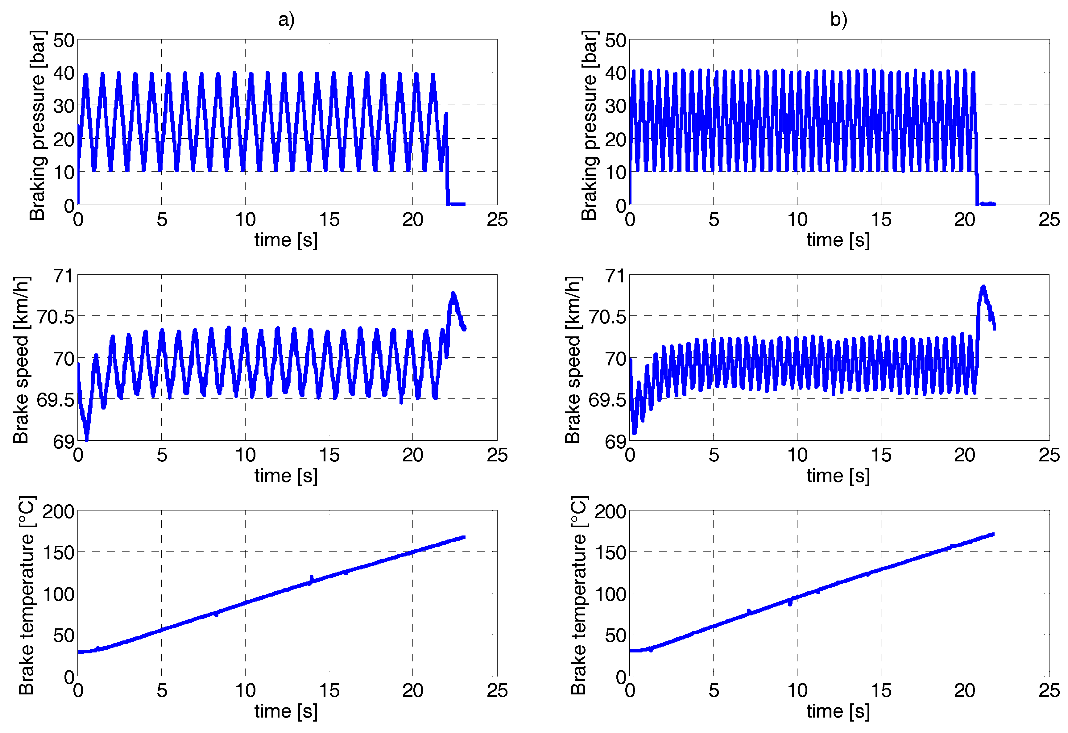
The brake pressure complies with a saw tooth signal with fixed frequency; therefore, the term in Equation (3) varies proportionally to the pressure law. In particular, the second test (Figure 4b) features an input frequency double that of the first one (Figure 4a). Moreover, during the test, the brake undergoes increasing temperature, a condition that affects the brake performance. In the first instance, the dynamic model in Equations (2) and (3) has been identified against the first set of experimental data and, in the second instance, validated against the second dataset, Figure 4. These manoeuvers emulate an extreme scenario of brake actuation that occurs in case of prolonged ABS intervention. For the model parameters identification, a minimization algorithm based on the Newton’s method has been applied [52]. Within the optimization procedure, Equations (2) and (3) are computed for the whole time providing that is set to zero when no pressure is applied on the callipers.
In the following rows, the validation and identification results will be analysed by comparing the experimental and the model predicted braking torque. This latter can be easily calculated in compliance with the following:
where is the braking torque, is the BLCF computed from Equation (2), represents the actuated brake pressure, and and are geometric factors, namely the calliper area and the radial position of the brake calliper application point. Figure 5a displays the outcome of the identification process conducted against the first dataset. This fitting was achieved by solving an optimization problem whose input variables are the parameters of the model, . The identification procedure led to the following model parametrization: . As shown in Figure 5a, it is noticeable that in the presence of increasing temperature the simulated profile remains aligned to the experimental reference. This result was anticipated since the model under discussion takes into account the friction dependence against the temperature.
In Figure 5b, the validation test against the second dataset is instead reported. Although a lack of accuracy is evident corresponding to the low temperature values (the first five seconds), the model exhibits good overall capability in predicting the braking toque, even for varied brake actuation frequency. Thanks to the inclusion of a temperature-dependent term in the analytical formulation, the model remains close to the experimental profile.
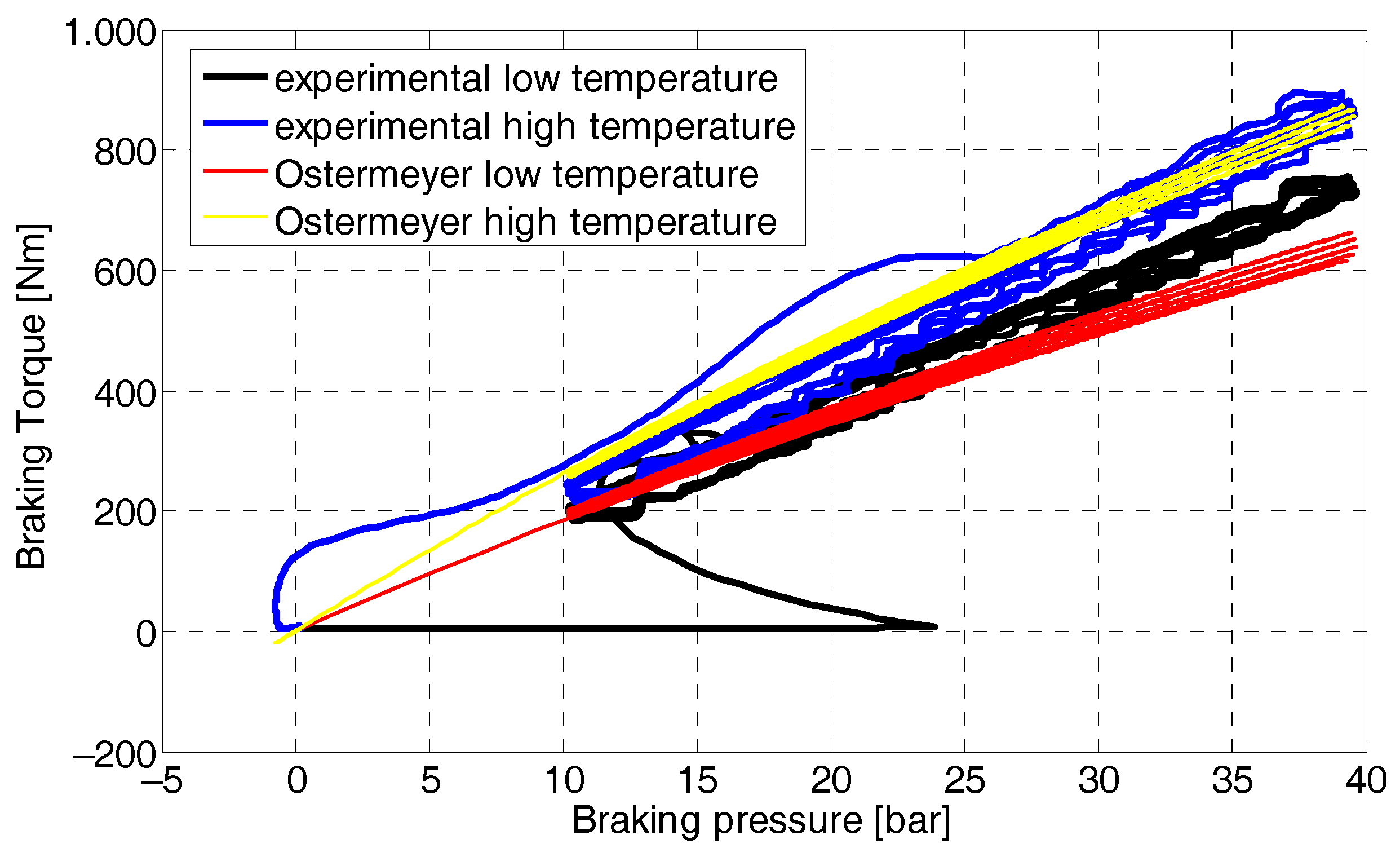
In Figure 6, the resulting braking torque has been plotted against the actuated pressure in order to examine the model’s ability to reproduce the hysteresis effect. It appears clear that the model under analysis does not capture the hysteresis behaviour of the BLCF against the pressure oscillations.
This issue has been addressed in [7], wherein the Ostermeyer’s model is used in conjunction with the Bouc–Wen model in order to capture the hysteresis dynamics against varying pressure. This solution overcomes the evident limitation of Equation (2) so that the negative influence of the brake hysteresis on the vehicle dynamics can be accounted for. The work in [7] eventually concludes that the model is not capable of capturing the fast dynamics of BLCF and the relative error between the real and the estimated BLCF can reach values up to 15–20%.
In conclusion, the dynamic model [17] assessed here is not suitable for online prediction of BLCF. It does not reproduce the frictional hysteresis against the pressure despite its ability to render other dynamic behaviours such as the influence of the temperature on the BLCF. Nevertheless, a strong drawback of this model is the requirement of an ad hoc parametrization depending on the specific plant.
The following subsection puts forth cellular automata as an effective tool to describe the friction and wear on the nanometre scale. It is worth remarking that direct observation of the friction layer during a brake application is not possible. Hereunto, the cellular automata provide a detailed insight into the dynamics of the contact interface and represent a supporting tool for model-based approaches.
2.3. An Extension of the Model-Based Approach—The Cellular Automata Model
The cellular automata were formerly introduced by Stanislaw Ulam in the 1940s but their application as a generic calculation technique was formulated by John von Neumann [53]. Their field of application ranges among problems of biology, transport and physics but their use in tribological systems is relatively recent [54]. As frequently mentioned, the tribological behaviour of the system is determined by the growth and destruction of characteristic hard structures on a mesoscopic scale [17]. Hereto, the cellular automata have been revealed as an effective tool to render the patch life cycle, consisting of the growth and destruction phase or alternatively in the growth and detachment process with the ability to depict the particle flow. The integration of the cellular automata model with a friction law in macroscopic models, such as Ostermeyer’s model, allows for tightening the gap between the surface topography dynamics and the macroscopic phenomena. The actual aim of the cellular automata is to obtain a guess at the frictional behaviour at the pad–disc contact with relation to the patches’ dynamics.
Cellular automata are characterized by the following elements: (i) a regular lattice, whose elements are the cells, represents the spatial discretization of the space; (ii) a finite set of inner variables for each cell; (iii) a finite set of rules and functional relations among the neighbouring cells that leads the cellular development; (iv) a transition function concerning the cell neighbourhood and updating the inner variables at each time increment.
The lattice is constituted by the spatial discretization of the pad–disc contact under the form of cells. The patch size in pad–disc contact is approximately some hundred microns, as experimentally assessed. That is why it is necessary to choose a lattice so that the cellular size is sufficiently small compared to the characteristic patch dimensions. For instance, the authors in [54,55] define each cell as 10 µm × 10 µm in order to depict the patch growth in detail (Figure 7).
In accordance with many authors, each cell contains a set of four inner variables. The first inner variable is the status of a cell that can be “patch” or “not patch” depending on whether the cell belongs to a patch or not. The second variable is the friction power of a cell caused by the local friction force and the relative velocity of the cell. For each cell, the temperature is also computed as the third inner variable, by considering the mutual interaction among neighbouring cells. Finally, the particle density stands as an index for the wear volume: the more the generated particles agglomerate, the more the density increases.
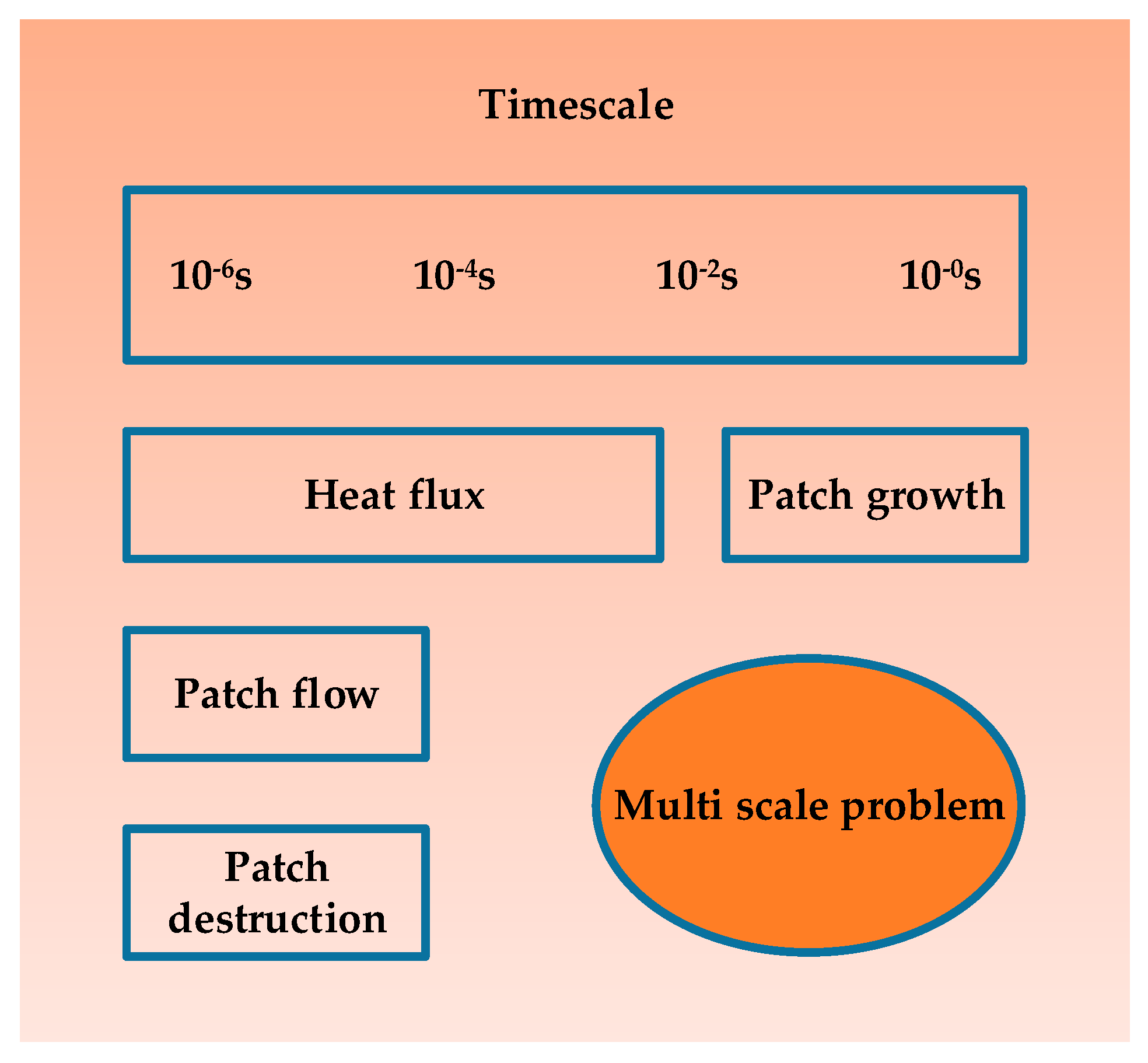
It is worth noting that the four properties are tied to each other by means of rules. The interactions among the cells’ inner variables occur on different timescales, therefore every single process has to be simulated against different time steps, as shown in Figure 8. For instance, the phenomena of patch destruction and flow occur on a time scale of µs; instead, the processes of patch birth and growth occur on a time scale ranging between and [54]. This means that in the timescale of µs the heat flux and the wear particle stream must be computed, whereas these terms can be assumed to have stationary values in the timescale of seconds. This explains why it is necessary to separate each phenomenon and integrate it with a sample time aimed at minimizing the computational burden.
It is expected that there exist mutual influences among the abovementioned variables and each interaction withstands a rule constituting the cellular automata algorithm. Several authors introduce a particular set or rules derived from physical laws and experimental assessments, which describe the interactions between the patches, friction coefficient, wear and temperature. Although they have diverse purposes, each work puts forth the potentialities of the cellular automata employed to analyse the disc brake interface behaviour. For a better comprehension of the transition functions among the cells, see [55].
The authors of [55] believe that a model that encompasses the dynamic on a mesoscopic scale is a promising tool to provide a qualitative description of the patch life cycle, which is responsible for the variation in the surface topography. In other words, it is a suitable approach to obtain insight into the pad–disc interface. The authors of [57] propose a simulating tool based on 2D cellular automata that can be used to determine the concentration of airborne wear particles generated from disc brakes. To achieve this goal, a model able to describe the physical behaviour of the contact situation in disc brakes is sought. In [56], the cellular automata model is extended to render the surface topography in three dimensions in order to comprehend the tribological behaviour under different load conditions. In [58] cellular automata are used to investigate the behaviour of the hard patches on a nanoscale length under the influence of different pad chemical compositions.
Another technique that has been recently applied in the considered tribology field is the Movable cellular automata (MCA). The concept of the MCA is based on the conventional concept of cellular automata but, in addition to the basic postulates, the elementary object is also characterized by translational and rotational degrees of freedom. This tool is suitable for the visualization of friction processes on the nanometre scale, such as topography modification, film degradation and mass mixing. In [58,59] the frictional behaviour against the local contacts in an automotive brake system has been analysed on the basis of computer simulation by means of the MCA. This technique has been applied with satisfactory results, showing a good qualitative correspondence between the model results and the experimental evidence.
The cellular automata method renders the particle flow and the interaction between the patches and the particle motion [54]. Indeed, upon reaching a patch, the particles are either deflected or agglomerated. For this reason, the wear particle density beside and in front of these regions is maximal; instead, within the wakes of the patches, the number of wear particles is rather low. As it arises from the literature, the results are stable, and thus the set of rules is consistent in each timescale. The information obtained by the cellular automata simulation on the contact surfaces’ topography could be used as an input for a macroscopic model. The choice of inner variables, rules, and boundary conditions allows for determining the tribological properties of the system. This includes the heat flux, the wear particle stream, patch growth and patch destruction. As has been explained and itemized, these processes occur on different timescales. This kind of simulation is very helpful to comprehend the particle flow on a very small scale but, due to the reduced particle sizes and time steps that cause a high computational burden, conclusions towards a global friction behaviour are not possible.
2.4. Neural Networks for BLCF Estimation
As seen previously, owing to the manifold phenomena affecting the brake operation and the awkwardness of rendering each of them, the existing analytical formulations provide unsatisfactory results. Moreover, considering that the models’ parameters must be identified over again in case of a change in the plant characteristics, it is clear that the models are unreliable for online applications. These issues led to another approach, namely artificial neural networks, which has been introduced as a tool for systematic studies of the influencing variables, such as temperature, speed and load, for the prediction of BLCF. It is a valid tool for predicting tribological properties thanks to its ability to cluster and associate experimental data. Friction is highly dependent on the brake linings’ chemical composition, environmental conditions and operating conditions; thus the application of neural networks could be useful to unveil the tangled correlations among the several parameters. Figure 9 shows an example of neural network that embeds the abovementioned dependences for BLCF calculation.
This technique differs from traditional modelling approaches since they are trained to learn the right solutions rather than being designed to model specific phenomena. As shown in Figure 9, a neural network is composed of nodes (neurons), responsible for the processing of the information through the layer (e.g., the kind of analytical dependence among the variables) and the branches (synapses) that instead are responsible for the transmission of the signal between the layers (e.g., the relative weight of the identified analytical relationship). The neurons between the input and the output layers constitute hidden layers that serve to add non-linearity to the system and ramify the interactions among the variables of the previous layer. It is obvious that the network performance depends on its structure in terms of both the number of neurons per each layer and the number of hidden layers.
In [60], the author focuses on the analysis of the influence of the neural network architectures on its generalization capability. It is known that an insufficient number of neurons in the hidden layers leads to an inability to solve the problem; on the other hand, too many neurons lead to overfitting and consequently to the lessening of the generalization capability.
The transmission of the signals is performed in analogy with the way the biological neural system operates. The signals are generated in the neurons when the information coming from the previous layer exceeds a certain threshold (bias). Once the signal is generated, it is transmitted through the synapses to the next layer; the synapses modulate the relative importance of the signals flowing between two layers. Drawing on the analytical representation, the threshold crossing is modelled through an activation function, generally a sigmoid function; the transmission across the layer is realized through a weighted summation of the signals coming from the previous layer. Generally, a neural network configuration of three layers is used because, as assessed, it ensures good mapping ability and, at the same time, low computational burden. The output of each neuron , Equation (5), stems from a weighted summation that passes through the activation function in Equation (6):
where is the output of the neurons of the previous layer; is the number of inputs to the neuron; and is the weight between neurons and . As mentioned above, the activation function is generally represented by a sigmoid function but any differentiable function is suitable for the backpropagation application. The neural network must be learned and trained on a set of experimental data defining the relationships among the friction material behaviour and different formulations, environmental conditions and operating conditions (Figure 9). In other words, before the direct application of the network, it is required to teach analytical relations between input and output values to the neural network in order to get results with the possible lowest error.
It is necessary to take into consideration that the number of training data pairs has a significant influence on the network’s generalization capability. One of the most common approaches for the training of a network is based on the backpropagation method, whose basic principle is to reduce the square error between the expected and measured output of the network by modifying the weight vector. Hence, the squared error between the expected and the predicted output is differentiated against the weights in order to define in which direction the latter must be updated in order to reduce the error.
In Equation (7), represents the target output and is the actual output of the network (also corresponding to Equation (5)) particularized in the last layer. After the training procedure is completed, two additional steps must be performed for the achievement of good network performances, namely validation and testing. A validation dataset is used to monitor the quality of the neural network model training and to indicate when to terminate the training process. A test dataset is used to examine the final quality of the developed neural model and to evaluate its generalization and prediction capabilities.
Hence, the neural network can be seen as a parallel distributed processor that is intrinsically prone to store experiential knowledge and to apply the latter for future decisions. In [61] a neural model is proposed to predict the BLCF by using as input parameters the brake pad composition, the manufacturing process conditions and the brake operating conditions. In [62] another approach is proposed that in addition to the temperature, speed and load dependence of the BLCF also considers the role of hysteresis phenomenon by including the sliding acceleration influence. Moreover, the authors of [62] envisage applying the neural networks to generate 3D maps of the BLCF for the implementation of advanced control algorithms in the electronic units such as for brake enhancing. In [63] a neural network is used for predicting the tribological properties of frictional materials, in particular BLCF and wear rate. The author of [64] puts forth a prediction of the mean value of the BLCF for non-asbestos brake linings with different compositions. In [65], the artificial neural network has been used for modelling and prediction of BLCF by considering several influencing factors such as the friction material composition, manufacturing parameters and the brakes’ operating conditions. Further studies concern the employment of dynamic neural networks to sift out the influences of the disc brake operation conditions (applied pressure, speed and brake interface temperature) and material characteristics of a friction couple against the generated braking torque [60,66].
In summary, the approach based on neural network is purely black box, therefore it is not able to describe the actual phenomenology of the tribological contact. Despite this, it can be used to look for an analytical formulation that considers all the functional relationships between the variables and the BLCF. There is still a problem affecting the neural network and linked to the extrapolation procedure: how does the neural network behave when it is fed with a combination of input not provided during the learning procedure? This issue can be overcome not only by adding knowledge to the training dataset but also by designing a neural network less confined to the available experimental data in order to avoid overfitting of training data. The several examples in the literature show that the neural networks can predict with sufficient accuracy the effect of braking conditions on tribological performance provided that a demanding experimental investigation is allowed. Moreover, a neural network could also be applied to optimize the brake friction material composition in order to enhance the brake performance: once the neural network is well trained and assessed, a trial and error procedure can be exploited to look for the optimal brake composition.
2.5. State Observer for BLCF Estimation
The abovementioned approaches present several drawbacks that make them unsuitable for online applications. Above all, both the model-based approach and neural networks require a high experimental burden for parameter characterization and the training/learning process, respectively. In addition, they also cause a high computational burden when augmented with a set of differential equations describing the temperature evolution in the brake disc or the hysteresis behaviour of the brake pads. Regardless, these models are incapable of rightly capturing the blended abrasive and adhesive wear and are unreliable when the plant characteristics change due to brake wear itself or in case of replacement with aftermarket brake linings or owing to variations in weather conditions.
The possibility of predicting the BLCF for each wheel of the vehicle online is an important challenge for control engineers designing more and more efficient controllers. Indeed, in recent years, new control methodologies have been developed with the aim of enhancing braking performance during hard braking to improve vehicle safety. Different vehicle characteristics in terms of weight and maximum speed mean that braking system performances have to be improved. The knowledge of BLCF is useful to maintain the braking in the safe operating region, avoid fading, and evaluate the actual braking torque for the enhancement of online control systems such as ABS, ESP and TC. In addition, electric vehicles demand the design of new controllers to handle the regenerative braking and the blending with frictional braking [33,67]. The mentioned controllers require the estimation of physical quantities that are not directly measurable. In accordance with this need, the state observation technique has been applied in the automotive field as a valid substitute for the model-based approach.
From the literature emerges the possibility of using a state observer as an estimator of the BLCF, but it is still a poorly investigated topic. Herein, a new approach based on the Kalman theory is featured, which aims at estimating the BLCF by drawing upon the observation of the wheel torque. Referring to the state of the art, research effort in the last two decades has been mainly conducted in the fields of observation of the tire–road friction coefficient [68,69,70] and direct observation of the tire forces [71,72]. The bulk of the literature assumes the wheel torque as an input of the state equations; instead, for the matter in hand, it constitutes one of the states to observe in order to estimate BLCF [73]. Therefore, the state space formulation associated with the developed observer is rearranged in order to handle the wheel torque as an augmented state [74].
It is worth mentioning that, in [43], Martinez proposes a tool based on the extended Kalman filter to estimate the brake torque for the enhancement of the blending between the conventional and the regenerative brake for driving safety and energy recovery purposes. In particular, Martinez applies the Kalman filter to observe the temperature of each brake disc; thus a static friction model, based on a modified version of the LuGre, that takes into account the speed and temperature dependence of BLCF, is used to predict the frictional torque. The drawback is that it relies upon a friction model that, as already underlined, is not reliable for online applications. Indeed, in the case of variation in the plant characteristics or environmental conditions, the model leads the Kalman filter to a wrong estimate. The present work proposes a Kalman filter whose prediction relies on a more consolidated tire model and the virtual sensor guarantees robustness against potential faults in the model itself (e.g., variation in road conditions).
2.5.1. Linear Kalman Filter
The present work does not dwell on the mathematical subtleties of the Kalman filter theory. For a better understanding, the writer refers the reader to specific textbooks. Here, it is worth noticing that the KF is the minimum variance state estimator for linear dynamic systems with Gaussian noise. It is constituted of two stages: (i) the prediction step, based on the process model; (ii) the update step, based on sensor measurements. The noise on the input variables makes the model of the process less accurate; the noise of the sensors deteriorates the correction provided during the update step. The Kalman filter combines information coming from models and sensors, in the presence of uncertainty, in order to estimate the state variables. Hence, it is possible to define an associated state mean vector and covariance matrix . The general equation of a linear Kalman filter for the prediction phase can be expressed as:
In the discrete state space formulation of Equations (8) and (9), represents the observed state vector at time step , obtained from the previous best estimate; is simply the input vector. represents the state matrix ruling the dependence between the states at increasing time step, is the input matrix that distributes the input among the states; is the covariance matrix of the state updated with the best previous estimate; represents the uncertainty that is attributed to the model (prediction part). Equations (8) and (9) are responsible for the information content of the “model predicted part” of the Kalman filter; in other words, the model that simulates the process must be transcribed in the illustrated state space formulation. The estimation of the state vector and its covariance matrix are performed by using the available information at the time step to feed the predictive model.
Instead, the general equations for the measurement update are:
where the superscript means that both the state vector and its covariance matrix are updated with the sensor information. represents the Kalman gain; is the output matrix that ties the state vector to the outputs ; and represents the uncertainty that is attributed to the sensors, generally linked to the white noise. Hence, the update step consists of comparing the real output with the estimated output in order to correct the state vector. It is worth remarking that the matrixes and are the filter tuning parameters. The latter gives more importance to the prediction part or to the update part and must be tuned in accordance with the quality of the model and measurements. For example, the higher is, the more the sensors’ output will lead the results because, as can be seen from the previous equations, the more the Kalman filter relies on the measurements.
2.5.2. Wheel Torque Observer
In this context, a state observer based on the linear Kalman filter is proposed as a tool to estimate the BLCF online, encompassing the chassis dynamics and even the wheels’ rotational dynamics. For a better understanding of this approach, the reader is referred to the authors’ previous work [73].
As shown in Figure 10, the developed observer requires information coming from the chassis accelerometers and the hub sensors to provide an estimate of the wheel torque for each wheel. Instead, the prediction part draws upon a tire model that must be fed with the actual tire vertical load, , and wheels’ longitudinal and side slips, and , respectively.
The filter states and sensor outputs are as follows, wherein the index identifies the four wheels:
where:
Referring to the process states of Equation (13), the hub speed of each wheel is updated once its derivative is known from the wheel dynamics of Equation (15). The process parameters, , and , are the wheel radius, the wheel inertia and the vehicle mass, respectively. In accordance with Equation (16), the longitudinal tire force is instead provided by a tire model as a function of the longitudinal and lateral wheel slips and , and the tire vertical load , e.g., the Burckhardt tire model [75]. Finally, for the wheel torque state , a random walk approach is used during the prediction step; it will then be corrected in the update phase. With reference to the output vector used during the update phase, is the hub sensor measurement for each wheel; instead, in accordance with Equation (17), represents the longitudinal force distributed on each wheel by means of the parameter, proportional to the vertical load and to the slip factors and . The apex stands for virtual sensor, and indeed the longitudinal force is virtually measured by exploiting the longitudinal accelerometer signal and a model of the longitudinal resistant forces , namely the air drag and the rolling resistance. The vertical wheel loads and the slip ratios, in turn, are observed in accordance with the methodologies reported in [75,76].
2.5.3. Simulation
In the present subsection, the developed observer is assessed in the IPG CarMaker proprietary software. The observed wheel torque is compared with a reference profile provided by the vehicle dynamics simulation software. The latter models and renders the dynamic behaviour of vehicles on different types of roads. The software consists of a big database of vehicles and driving manoeuvres to choose from. The CarMaker software includes aerodynamic forces, a very simple engine model, a powertrain with manual transmission, a nonlinear suspension model, a steering system and a braking system with ABS. With reference to the simulation, a compact car is selected and the Pacejka Magic formula tire model is employed to depict the road–vehicle contact forces with effectiveness and low computational burden. The vehicle parameters are shown in Table 1. is the sprung mass, is the yaw inertia, to are the gear ratios of the transmission, is the differential ratio and is the height of the centre of gravity.
2.5.4. Results
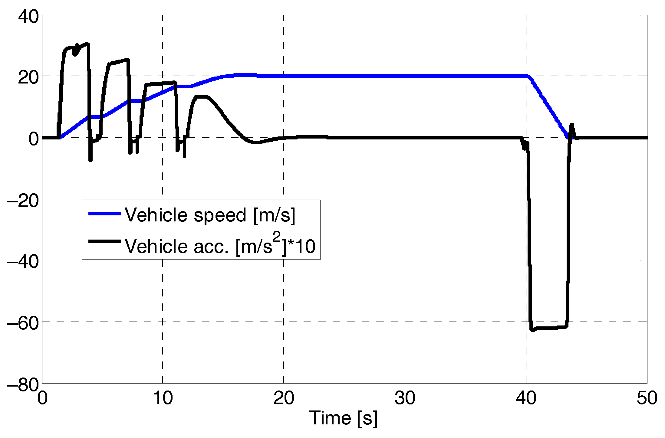
A straight line braking manoeuvre, reported in Figure 11, is simulated in IPG CarMaker environment. The simulated wheel force and torque profile are used as a reference to assess the prediction capability of the developed observer.
In Figure 12, the tire model and virtual sensor longitudinal forces are compared against the simulated reference value stemming from the IPG simulation software. It is noticeable that a good predictive capability is achieved by properly tuning the Kalman filter covariance matrices.
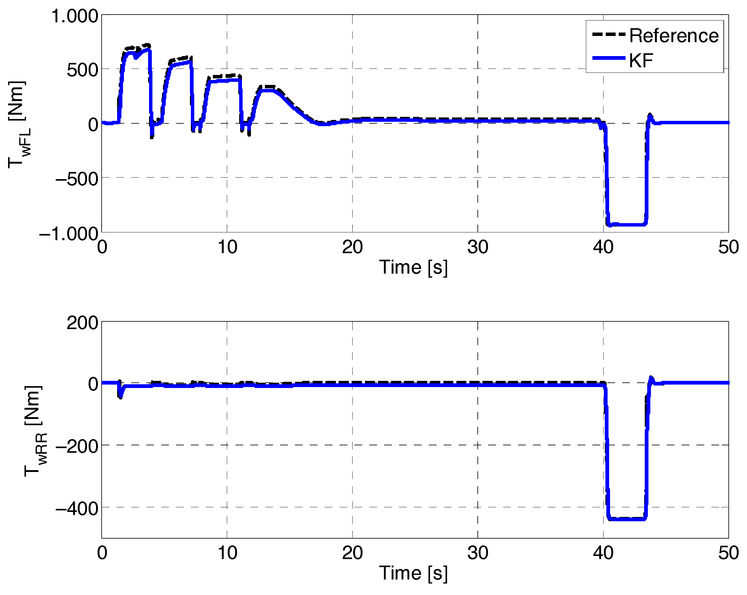
In Figure 13, the observed wheel torque is compared against the reference signal simulated in IPG. The Kalman filter is able to observe the wheel torque during both accelerating and decelerating phases with a RMSE (root-mean-square-error) underneath 30 Nm.
2.6. Conclusions
In the present work, a wheel torque observer has been proposed with the aim of estimating the BLCF. Thereafter, using Equation (18), it is simple to evaluate the actual BLCF once the wheel torque is observed, the clamping force is calculated from Equation (19) and the radial position of the clamping force application point is known.
The developed observer can also be used as support for several vehicle control systems. In particular, the state observation technique is expected to be a promising solution for brake control purposes: in comparison with the model-based approach and neural networks, it requires less computational burden and guarantees robustness since it does not require ad hoc identification of the specific plant. Considering all the mentioned drawbacks and the achieved results, it appears clear that the proposed state observer is a very powerful tool for online observation of the BLCF.
3. Conclusions
The goal of the present work is to identify a model capable of predicting the real BLCF in automotive disc brakes, by detailing the phenomena affecting the tribological contact, with the aim of monitoring the brake operation and its actuation for safety and environmental purposes. As surveyed, the ad hoc models for disc brakes are not capable of accurately predicting the BLCF for every operating condition. Indeed, it is noticeable that the brake operation is affected by several phenomena that make the friction hard to describe through conventional analytical models. In this regard, an auxiliary tool, the so-called cellular automata, is able to depict the correlation between the patch dynamics and wear particle stream and temperature has been presented. This model sets out to provide a guess of the frictional behaviour at the pad–disc contact and to find correlations between characteristics of friction and properties of the contacting materials and loading conditions. The integration of the cellular automata model with a friction law allows for offsetting the gap between the patch dynamics and the macroscopic phenomena. The great advantage of the cellular automata is that the complexity between the processes occurring on different time scales can be handled without complicating the employed model. This kind of simulation is very helpful to comprehend the particle flow on the small scale but, as remarked in the dedicated Section 2.3, conclusions about global friction behaviour are not possible.
Nonetheless, the brake wear [9] requires the inclusion of time dependence in the analytical form; the brake fading [5] demands the inclusion of a temperature-dependent term; the brake hysteresis [7] implies the use of a dynamic set of equations for the friction modelling. Owing to this complexity, the neural network has earned recent attention from the tribology community as an alternative approach to the achievement of a branched correlation between the friction and influencing factors such as pad composition, environmental conditions and operating conditions [77]. As evidenced, the approaches based on analytical correlations present several drawbacks that make them unsuitable for online applications:
- both the model-based approach and the neural networks require a high experimental burden for parameter characterization and the training/learning processes, respectively;
- both cause a high computational burden when augmented with differential equations modelling the brake disc temperature or the hysteresis behaviour;
- both become unreliable when the plant characteristics change due to brake wear itself or in the case of replacement with aftermarket brake linings and owing to a variation in the weather conditions.
Once it is clarified that an accurate modelling of all the friction phenomena is unknot likely to be achieved, from the literature it emerges that the design of an observer for the vehicle states has given rise to considerable interest among the control community, aimed at developing robust control strategies for brake enhancement during service operation. The state observation technique is expected to be a promising solution because:
- it uses measurements coming directly from the vehicle sensors by avoiding an analytical description of the brake phenomenology;
- it guarantees robustness since it does not need an ad hoc identification for the specific plant;
- it does not require the implementation of models that cause a high computational burden, such as brake temperature distribution models;
- finally, it can be used to predict the wheel torque as a supporting tool for the enhancement of the vehicle stability control systems.
Considering all the mentioned drawbacks and the achieved results, it appears clear that a state observer could be a very powerful tool for the online observation of BLCF. Hence, further research effort will be put into the design of an optimal observer for the improvement of driving safety, during emergency braking, and for the enhancement of brake actuation, during service braking, with simultaneous reduction of the wear and PM emissions.
Acknowledgments
This work has been carried out within the iTEAM (Interdisciplinary Training Network on Multi-Actuated Ground Vehicles), which receives funding from the European Community Horizon 2020 Framework Programme under grant agreement No. 675999. We acknowledge support for the Article Processing Charge by the German Research Foundation and the Open Access Publication Fund of the Technische Universität Ilmenau.
Author Contributions
The authorship is limited to those who have contributed substantially to the work realization. All the authors have participated to the design of experiments, analysis of data and results, and writing of the paper.
Conflicts of Interest
The authors declare no conflict of interest.
References
- UN ECE Regulations, No. 13-H, Uniform Provisions Concerning the Approval of Passenger Cars with Regard to Braking. 2010. Available online: http://eur-lex.europa.eu/legal-content/EN/ALL/?uri=CELEX:42010X0831(02) (accessed on 23 August 2016).
- Grigoratos, T.; Martini, G. Institute for Energy and Transport of the European Union, Non-Exhaust Traffic Related Emissions—Brake and Tire Wear PM. 2014. Available online: http://publications.jrc.ec.europa.eu/repository/bitstream/JRC89231/jrc89231-online%20final%20version%202.pdf (accessed on 23 August 2016).
- Augsburg, K.; Horn, R.; Sachse, H. Characterization of particulate emissions of vehicle wheel brakes. In Internationales Wissenschaftliches Kolloquium; Technische Universität Ilmenau: Ilmenau, Germany, 2011. [Google Scholar]
- Balotin, J.; Neis, P.; Ferreira, N. Analysis of the influence of temperature on the friction coefficient of friction materials. In ABCM Symposium Series in Mechatronics; Associação Brasileira de Engenharia e Ciências Mecânicas: Rio de Janeiro, Brasil, 2010. [Google Scholar]
- Talati, F.; Jalalifar, S. Analysis of heat conduction in a disk brake system. Heat Mass Transf. 2009, 45, 1047–1059. [Google Scholar] [CrossRef]
- Eriksson, M.; Bergman, F.; Jacobson, S. On the nature of tribological contact in automotive brakes. Wear 2002, 252, 26–36. [Google Scholar] [CrossRef]
- Shyrokau, B.; Wang, D.; Augsburg, K.; Ivanov, V. Vehicle Dynamics with Brake Hysteresis. Proc. Inst. Mech. Eng. Part D J. Automob. Eng. 2013, 227, 139–150. [Google Scholar] [CrossRef]
- Hess, D.; Soom, A. Friction at a lubricated line contact operating at oscillating sliding velocities. J. Tribol. 1990, 112, 147–152. [Google Scholar] [CrossRef]
- Thuresson, D. Thermomechanical analysis of friction brakes. SAE Tech. Pap. 2000, 149–159. [Google Scholar] [CrossRef]
- Blau, P.J. Embedding wear models into friction models. Tribol. Lett. 2009, 34, 75–79. [Google Scholar] [CrossRef]
- Chan, D.; Stachowiak, W. Review of automotive brake friction materials. Proc. Inst. Mech. Eng. Part D J. Automob. Eng. 2004, 218, 953–963. [Google Scholar] [CrossRef]
- Nagesh, S.; Siddaraju, C.; Prakash, S.; Ramesh, M. Characterization of brake pads by variation in composition of friction materials. Proc. Mater. Sci. 2014, 5, 295–302. [Google Scholar] [CrossRef]
- Soom, A.; Kim, C. Interaction between dynamic normal and frictional forces during unlubricated sliding. J. Lubr. Technol. 1983, 105, 221–229. [Google Scholar] [CrossRef]
- Verma, P.C.; Ciudin, R.; Bonfanti, A.; Aswath, P.; Straffelini, G.; Gialanella, S. Role of the friction layer in the high-temperature pin-on-disc study of a brake material. Wear 2016, 346, 56–65. [Google Scholar] [CrossRef]
- Straffelini, G.; Verlinski, S.; Verma, P.C.; Valota, G.; Gialanella, S. Wear and Contact Temperature Evolution in Pin-on-Disc Tribotesting of Low-Metallic Friction Material Sliding Against Pearlitic Cast Iron. Tribol. Lett. 2016, 62, 1–11. [Google Scholar] [CrossRef]
- Dahl, P. A Solid Friction Model; Technical Report TOR-0158(3107-18)-1; The Aerospace Corporation: El Segundo, CA, USA, 1968. [Google Scholar]
- Ostermeyer, G. On the dynamics of the friction coefficient. Wear 2003, 254, 852–858. [Google Scholar] [CrossRef]
- Eriksson, M.; Lundqvist, A.; Jacobson, S. A study of the influence of humidity on the friction and squeal generation of automotive brake pads. Proc. Inst. Mech. Eng. Part D J. Automob. Eng 2011, 215, 329–342. [Google Scholar] [CrossRef]
- Eriksson, M.; Bergman, F.; Jacobson, S. Surface characterisation of brake pads after running under silent and squealing conditions. Wear 1999, 232, 163–167. [Google Scholar] [CrossRef]
- Kim, M. Development of the braking performance evaluation technology for high speed brake dynamometer. Int. J. Syst. Appl. Eng. Dev. 2012, 6, 122–129. [Google Scholar]
- Rus, D.; Capitanu, L.; Badita, L.L. A qualitative correlation between friction coefficient and steel surface wear in linear dry sliding contact to polymers with SGF. Friction 2014, 2, 47–57. [Google Scholar] [CrossRef]
- Berger, E.J. Friction modeling for dynamic system simulation. Appl. Mech. Rev. 2002, 55, 535–577. [Google Scholar] [CrossRef]
- Awrejcewicz, J.; Olejnik, P. Analysis of dynamic systems with various friction laws. Appl. Mech. Rev. 2005, 58, 389–411. [Google Scholar] [CrossRef]
- Akay, A. Acoustics of friction. J. Acoust. Soc. Am. 2002, 111, 1525–1548. [Google Scholar] [CrossRef] [PubMed]
- Panteley, E.; Ortega, R.; Gäfvert, M. An adaptive friction compensator for global tracking in robot manipulators. Syst. Control Lett. 1998, 33, 307–313. [Google Scholar] [CrossRef]
- Armstrong, B.; Dupont, P.; de Wit, C.C. A survey of models, analysis tools and compensation methods for the control of machines with friction. Automatica 1994, 30, 1083–1138. [Google Scholar] [CrossRef]
- Hayward, V.; Armstrong, B.S.; Altpeter, F.; Dupont, P. Discrete time elasto-plastic friction estimation. IEEE Trans. Control Syst. Technol. 2009, 17, 688–696. [Google Scholar] [CrossRef]
- Stribeck, R. The key qualities of sliding and roller bearings. Z. Ver. Seutscher Ing. 1902, 46, 1432–1437. [Google Scholar]
- Hunt, J.; Torbe, I.; Spencer, G. The phase plane analysis of sliding motion. Wear 1965, 8, 455–465. [Google Scholar] [CrossRef]
- Anderson, J.; Ferri, A. Behavior of a single degree of freedom system with a generalized friction law. J. Sound Vib. 1990, 140, 287–304. [Google Scholar] [CrossRef]
- Matozo, L.; Soares, M.; Al-Qureshi, H. The effect of environmental humidity and temperature on friction level and squeal noise propensity for disc brake friction materials. SAE Int. 2008. [Google Scholar] [CrossRef]
- Okamura, T. Effect of directional surface finish of brake discs on friction behavior during running-in. SAE Int. J. Passeng. Cars Mech. Syst. 2011, 4, 1445–1452. [Google Scholar] [CrossRef]
- Shyrokau, B.; Savitski, D.; Wang, D.; Ivanov, V.; Augsburg, K. Analysis of coordination and novel blending strategy between friction brake system and electric motors. In EuroBrake; FISITA: Dresden, Germany, 2013. [Google Scholar]
- Crolla, D.; Lang, A. Brake noise and vibrations—The state of the art. Tribol. Ser. 1991, 18, 165–174. [Google Scholar]
- Drakunov, S. ABS Control using optimum search via sliding modes. IEEE Trans. Control Syst. Technol. 1995, 3, 79–85. [Google Scholar] [CrossRef]
- Shin, K.; Brennan, M.; Oh, J.; Harris, C. Analysis of disc brake noise using a two-degree-of-freedon model. J. Sound Vib. 2002, 254, 837–848. [Google Scholar] [CrossRef]
- Kragelsky, I.V.; Dobychin, M.N.; Kombalov, V.S. Friction and Wear: Calculation Methods; Elsevier: Amsterdam, The Netherlands, 2013. [Google Scholar]
- Al-Bender, F. Fundamentals of friction modeling. In Proceedings of the ASPE Spring Topical Meeting on Control of Precision Systems, Cambridge, MA, USA, 11–13 April 2010. [Google Scholar]
- Kang, J.; Chois, S. Brake dynamometer model predicting brake torque variation due to disc thickness variation. Proc. Insit. Mech. Eng. Part D J. Automob. Eng. 2007, 221, 49–55. [Google Scholar] [CrossRef]
- Behrendt, J.; Weiss, C.; Hoffmann, N. A numerical study on stick-slip motion of a brake pad in steady sliding. J. Sound Vib. 2011, 330, 636–651. [Google Scholar] [CrossRef]
- Grkic, A.; Muzdeka, S.; Arsenic, Z.; Duboka, C. Model for estimation of the friction coefficient in automotive brakes under extremely high temperatures. Int. J. Eng. Tech. Res. 2014, 2, 290–294. [Google Scholar]
- Lee, N.; Kang, C. The effect of a variabble disc pad friction coefficient for the mechanical brake system of a railway vehicle. PLoS ONE 2015, 10, e0135459. [Google Scholar]
- Martinez, C.; Velenis, E.; Tavernini, D.; Gao, B. Modelling and estimation of friction brake torque for a brake by wire system. In Proceedings of the 2014 IEEE International Electric Vehicle Conference (IEVC), Florence, Italy, 17–19 December 2014. [Google Scholar]
- Shangshuai, J.; Li, O. Friction induced vibration and noise on a brake system. In Proceedings of the 2013 IEEE International Conference Information and Automation (ICIA), Yinchuan, China, 26–28 August 2013. [Google Scholar]
- Wan, Z.; Liu, X.; Wang, H.; Shan, Y.; He, T. Friction Coefficient Model of Friction Pair Composed of Automotive Brake Materials. ASME 2014. [Google Scholar] [CrossRef]
- Loh, W.Y.; Basch, R.H.; Li, D.; Sanders, P. Dynamic modeling of brake friction coefficients. SAE Int. 2000. [Google Scholar] [CrossRef]
- Oberst, S.; Lai, J.C.S. Numerical study of friction induced pad mode instability in disc brake squeal. In Proceedings of the 20th International Congress on Acoustics, Sydney, Australia, 23–27 August 2010; pp. 23–27. [Google Scholar]
- Mohammed, A.; Rahim, I. Disc plate squeal investigation using finite element software: Study and compare. Int. J. Sci. Technol. Res. 2013, 2, 2277–8616. [Google Scholar]
- Söderberg, A.; Sören, A. Simulation of wear and contact pressure distribution at the pad to rotor interface in a disc brake using general pupose finite element analysis software. Wear 2009, 267, 2243–2251. [Google Scholar] [CrossRef]
- Wang, K.; Tang, J. Analysis of thermanl mechanical coupling of automotive disc brake based on numerical simulation method. Open Mech. Eng. J. 2015, 9, 28–33. [Google Scholar] [CrossRef]
- Chichinadze, A.; Braun, E. Ginsburg, Calculation, Test and Selection of Frictional Couples; Nauka: Moscow, Russia, 1979. (In Russian) [Google Scholar]
- Cheney, W.; Kincaid, D. Numerical Mathematics and Computing; Thomson Brooks, Cole: Monterey, CA, USA, 2008. [Google Scholar]
- Von Neumann, J.; Burks, A. Theory of self-reproducing automata. IEEE Trans. Neural Netw. 1966, 5, 3–14. [Google Scholar]
- Ostermeyer, G.; Müller, M. New insights into the tribology of brake systems. Proc. Inst. Mech. Eng. Part D J. Automob. Eng. 2008, 7, 1167–1200. [Google Scholar] [CrossRef]
- Müller, M.; Ostermeyer, G. A Cellular Automaton Model for Tribological Problems. In Proceedings of the International Conference on Cellular Automata, Perpignan, France, 20–23 September 2008; pp. 92–99. [Google Scholar]
- Müller, M.; Ostermeyer, G. A Cellular Automaton model to describe the three-dimensional friction and wear mechanism of brake systems. Wear 2007, 263, 1175–1188. [Google Scholar] [CrossRef]
- Wahlström, J.; Söderberg, A.; Olofsson, U. A cellular automaton approach to numerically simulate the contact situation in disc brakes. Tribol. Lett. 2011, 42, 253–262. [Google Scholar] [CrossRef]
- Österle, W.; Kloß, H.; Urban, I.; Dmitriev, A. Towards a better understanding of brake friction materials. Wear 2007, 263, 1189–1201. [Google Scholar] [CrossRef]
- Dmitriev, A.; Österle, W. Modeling of brake pad-disc interface with emphasis to dynamics and deformation of structures. Tribol. Int. 2010, 43, 719–727. [Google Scholar] [CrossRef]
- Ćirović, V.; Aleksendrić, D. Development of neural network model of disc brake operation. FME Trans. 2010, 38, 29–38. [Google Scholar]
- Aleksendric, D.; Duboka, C. Prediction of automotive friction material characteristics using artificial neural networks-cold performance. Wear 2006, 261, 269–282. [Google Scholar] [CrossRef]
- Senatore, A.; D’Agostino, V.; di Guida, R.; Petrone, V. Experimental investigation and neural network prediction of brake and clutch material frictional behaviour considering the sliding acceleration influence. Tribol. Int. 2011, 44, 1199–1207. [Google Scholar] [CrossRef]
- Yin, Y.; Bao, J.; Yang, L. Tribological properties prediction of brake lining for automobiles based on BP neural network. In Proceedings of the Control and Decision Conference, Xuzhou, China, 26–28 May 2010. [Google Scholar]
- Mutlu, I. Artificial neural network modelling of non-asbestos brake lining performance boric acid in brake pad. Inf. Technol. J. 2009, 8, 389–402. [Google Scholar] [CrossRef]
- Aleksendrić, D.; Barton, D.C. Neural network prediction of disc brake performance. Tribol. Int. 2009, 42, 1074–1080. [Google Scholar] [CrossRef]
- Ćirović, V.; Aleksendrić, D. Dynamic modeling of disc brake contact phenomena. FME Trans. 2011, 39, 177–183. [Google Scholar]
- Savitski, D.; Ivanov, V.; Heidrich, L.; Augsburg, K.; Pütz, T. Experimental investigation of braking dynamics of electric vehicles. In EuroBrake; FISITA: Dresden, Germany, 2013. [Google Scholar]
- Ray, L. Nonlinear tire force estimation and road friction identification: Simulation and experiments. Automatica 1997, 33, 1819–1833. [Google Scholar] [CrossRef]
- Müller, S.; Uchanski, M.; Heidrick, K. Estimation of the maximum tire-road friction coefficient. J. Dyn. Syst. Meas. Control 2003, 154, 607–617. [Google Scholar] [CrossRef]
- Rajamani, R.; Phanomchoeng, G.; Piyabongkarn, D.; Lew, J.Y. Algorithms for real-time estimation of individual wheel tire-road friction coefficients. IEEE/ASME Trans. Mechatron. 2012, 17, 1183–1195. [Google Scholar] [CrossRef]
- Doumiati, M.; Victorino, A.; Charara, A.; Lechner, D. Estimation of vehicle lateral tire-road forces: A comparison between extended and unscented kalman filtering. In Proceedings of the 2009 European Control Conference (ECC), Budapest, Hungary, 23–26 August 2009; pp. 4804–4809. [Google Scholar]
- Hamann, H.; Heidrick, J.K.; Rhode, S.; Gauterin, F. Tire force estimation for a passenger vehicle with the unscented kalman filter. In Proceedings of the 2014 IEEE Intelligent Vehicles Symposium Proceedings, Dearborn, MI, USA, 8–11 June 2014; pp. 814–819. [Google Scholar]
- Ricciardi, V.; Augsburg, K.; Ivanov, V. A novel approach for the estimation of the brake friction coefficient for environmental and safety control applications. In EuroBrake; FISITA: Dresden, Germany, 2017. [Google Scholar]
- Hostetter, G.H.; Meditch, J.S. On the generalization of observers to systems with unmeasurable, unknown inputs. Automatica 1973, 9, 721–724. [Google Scholar] [CrossRef]
- Kiencke, U.; Nielsen, L. Automotive Control Systems: For Engine, Driveline, and Vehicle; Springer: Berlin, Germany, 2005. [Google Scholar]
- Doumiati, M.; Victorino, A.; Charara, A.; Baffet, G.; Lechner, D. An estimation process for vehicle wheel-ground contact normal forces. IFAC Proc. Vol. 2008, 41, 7110–7115. [Google Scholar] [CrossRef]
- Xiao, X.; Yin, Y.; Bao, J.; Lu, L.; Feng, X. Review on the friction and wear of brake materials. Adv. Mech. Eng. 2016, 8. [Google Scholar] [CrossRef]
Figure 1.
Pie chart arising of the state of art of techniques for the estimation of the BLCF.

Figure 2.
Energetic balance involving friction phenomena, as proposed in [17]. Reprinted with permission from [17]. Copyright Elsevier, 2003.

Figure 3.
Brake dynamometer with climatic chamber, employed for experimental tests at the Technische Universität Ilmenau. 1—Drive Motor, 2—Flywheels, 3—Inertial hub, 4—Torque sensor, 5—Brake disc, 6—Brake calliper, 7—Brake pressure sensor, 8—Flow meter, 9—Master cylinder, 10—Compressed air hydraulic actuator, 11—Pressure accumulator.

Figure 4.
Experimental measurements on the brake test rig performed at TU Ilmenau. Datasets (a) and (b) have been used for the identification and validation procedures, respectively. Top row: the oscillating braking pressure, as an input of the system. Middle row: brake speed profile. Bottom row: brake temperature profile.

Figure 5.
(a) Results of the identification process (first dataset); (b) results of the validation process (second dataset). Comparison between the experimental and the model-predicted braking torque.
Figure 5.
(a) Results of the identification process (first dataset); (b) results of the validation process (second dataset). Comparison between the experimental and the model-predicted braking torque.

Figure 6.
The measurements of the first dataset show a memory effect (hysteresis) of BLCF against the braking pressure and a clear dependence of the resulting braking torque on rising temperature. The model is capable of capturing the temperature dependence but not the frictional lag against the pressure.

Figure 7.
Cellular automata discretization and portrayal of the patch structures in black [54].
Figure 7.
Cellular automata discretization and portrayal of the patch structures in black [54].

Figure 8.
Characteristic times for the multi-scale problem in analysis [56].
Figure 8.
Characteristic times for the multi-scale problem in analysis [56].

Figure 9.
Artificial neural network for BLCF estimation.

Figure 10.
Structure of the proposed KF: the update part is based on the measurements coming from the hub sensors and the accelerometers; the prediction part relies on the wheels’ dynamics equations and on the tire model, which, in turn, requires the tire slip ratios and the vertical load.
Figure 10.
Structure of the proposed KF: the update part is based on the measurements coming from the hub sensors and the accelerometers; the prediction part relies on the wheels’ dynamics equations and on the tire model, which, in turn, requires the tire slip ratios and the vertical load.

Figure 11.
Straight line braking manoeuvre. The blue profile represents the actual vehicle speed and the black curve is the vehicle longitudinal acceleration.
Figure 11.
Straight line braking manoeuvre. The blue profile represents the actual vehicle speed and the black curve is the vehicle longitudinal acceleration.

Figure 12.
The chassis longitudinal force predicted from the tire model and virtually measured compared to the simulated profile.
Figure 12.
The chassis longitudinal force predicted from the tire model and virtually measured compared to the simulated profile.

Figure 13.
Comparison between the simulated wheel torque in IPG CarMaker (Reference) and the observed value (KF) for the front left wheel (above) and the rear right wheel (below).
Figure 13.
Comparison between the simulated wheel torque in IPG CarMaker (Reference) and the observed value (KF) for the front left wheel (above) and the rear right wheel (below).


Table 1.
Vehicle parameters used for the simulation.
| Powertrain Type | FWD | Tyre Size | 195/65 R15 |
|---|---|---|---|
| Parameter | Value | Parameter | Value |
| mv | 1463 kg | i2 | 1.9 |
| ms | 1301 kg | i3 | 1.35 |
| Iz | 1800 kg m2 | i4 | 1.05 |
| Iω | 1 kg m2 | i5 | 0.8 |
| Rω | 0.31 m | idiff | 4.1 |
| i1 | 3.4 | hcg | 0.58 m |
© 2017 by the authors. Licensee MDPI, Basel, Switzerland. This article is an open access article distributed under the terms and conditions of the Creative Commons Attribution (CC BY) license (http://creativecommons.org/licenses/by/4.0/).
Share and Cite
MDPI and ACS Style
Ricciardi, V.; Augsburg, K.; Gramstat, S.; Schreiber, V.; Ivanov, V. Survey on Modelling and Techniques for Friction Estimation in Automotive Brakes. Appl. Sci. 2017, 7, 873. https://doi.org/10.3390/app7090873
AMA Style
Ricciardi V, Augsburg K, Gramstat S, Schreiber V, Ivanov V. Survey on Modelling and Techniques for Friction Estimation in Automotive Brakes. Applied Sciences. 2017; 7(9):873. https://doi.org/10.3390/app7090873
Chicago/Turabian StyleRicciardi, Vincenzo, Klaus Augsburg, Sebastian Gramstat, Viktor Schreiber, and Valentin Ivanov. 2017. "Survey on Modelling and Techniques for Friction Estimation in Automotive Brakes" Applied Sciences 7, no. 9: 873. https://doi.org/10.3390/app7090873
Note that from the first issue of 2016, this journal uses article numbers instead of page numbers. See further details here.