Hierarchical Colored Petri Nets for Modeling and Analysis of Transit Signal Priority Control Systems


Abstract
:1. Introduction
2. Transit Priority Signalized Intersection
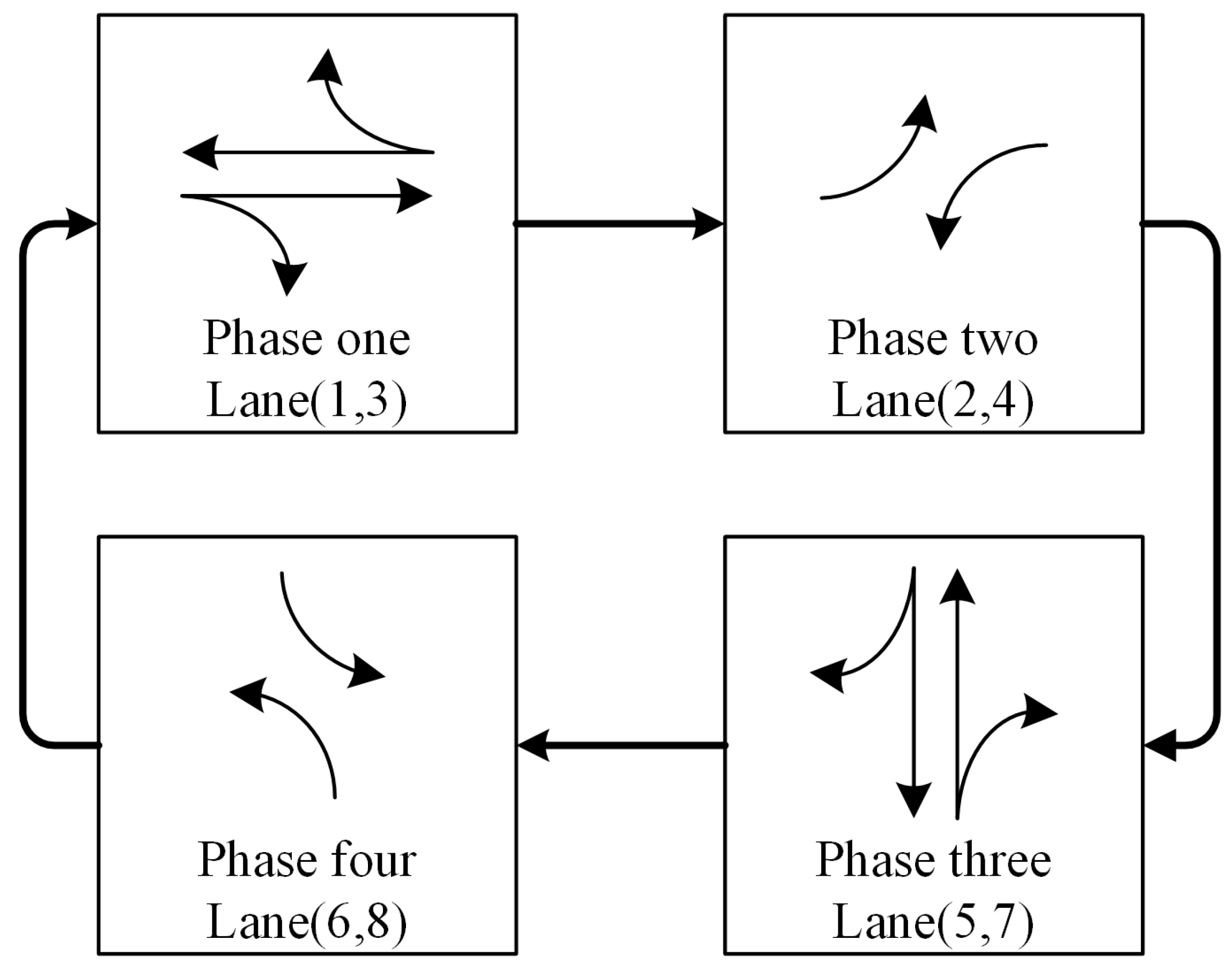
2.1. Signalized Intersection
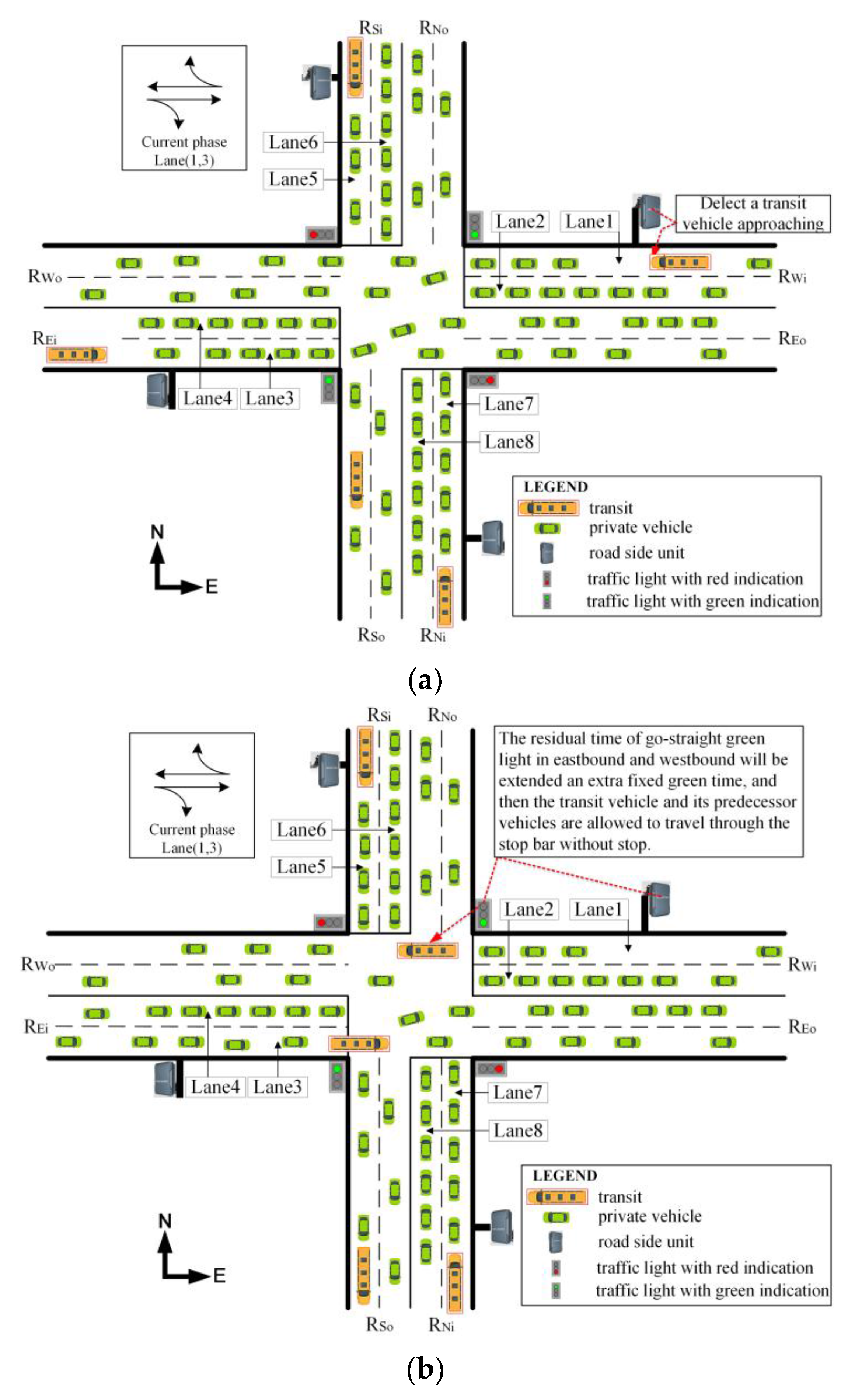
2.2. Transit Detection
2.3. Transit Signal Priority Control
3. Petri Net Representation
3.1. HCPN Concepts
- 1.
- is a finite set of places;
- 2.
- is a finite set of transitions and ;
- 3.
- is a finite set of directed arcs, ;
- 4.
- is a finite set of non-empty color sets;
- 5.
- is a set of typed variables, such that ;
- 6.
- is a color set function that assigns a color set to each place;
- 7.
- is a guard function that assigns a guard to each transition such that ;
- 8.
- is an arc expression function that assigns an arc expression to each arc a such that , here, means multiset;
- 9.
- is an initialization function that assigns an initialization expression to each place p such that .
- 1.
- is a non-hierarchical colored Petri net;
- 2.
- is a set of substitution transitions;
- 3.
- is a set of port places;
- 4.
- is a port type function that assigns a port type to each port place.
- 1.
- is a finite set of modules. Each module is a Colored Petri net module , it is required that for all such that ;
- 2.
- is a submodule function that assigns a sub module to each substitution transition. It is required that the module hierarchy is acyclic;
- 3.
- is a port-socket relation function that assigns a port-socket relation to each substitution transition , it is required that , and for all and all ;
- 4.
- is a set of non-empty fusion sets such that and for all and all .
3.2. Assumptions and Rules
- In the urban traffic network, when one vehicle is approaching to an intersection, usually, the driver prefers to decelerate the vehicle and ensures that the vehicle safely passes through the intersection or waits in a queue. Hence, we set the nominal travel speed at km/h, and the RSU sensor for transit detection is deployed at a distance of from the stop bar;
- In each phase, the traffic lights turn on in the following order: green lights for seconds, yellow lights for seconds, and red lights for seconds. In order to ensure safety, when a cycle is completed, all-in-red lights turn on for seconds. Therefore, a complete signal cycle is seconds;
- The event that the RSU sensor detects an approaching transit vehicle is stochastic and uncertain, but the traffic signal controller’s response to the event is deterministic. Therefore, to cope with the complexity of the TSP control model, it is crucial to reduce some redundant states while a full state space is constructed and analyzed.
- If the traffic signal controller receives more than two green extension requests in each phase, these requests are handled in accordance to the principle that only the first one is served and the others are neglected;
- The same principle can be used to the two or more red truncation requests;
- If the controller receives two different requests at the same time, the response to the green extension request is superior to the response to the red truncation request.
3.3. Green Extension Strategy
- The residual green time when a transit vehicle is detected is expressed as . The additional green time is set to ;
- The distance between the RSU sensor installed on the road side and the stop bar is expressed as . The nominal speed of the transit vehicle is expressed as , when it is detected by the RSU sensor. The estimated time to travel to the stop bar is expressed as ;
- When a TSP request is received by the controller in the current phase, it checks whether the detected transit vehicle has enough green time to travel to the stop bar or not, there are four cases should be considered:
- Case 1.
- If the condition holds, it means that the transit vehicle will travel through the intersection without delay.
- Case 2.
- If the condition holds, it means that the yellow light will turn on and the transit vehicle has to wait for the green light in next cycle before the stop bar.
- Case 3.
- For Case 2, if the formula is also satisfied, then an additional green time () can be appended to the residual green time such that the new remaining green time is long enough to serve the transit vehicle during this phase.
- Case 4.
- If the condition and holds, it means that the original residual green is between one to and is not long enough to serve this vehicle during this phase either. In this situation, even if an additional green time is appended, the transit vehicle has to wait until the next cycle.
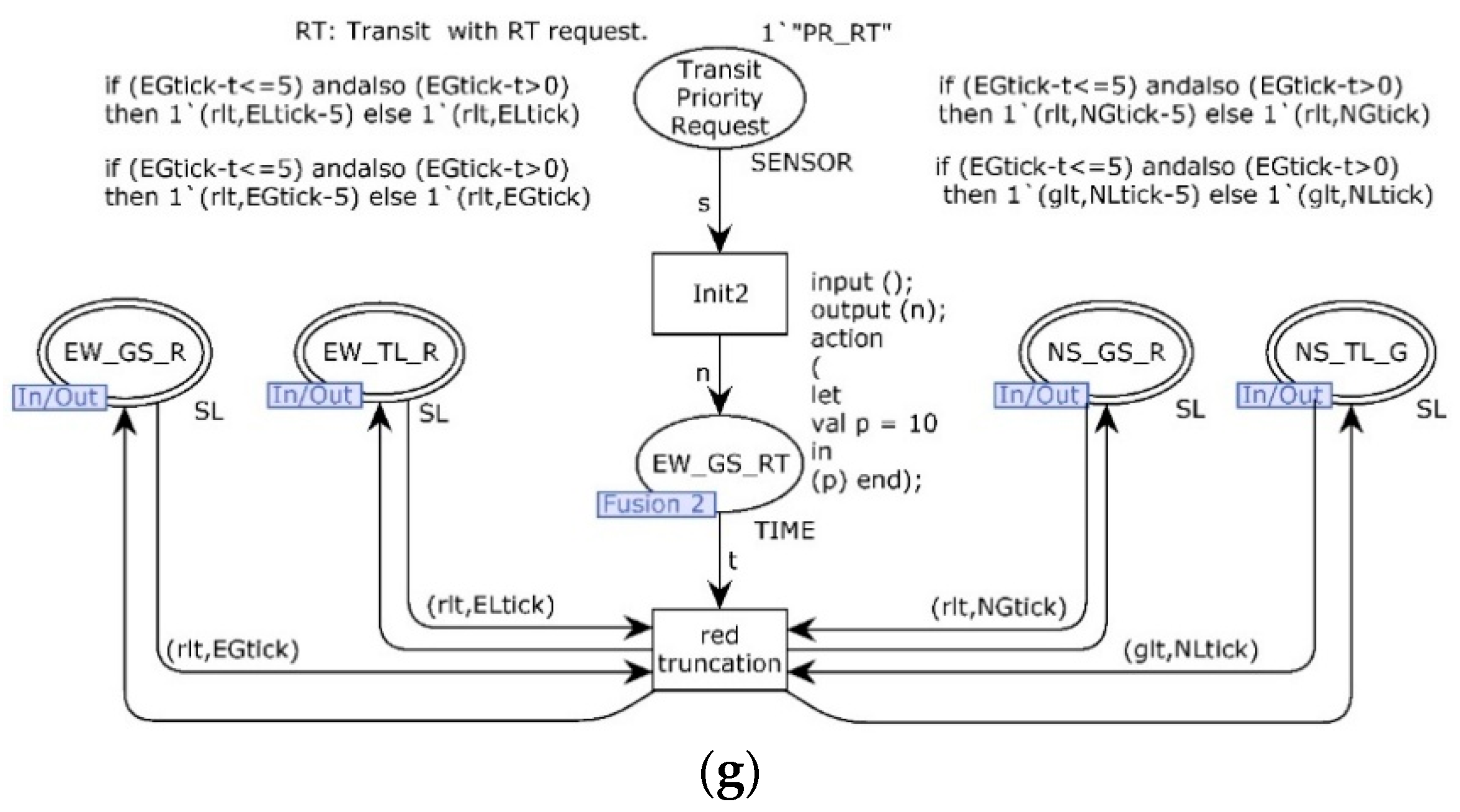
3.4. Red Truncation Strategy
- The residual red time when a transit vehicle is detected is expressed as . The threshold of red time to be truncated is set to ;
- The three parameters , , have the same meaning as in Section 3.3;
- When a TSP request is received by the controller in the current phase, it checks if the detected transit vehicle needs to stop at least once. The more detailed information is summarized into four cases as follows.
- Case 1.
- If the condition is satisfied, it means that the traffic signal will turn green before the transit vehicle travels to the stop bar.
- Case 2.
- If the condition holds, it means that the detected transit vehicle need to stop at least once.
- Case 3.
- For Case 2, if the formula is also satified, then a fixed period of red time () can be truncated from the current phase. Then, the new remaining red time () is guaranted such that this transit vehicle can travel through the stop bar without any stop.
- Case 4.
- If the condition holds, it means that the residual red time is quite long, beyond the adjustment range. Hence, the transit vehicle has to wait before the stop bar until the red light turns green.
3.5. General Modeling Methodology
- Inputs:
- An intersection with TSP requirements, RSUs.
- Output:
- A HCPN-based TSP control model.
- Steps:
- (1) Identify the main states of the signal control system and its transitions.(2) Define the colorset, variable, and functions used in the potential CPN model.(3) Design the four-phase (or two-phase, six-phase) traffic signal control CPN model.(4) Using the hierarchical method, transform the CPN model into the HCPN model.(5) Construct two HCPN submodules based on two proposed TSP strategies, and integrated into the HCPN model.(6) According to the application requirements, set the following parameters: , , , , , , , .(7) Simulate and refine the HCPN-based TSP control model.(8) Analyze the HCPN-based TSP control model.
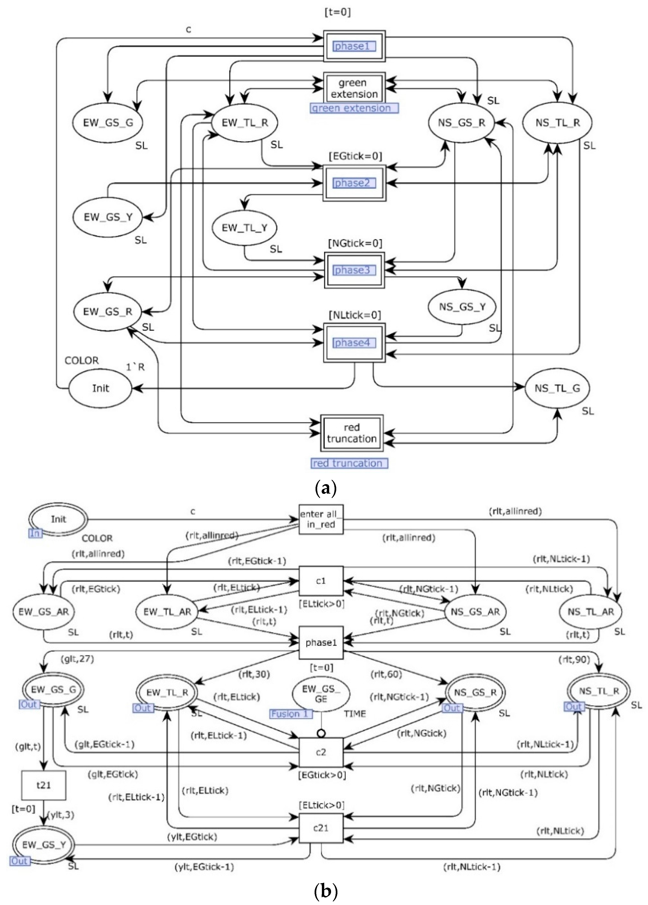
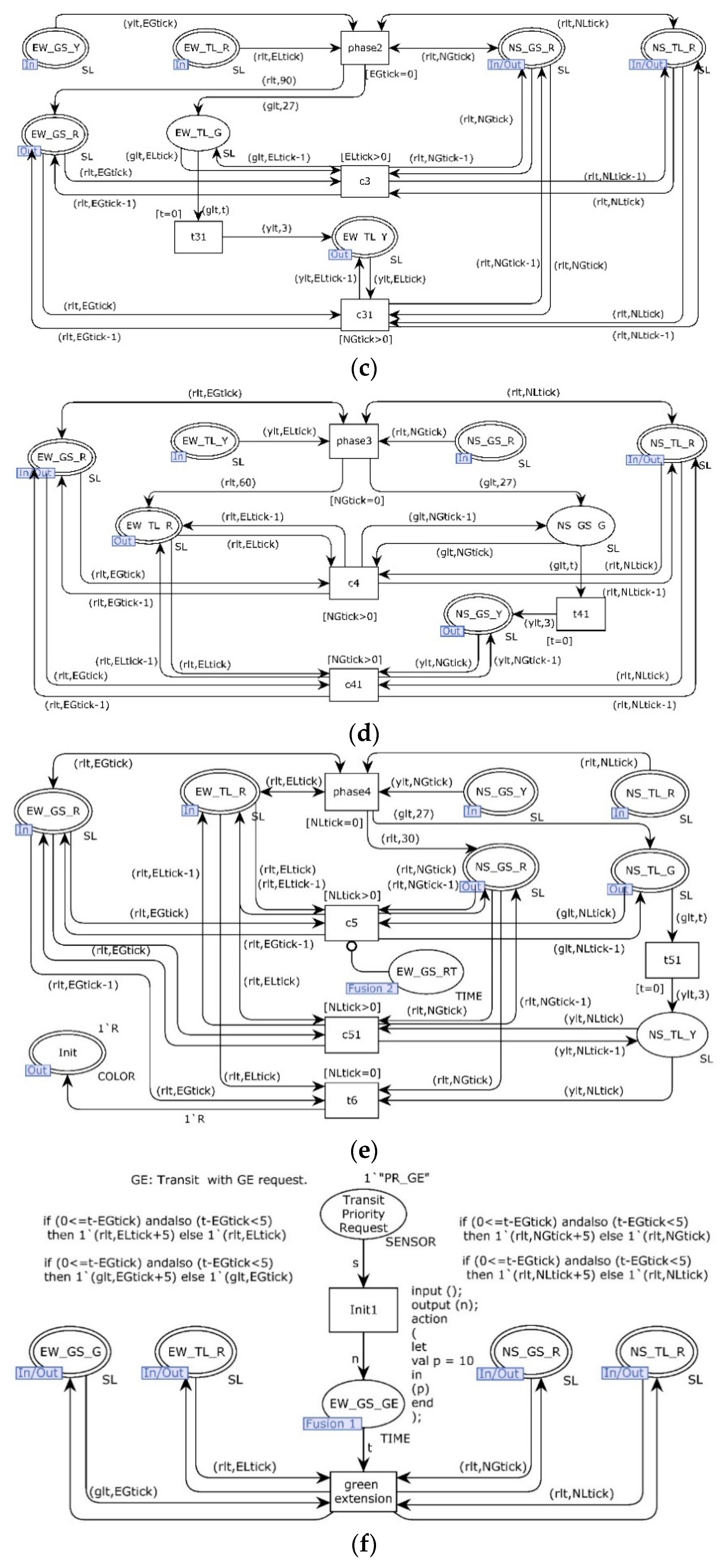
3.6. Transit Signal Priority Control Model
- if (0<=t-EGtick) andalso (t-EGtick < 5) then 1’(glt,EGtick + 5) else 1’(glt,EGtick)
- if (0<=t-EGtick) andalso (t-EGtick < 5) then 1’(rlt,ELtick + 5) else 1’(rlt,ELtick)
- if (0<=t-EGtick) andalso (t-EGtick < 5) then 1’(rlt,NGtick + 5) else 1’(rlt,NGtick)
- if (0<=t-EGtick) andalso (t-EGtick < 5) then 1’(rlt,NLtick + 5) else 1’(rlt,NLtick)
4. Simulation and Analysis of HCPN Based TSP Model
4.1. Simulation of HCPN Based TSP Model
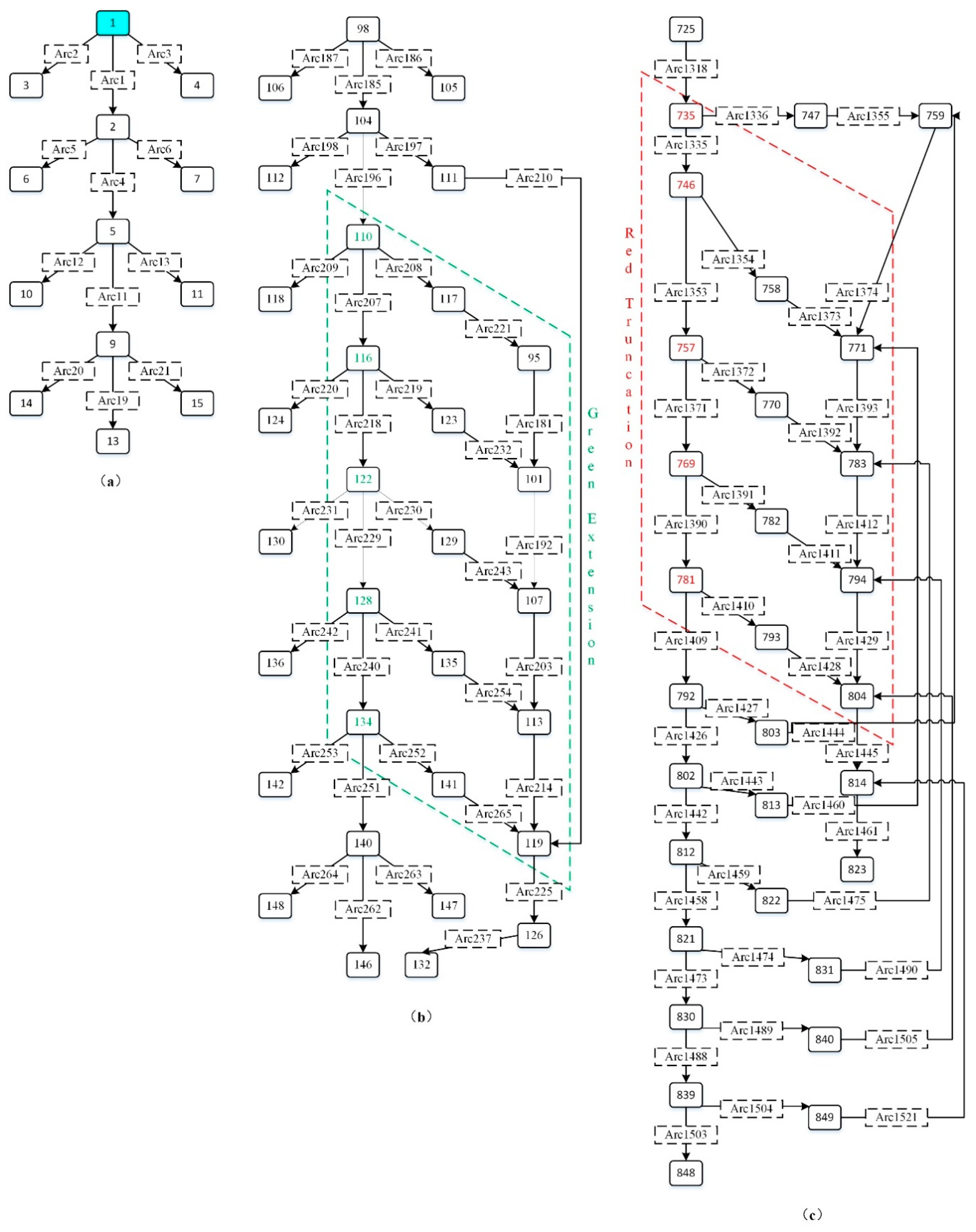
4.2. State Space Analysis
- Arc1:1→2 (phase1’enter_all_in_red:{c=R})
- Arc2:1→3 (green_extension’Init1:{s=”Bus Request GE”, n=10})
- Arc3:1→4 (red_truncation’Init2:{s=”Bus Request RT”, n=10})
- Arc4:2→5 (phase1’c1:{EGtick=2, ELtick=2, NGtick=2, NLtick=2})
- Arc11:5→9 (phase1’c1:{EGtick=1, ELtick=1, NGtick=1, NLtick=1})
4.3. Case Study
5. Conclusions
Acknowledgments
Author Contributions
Conflicts of Interest
Appendix A
Appendix B
Appendix B.1. Arcs Used in Figure 4a
- Arc1:1→2 phase1’enter_all_in_red:{c=R}
- Arc2:1→3 green_extension’Init1:{s=”PR_GE”, n=10}
- Arc3:1→4 red_truncation’Init2:{s=”PR_RT”, n=10}
- Arc4:2→5 phase1’c1:{EGtick=2, ELtick=2, NGtick=2, NLtick=2}
- Arc5:2→6 green_extension’Init1:{s=”PR_GE”, n=10}
- Arc6:2→7 red_truncation’Init2:{s=”PR_RT”, n=10}
- Arc11:5→9 phase1’c1:{EGtick=1, ELtick=1, NGtick=1, NLtick=1}
- Arc12:5→10 green_extension’Init1:{s=”PR_GE”, n=10}
- Arc13:5→11 red_truncation’Init2:{s=”PR_RT”, n=10}
- Arc19:9→13 phase1’phase1:{t=0}
- Arc20:9→14 green_extension’Init1:{s=”PR_GE”, n=10}
- Arc21:9→15 red_truncation’Init2:{s=”PR_RT”, n=10}
Appendix B.2. Arcs Used in Figure 4b
- Arc181:95→101 phase1’c2:{EGtick=15, ELtick=18, NGtick=48, NLtick=78}
- Arc185:98→104 phase1’c1:{EGtick=12, ELtick=15, NGtick=45, NLtick=75}
- Arc186:98→105 green_extension’Init1:{s=”PR_GE”, n=10}
- Arc187:98→106 red_truncation’Init2:{s=”PR_RT”, n=10}
- Arc192:101→107 phase1’c2:{EGtick=14, ELtick=17, NGtick=47, NLtick=77}
- Arc196:104→110 phase1’c2:{EGtick=11, ELtick=14, NGtick=44, NLtick=74}
- Arc197:104→111 green_extension’Init1:{s=”PR_GE”, n=10}
- Arc198:104→112 red_truncation’Init2:{s=”PR_RT”, n=10}
- Arc203:107→113 phase1’c2:{EGtick=13, ELtick=16, NGtick=46, NLtick=76}
- Arc207:110→116 phase1’c2:{EGtick=10, ELtick=13, NGtick=43, NLtick=73}
- Arc208:110→117 green_extension’Init1:{s=”PR_GE”, n=10}
- Arc209: 110→118 red_truncation’Init2:{s=”PR_RT”, n=10}
- Arc210:111→119 green_extension’green_extension:{EGtick=11, NGtick=44, ELtick=14, NLtick=74, t=10}
- Arc214:113→119 phase1’c2:{EGtick=12, ELtick=15, NGtick=45, NLtick=75}
- Arc218:116→122 phase1’c2:{EGtick=9, ELtick=12, NGtick=42, NLtick=72}
- Arc219:116→123 green_extension’Init1:{s=”PR_GE”, n=10}
- Arc220:116→124 red_truncation’Init2:{s=”PR_RT”, n=10}
- Arc221:117→95 green_extension’green_extension:{EGtick=10, ELtick=13, NGtick=43, NLtick=73, t=10}
- Arc225:119→126 phase1’c2:{EGtick=11, ELtick=14, NGtick=44, NLtick=74}
- Arc229:122→128 phase1’c2:{EGtick=8, ELtick=11, NGtick=41, NLtick=71}
- Arc230:122→129 green_extension’Init1:{s=”PR_GE”, n=10}
- Arc231: 122→130 red_truncation’Init2:{s=”PR_RT”, n=10}
- Arc232:123→101green_extension’green_extension:{EGtick=9, ELtick=12, NGtick=42, NLtick=72, t=10}
- Arc237:126→132 phase1’c2:{EGtick=10, ELtick=13, NGtick=43, NLtick=73}
- Arc240:128→134 phase1’c2:{EGtick=7, ELtick=10, NGtick=40, NLtick=70}
- Arc241:128→135 green_extension’Init1:{s=”PR_GE”, n=10}
- Arc242: 128→136 red_truncation’Init2:{s=”PR_RT”, n=10}
- Arc243:129→107 green_extension’green_extension:{EGtick=8, ELtick=11, NGtick=41, NLtick=71, t=10}
- Arc251:134→140 phase1’c2:{EGtick=6, ELtick=9, NGtick=39, NLtick=69}
- Arc252:134→141 green_extension’Init1:{s=”PR_GE”, n=10}
- Arc253:134→142 red_truncation’Init2:{s=”PR_RT”, n=10}
- Arc254:135→113 green_extension’green_extension:{EGtick=7, ELtick=10, NGtick=40, NLtick=70, t=10}
- Arc262: 140→146 phase1’c2:{EGtick=5, ELtick=8, NGtick=38, NLtick=68}
- Arc263:140→147 green_extension’Init1:{s=”PR_RT”, n=10}
- Arc264:140→148 red_truncation’Init2:{s=”PR_RT”, n=10}
- Arc265:141→119 green_extension’green_extension:{EGtick=6, ELtick=9, NGtick=39, NLtick=69, t=10}
Appendix B.3. Arcs Used in Figure 4c
- Arc1318:725→735 phase’c5:{EGtick=16, ELtick=16, NGtick=16, NLtick=13}
- Arc1335:735→746 phase’c5:{EGtick=15, ELtick=15, NGtick=15, NLtick=12}
- Arc1336:735→747 red_truncation’Init2:{s=”PR_RT”, n=10}
- Arc1353:746→757 phase’c5:{EGtick=14, ELtick=14, NGtick=14, NLtick=11}
- Arc1354:746→758 red_truncation’Init2:{s=”PR_RT”, n=10}
- Arc1355:747→759 red_truncation’red_truncation:{EGtick=15, ELtick=15, NGtick=15, NLtick=12, t=10}
- Arc1371:757→769 phase’c5:{EGtick=13, ELtick=13, NGtick=13, NLtick=10}
- Arc1372:757→770 red_truncation’Init2:{s=”PR_RT”, n=10}
- Arc1373:758→771 red_truncation’red_truncation:{EGtick=14, ELtick=14, NGtick=14, NLtick=11, t=10}
- Arc1374:759→771 phase’c5:{EGtick=10, ELtick=10, NGtick=10, NLtick=7}
- Arc1390:769→781 phase’c5:{EGtick=12, ELtick=12, NGtick=12, NLtick=9}
- Arc1391:769→782 red_truncation’Init2:{s=”PR_RT”, n=10}
- Arc1392:770→783 red_truncation’red_truncation:{EGtick=13, ELtick=13, NGtick=13, NLtick=10, t=10}
- Arc1393:771→783 phase’c5:{EGtick=10, ELtick=10, NGtick=10, NLtick=7}
- Arc1409:781→792 phase’c5:{EGtick=11, ELtick=11, NGtick=11, NLtick=8}
- Arc1410:781→793 red_truncation’Init2:{s=”PR_RT”, n=10}
- Arc1411:782→794 red_truncation’red_truncation:{EGtick=12, ELtick=12, NGtick=12, NLtick=9, t=10}
- Arc1412:783→794 phase’c5:{EGtick=8, ELtick=8, NGtick=8, NLtick=5}
- Arc1426:792→802 phase’c5:{EGtick=10, ELtick=10, NGtick=10, NLtick=7}
- Arc1427:792→803 red_truncation’Init2:{s=”PR_RT”, n=10}
- Arc1428:793→804 red_truncation’red_truncation:{EGtick=11, ELtick=11, NGtick=11, NLtick=8, t=10}
- Arc1429:794→804 phase’c5:{EGtick=7, ELtick=7, NGtick=7, NLtick=4}
- Arc1442:802→812 phase’c5:{EGtick=9, ELtick=9, NGtick=9, NLtick=6}
- Arc1443:802→813 red_truncation’Init2:{s=”PR_RT”, n=10}
- Arc1444:803→759 red_truncation’red_truncation:{EGtick=10, ELtick=10, NGtick=10, NLtick=7, t=10}
- Arc1445:804→814 phase’c5:{EGtick=6, ELtick=6, NGtick=6, NLtick=3}
- Arc1458:812→821 phase’c5:{EGtick=8, ELtick=8, NGtick=8, NLtick=5}
- Arc1459:812→822 red_truncation’Init2:{s=”PR_RT”, n=10}
- Arc1460:813→771 red_truncation’red_truncation:{EGtick=9, ELtick=9, NGtick=9, NLtick=6, t=10}
- Arc1461:814→823 phase’c5:{EGtick=5, ELtick=5, NGtick=5, NLtick=2}
- Arc1473:821→830 phase’c5:{ELtick=7, EGtick=7, NGtick=7, NLtick=4}
- Arc1474:821→831 red_truncation’Init2:{s=”PR_RT”, n=10}
- Arc1475:822→783 red_truncation’red_truncation:{EGtick=8, ELtick=8, NGtick=8, NLtick=5, t=10}
- Arc1488:830→839 phase4’c5:{EGtick=6, ELtick=6, NGtick=6, NLtick=3}
- Arc1489:830→840 red_truncation’Init2:{s=”PR_RT”, n=10}
- Arc1490:831→794 red_truncation’red_truncation:{EGtick=7, ELtick=7, NGtick=7, NLtick=4, t=10}
- Arc1505:840→804 red_truncation’red_truncation:{EGtick=6, ELtick=6, NGtick=6, NLtick=3, t=10}
- Arc1503:839→848 phase4’c5:{EGtick=5, ELtick=5, NGtick=5, NLtick=2}
- Arc1504:839→849 red_truncation’Init2:{s=”PR_RT”, n=10}
- Arc1505:840→804 red_truncation’red_truncation:{EGtick=6, ELtick=6, NGtick=6, NLtick=3, t=10}
- Arc1521:849→814 red_truncation’red_truncation:{EGtick=5, ELtick=5, NGtick=5, NLtick=2, t=10}
References
- Garyfalia, M.; Papageorgiou, M.; Diakaki, C.; Papamichail, I.; Dinopoulou, V. State-of-the-art and -practice review of public transport priority strategies. IET Intell. Transp. Syst. 2015, 9, 391–406. [Google Scholar]
- Jeng, A.A.K.; Jan, R.H.; Chen, C.; Chang, T.L. Adaptive urban traffic signal control system with bus priority. In Proceedings of the IEEE Vehicular Technology Conference, Dresden, Germany, 2–5 June 2013. [Google Scholar]
- Hassan, M.; Hawas, Y.E. A methodology for rearranging transit stops for enhancing transit users generalized travel time. J. Traffic Transp. Eng. (English Edition) 2017, 4, 14–30. [Google Scholar] [CrossRef]
- Hu, J.; Park, B.; Parkany, A. Transit Signal Priority with Connected Vehicle Technology. Transp. Res. Rec. J. Transp. Res. Board 2014, 2418, 20–29. [Google Scholar] [CrossRef]
- Tan, C.W.; Park, S.; Liu, H.; Xu, Q.; Lau, P. Prediction of transit vehicle arrival time for signal priority control: Algorithm and performance. IEEE Trans. Intell. Transp. Syst. 2008, 9, 688–696. [Google Scholar]
- Lee, J.; Shalaby, A. Rule-based transit signal priority control method using a real-time transit travel time prediction model. Can. J. Civ. Eng. 2013, 40, 68–75. [Google Scholar] [CrossRef] [Green Version]
- Gardner, K.; Souza, C.D.; Hounsell, N.; Shrestha, B.; Bretherton, D. Review of Bus Priority at Traffic Signals Around the World, Final Report of Working Program Bus Committee; UITP Working Group: Bruxelles, Belgium, 2009. [Google Scholar]
- He, Q.; Head, K.L.; Ding, J. Multi-modal traffic signal control with priority, signal actuation and coordination. Transp. Res. Part C Emerg. Technol. 2014, 46, 65–82. [Google Scholar] [CrossRef]
- Ekeila, W.; Sayed, T.; Esawey, M. Development of dynamic transit signal priority strategy. Transp. Res. Rec. J. Transp. Res. Board 2009, 2111, 1–9. [Google Scholar] [CrossRef]
- Niittymaki, J.; Maenpaa, M. The role of fuzzy logic public transport priority in traffic signal control. Traffic Eng. Control 2001, 42, 22–26. [Google Scholar]
- Wahlstedt, J. Impacts of bus priority in coordinated traffic signals. Procedia-Soc. Behav. Sci. 2011, 16, 578–587. [Google Scholar] [CrossRef]
- Wolput, B.; Tegenbos, R.; Skabardonis, A.; Tampere, C.M.J. Control strategies for transit priority: Comparing adaptive priority with full transit signal priority. In Proceedings of the Transportation Research Board Annual Meeting, Washington, DC, USA, 11–15 January 2015. [Google Scholar]
- Ahmed, F.; Hawas, Y.E. An integrated real-time traffic signal system for transit signal priority, incident detection and congestion management. Transp. Res. Part C Emerg. Technol. 2015, 60, 52–76. [Google Scholar] [CrossRef]
- Oliveira-Neto, F.; Loureiro, C.; Han, L. Active and passive bus priority strategies in mixed traffic arterials controlled by SCOOT adaptive signal system. Transp. Res. Rec. J. Transp. Res. Board 2009, 2128, 58–65. [Google Scholar] [CrossRef]
- Murata, T. Petri nets: Properties, analysis and applications. Proc. IEEE 1989, 77, 541–580. [Google Scholar] [CrossRef]
- Girault, C.; Valk, R. Petri Nets for Systems Engineering: A Guide to Modeling, Verification, and Applications; Springer Science & Business Media: Berlin, Germany, 2013. [Google Scholar]
- Wu, N.Q.; Zhou, M.C. Modeling, analysis and control of dual-arm cluster tools with residency time constraint and activity time variation based on Petri nets. IEEE Trans. Autom. Sci. Eng. 2012, 9, 446–454. [Google Scholar]
- Wu, N.Q.; Zhou, M.C. Schedulability analysis and optimal scheduling of dual-arm cluster tools with residency time constraint and activity time variation. IEEE Trans. Autom. Sci. Eng. 2012, 9, 203–209. [Google Scholar]
- Wu, N.Q.; Chu, F.; Chu, C.B.; Zhou, M.C. Petri net modeling and cycle time analysis of dual-arm cluster tools with wafer revisiting. IEEE Trans. Syst. Man Cybern. Syst. 2013, 43, 196–207. [Google Scholar] [CrossRef]
- Wu, N.Q.; Zhou, M.C.; Bai, L.P.; Li, Z.W. Short-term scheduling of crude oil operations in refinery with high fusion point oil and two transportation pipelines. Enterp. Inf. Syst. 2016, 10, 581–610. [Google Scholar] [CrossRef]
- Chen, Y.F.; Li, Z.W.; Al-Ahmari, A.; Wu, N.Q.; Qu, T. Deadlock recovery for flexible manufacturing systems modeled with petri nets. Inf. Sci. 2017, 381, 290–303. [Google Scholar] [CrossRef]
- Yang, F.J.; Wu, N.Q.; Qao, Y.; Zhou, M.C.; Li, Z.W. Scheduling of single-arm cluster tools for an atomic layer deposition process with residency time constraints. IEEE Trans. Syst. Man Cybern. Syst. 2017, 47, 502–516. [Google Scholar] [CrossRef]
- Zhang, S.W.; Wu, N.Q.; Li, Z.W.; Qu, T.; Li, C.D. Petri net-based approach to short-term scheduling of crude oil operations with less tank requirement. Inf. Sci. 2017, 417, 247–261. [Google Scholar] [CrossRef]
- Bai, L.P.; Wu, N.Q.; Li, Z.W.; Zhou, M.C. Optimal one-wafer cyclic scheduling and buffer space configuration for single-arm multicluster tools with linear topology. IEEE Trans. Syst. Man Cybern. Syst. 2016, 46, 1456–1467. [Google Scholar] [CrossRef]
- Dicesare, F.; Kulp, P.; Gile, K.; List, G. The application of Petri nets to the modeling, analysis and control of intelligent urban traffic networks. In Application and Theory of Petri Nets 1994, Volume 815, Ser. Lecture Notes in Computer Science; Springer: New York, NY, USA, 1994; pp. 2–15. [Google Scholar]
- Ng, K.M.; Reaz, M.B.I.; Ali, M.A.M. A review on the applications of Petri nets in modeling, analysis, and control of urban traffic. IEEE Trans. Intell. Transp. Syst. 2013, 14, 858–870. [Google Scholar] [CrossRef]
- Tolba, C.; Lefebvre, D.; Thomas, P.; Moudni, A.E. Continuous and timed Petri nets for the macroscopic and microscopic traffic flow modelling. Simul. Model. Pract. Theory 2005, 13, 407–436. [Google Scholar] [CrossRef]
- Dotoli, M.; Fanti, M.P.; Iacobellis, G. An urban traffic network model by first order hybrid Petri nets. In Proceedings of the IEEE International Conference on System Man and Cybernetic, Singapore, 12–15 October 2008. [Google Scholar]
- Huang, Y.; Weng, Y.; Zhou, M. Modular design of urban traffic-light control systems based on synchronized timed Petri nets. IEEE Trans. Intell. Transp. Syst. 2014, 15, 530–539. [Google Scholar] [CrossRef]
- Huang, Y.; Weng, Y.; Zhou, M. Design of Regulatory Traffic Light Control Systems with Synchronized Timed Petri Nets. Asian J. Control 2017, 20, 174–185. [Google Scholar] [CrossRef]
- List, G.F.; Cetin, M. Modeling traffic signal control using Petri nets. IEEE Trans. Intell. Transp. Syst. 2004, 5, 177–187. [Google Scholar] [CrossRef]
- Li, L.; Lin, W.H.; Liu, H. Traffic signal priority/preemption control with colored Petri nets. In Proceedings of the IEEE International Conference on Intelligent Transportation Systems, Vienna, Austria, 16 September 2005. [Google Scholar]
- Huang, Y.; Weng, Y.; Zhou, M. Design of traffic safety control systems for emergency vehicle preemption using timed Petri nets. IEEE Trans. Intell. Transp. Syst. 2015, 16, 2113–2120. [Google Scholar] [CrossRef]
- Jensen, K.; Kristensen, L.M.; Wells, L. Coloured Petri nets and CPN Tools for modelling and validation of concurrent systems. Int. J. Softw. Tools Technol. Transf. 2007, 9, 213–254. [Google Scholar] [CrossRef]
- Jensen, K. Coloured Petri Nets: Basic Concepts, Analysis Methods and Practical Use; Springer Science & Business Media: Berlin, Germany, 2013. [Google Scholar]
- PTV. VISSIM 5.30 User Manual; PTV: Melbourne, Australia, 2011.


| Name | Type | Descriptions | |
|---|---|---|---|
| Definition | Meaning | ||
| TIME | Colorset | Int 1..N | Time stamp |
| SENSOR | Colorset | String | Road side sensor |
| COLOR | Colorset | Enumeration with G|Y|R | Traffic light color |
| SL | Colorset | Production COLOR * TIME | Traffic light |
| randnum | Colorset | Int with 1..4 | Random event of transit vehicle is detected |
| ELtick | Variable | ELtick: TIME | Time stamp of turn-left lights in eastbound and westbound traffic directions |
| EGtick | Variable | EGtick: TIME | Time stamp of go-straight lights in eastbound and westbound traffic directions |
| NLtick | Variable | NLtick: TIME | Time stamp of turn-left lights in northbound and southbound traffic directions |
| NGtick | Variable | NGtick: TIME | Time stamp of go-straight left lights in northbound and southbound traffic directions |
| t | Variable | t: TIME | Value of time stamp |
| s | Variable | s: SENSOR | |
| c | Variable | c: Color | |
| n | Variable | n: randnum | |
| Element | Type | Meaning |
|---|---|---|
| EW_GS_X | Place | X , the eastbound and westbound go-straight light is all-in-red, green, yellow, or red. |
| EW_TL_X | Place | X , the eastbound and westbound turn-left light is all-in-red, green, yellow, or red. |
| NS_GS_X | Place | X , the northbound and southbound go-straight light is all-in-red, green, yellow, or red. |
| NS_TL_X | Place | X , the northbound and southbound turn-left light is all-in-red, green, yellow, or red. |
| Init | Place | Store a token, used to trigger all-in-red lights. |
| Transit Priority Request | Place | Different types of transit priority request, one is for green extension, another is for red truncation. |
| EW_GS_GE | Place | The east-westbound go-straight direction is green light, and a transit vehicle is detected in this direction. |
| EW_GS_RT | Place | The east-westbound go-straight direction is red light, and a transit vehicle is detected in this direction. |
| enter all_in_red | Transition | Changing traffic signal to all-in-red state. |
| phase1, phase2, phase3, phase4 | Transition | Switch to each phase respectively. |
| c1 | Transition | Countdown of light time of all-in-red signal. |
| c2, c3, c4, c5 | Transition | Countdown of green/red light in each phase. |
| c21, c31, c41, c51 | Transition | Countdown of yellow light in each phase. |
| t21, t31, t41, t51 | Transition | Changing traffic signal from green to yellow. |
| t6 | Transition | Return to the initial state. |
| Init1/Init2 | Transition | Triggering the different transit priority strategies. |
| green extension | Transition | Adopting the green extension strategy. |
| red truncation | Transition | Adopting the red truncation strategy. |
| Model | State Spaces | Scc Graph | Boundness | Dead Marking | Live Transition | Fairness | |||
|---|---|---|---|---|---|---|---|---|---|
| Nodes | Arcs | Nodes | Arcs | Upper | Lower | ||||
| Normal | 132 | 132 | 1 | 0 | 1 | 0 | None | All | All |
| TSP | 1188 | 1986 | 664 | 1458 | 1 | 0 | None | Part | Part |
| Different Scenario | Possible State Sequences (Node#) | Uniqueness |
|---|---|---|
| 1 | 1, 2, 5, 9, 13,…, 98, 104, 110, 116, 122, 128, 134, 140, 146, …, 194, …, 388, …, 580, …, 872, 1 | YES |
| 2 | 1, 2, 5, 9, 13,…, 98, 104, 110, …, 132, …, 725, 735, …, 823, …, 868, 877, 885, …, 859, 868 | NO |
| 3 | 1, 2, 5, 9, 13,…, 98, 104, 110, …, 132, …, 725, 735, …, 848, …, 868, 877, 885, …, 859, 868 | NO |
| 4 | 1, 2, 5, 9, 13,…, 98, 104, 110, 116, 122, 128, 134, 140, 146, …, 725, 735, …, 823, …, 868, 877, 885, …, 859, 868 | NO |
| 5 | 1, 2, 6, 12, 16, 20, 25, 31, …, 217, …, 409, …, 602, …, 868, 877, 885, …, 859, 868 | NO |
| Traffic Flows (vph) | Transit Ratio (%) | Number of Transit Stop (Times) | Transit Delay (M) | Total Delay of Social Vehicle (H) | ||||||
|---|---|---|---|---|---|---|---|---|---|---|
| FX | CTSP | PNTSP | FX | CTSP | PNTSP | FX | CTSP | PNTSP | ||
| 900 | 1 | 1 | 1 | 1 | 0.36 | 0.36 | 0.36 | 2.87 | 3.301 | 2.871 |
| 5 | 2 | 2 | 2 | 0.63 | 0.57 | 0.6 | 2.859 | 3.315 | 2.859 | |
| 10 | 5 | 4 | 3 | 2.42 | 2.23 | 1.5 | 2.877 | 3.279 | 2.579 | |
| 15 | 9 | 7 | 4 | 2.46 | 2.38 | 1.48 | 2.796 | 3.221 | 2.697 | |
| 1200 | 1 | 2 | 1 | 1 | 0.72 | 0.63 | 0.7 | 4.132 | 4.743 | 4.137 |
| 5 | 3 | 3 | 3 | 0.66 | 0.62 | 0.64 | 4.062 | 4.858 | 4.046 | |
| 10 | 7 | 5 | 4 | 3.12 | 2.81 | 1.85 | 4.071 | 4.865 | 4.012 | |
| 15 | 11 | 8 | 8 | 4.52 | 3.91 | 2.9 | 4.113 | 4.944 | 4.317 | |
| 1500 | 1 | 2 | 2 | 2 | 1.08 | 1.08 | 1.06 | 6.186 | 7.612 | 6.495 |
| 5 | 5 | 4 | 4 | 4.26 | 3.83 | 3.72 | 6.096 | 7.501 | 6.584 | |
| 10 | 10 | 8 | 9 | 8.52 | 7.82 | 7.96 | 6.25 | 7.675 | 6.825 | |
| 15 | 21 | 15 | 19 | 12.42 | 11.47 | 12.1 | 6.419 | 7.893 | 6.908 | |
© 2018 by the authors. Licensee MDPI, Basel, Switzerland. This article is an open access article distributed under the terms and conditions of the Creative Commons Attribution (CC BY) license (http://creativecommons.org/licenses/by/4.0/).
Share and Cite
An, Y.; Wu, N.; Zhao, X.; Li, X.; Chen, P. Hierarchical Colored Petri Nets for Modeling and Analysis of Transit Signal Priority Control Systems. Appl. Sci. 2018, 8, 141. https://doi.org/10.3390/app8010141
An Y, Wu N, Zhao X, Li X, Chen P. Hierarchical Colored Petri Nets for Modeling and Analysis of Transit Signal Priority Control Systems. Applied Sciences. 2018; 8(1):141. https://doi.org/10.3390/app8010141
Chicago/Turabian StyleAn, Yisheng, Naiqi Wu, Xiangmo Zhao, Xuan Li, and Pei Chen. 2018. "Hierarchical Colored Petri Nets for Modeling and Analysis of Transit Signal Priority Control Systems" Applied Sciences 8, no. 1: 141. https://doi.org/10.3390/app8010141
APA StyleAn, Y., Wu, N., Zhao, X., Li, X., & Chen, P. (2018). Hierarchical Colored Petri Nets for Modeling and Analysis of Transit Signal Priority Control Systems. Applied Sciences, 8(1), 141. https://doi.org/10.3390/app8010141