Germinal Center Optimization Applied to Neural Inverse Optimal Control for an All-Terrain Tracked Robot

Abstract

Nowadays, there are several meta-heuristics algorithms which offer solutions for multi-variate optimization problems. These algorithms use a population of candidate solutions which explore the search space, where the leadership plays a big role in the exploration-exploitation equilibrium. In this work, we propose to use a Germinal Center Optimization algorithm (GCO) which implements temporal leadership through modeling a non-uniform competitive-based distribution for particle selection. GCO is used to find an optimal set of parameters for a neural inverse optimal control applied to all-terrain tracked robot. In the Neural Inverse Optimal Control (NIOC) scheme, a neural identifier, based on Recurrent High Orden Neural Network (RHONN) trained with an extended kalman filter algorithm, is used to obtain a model of the system, then, a control law is design using such model with the inverse optimal control approach. The RHONN identifier is developed without knowledge of the plant model or its parameters, on the other hand, the inverse optimal control is designed for tracking velocity references. Applicability of the proposed scheme is illustrated using simulations results as well as real-time experimental results with an all-terrain tracked robot.

1. Introduction

Nowadays, in computer science research is important to offer optimal techniques for a variety of problems, nevertheless, for most of these problems are difficult to formalize a mathematical model to optimize. Soft-computing optimization techniques, such as Evolutionary Computing (EC) [1], Artificial Neural Networks (ANN) [2] and Artificial Immune Systems (AIS) [3,4,5], approach these kinds of problems by offering good approximate solutions in an affordable time. EC algorithms offer an analogy of the competitive process in natural selection applied to multi-agent search for multi-variate problems, in the same way, AIS are based on the adaptive properties of the vertebrates immune system.

The vertebrates immune system has been developed through time by natural selection to overcome many diseases, although some of this protection mechanisms are inheritable, the immune system is capable of adapting to a new variety of Antigens (AGs) (foreign particles) in order to acquire specific protection [6]. This specific protection is given by Antibodies (ABs) that attach to AGs with certain affinity in the so-called humoral immunity. ABs are produced by the differentiation of the lymphocyte B (B-cell). In the case that the body does not have a specific AB for an AG, the B-cells compete for producing a better affinity AB with the help of lymphocyte T CD4${}^{+}$ (Th-cell), this competition is the inspiration of the Clonal Selection algorithm [7], which has many variants and improvements [8,9].

When an infection prevails, the innate immune response is not capable of managing it. In this case, the adaptive immune response starts a process called clonal expansion of B-cells, looking for a B-cell with high-affinity ABs [6]. The highest affinity of ABs is achieved by a biological process called Germinal Center reaction. The Germinal Centers are temporal sites in the secondary lymph nodes histologically recognizable, where inactive B-cell enclose active B-cells, Follicular Dendritic Cells (FDC) and Th-cells with the objective of maturating the affinity through a competitive process. For a better understanding of the biological phenomenon, we refer the interested readers to [10].

In this paper, we use Germinal Center Optimization (GCO), a new multi-variate optimization algorithm, inspired by the germinal center reaction, that hybridizes some concepts of EC and AIS, for optimization of an inverse optimal controller applied to an all-terrain tracked robot. The principal feature of GCO is that the particle selection for crossover is guided by a competitive-based non-uniform distribution, this embedded the idea of temporal leadership, as we explain in Section 2.3.

On the other hand, most of the modern control techniques need the knowledge of a mathematical model of the system to be controlled. This model can be obtained using system identification in which the model is obtained using a set of data obtained from practical experiments with the system. Even when the system identification technique does not obtain an exact model, satisfactory models can be obtained with reasonable effort. There is a number of system identification techniques, to name a few: neural networks, fuzzy logic, auxiliary model, hierarchical identification. Among these system identification techniques, system identification using neural networks stands out, especially using recurrent neural networks which have a dynamic behavior [2,11,12].

The Recurrent High Order Neural Networks (RHONNs) are a generalization of the first order Hopfield network [11,12]. The presence of recurrent and high order connections gives the RHONN compared to a first order feedforward neural networks [11,12,13]: strong approximation capabilities, a faster convergence, greater storage capacity, a Higher fault tolerance, robustness against noise and dynamic behavior. Also, the RHONNs have the following characteristics [11,12,14]:

• They allow an efficient modeling o complex dynamic systems, even those with time-delays.
• They are good candidates for identification, state estimation, and control.
• Easy implementation.
• A priori information of the system to be identified can be added to the RHONN model.
• On-line or off-line training is possible.

The goal of the inverse optimal control is to determine a control law which forces the system to satisfy some restrictions and at the same time to minimize a cost functional. The difference with the optimal control methodology is that the inverse optimal control avoids the need of solving the associated Hamilton-Jacobi-Bellman (HJB) equation which is not an easy task and it has not been solved for general nonlinear systems. Furthermore, for the inverse approach, a stabilizing feedback control law, based on a priori knowledge of a Control Lyapunov Function (CLF), is designed first and then it is established that this control law optimizes a cost functional [15].

The control scheme consisting of a neural identifier and an inverse optimal control technique is named neural inverse optimal control (NIOC), this control scheme has shown good results in the literature for trajectory tracking [15,16,17]. However, the designer has to tune the appropriate value of some parameters of the controller discuss later in this work, the quality of the controller depends directly on this selection.

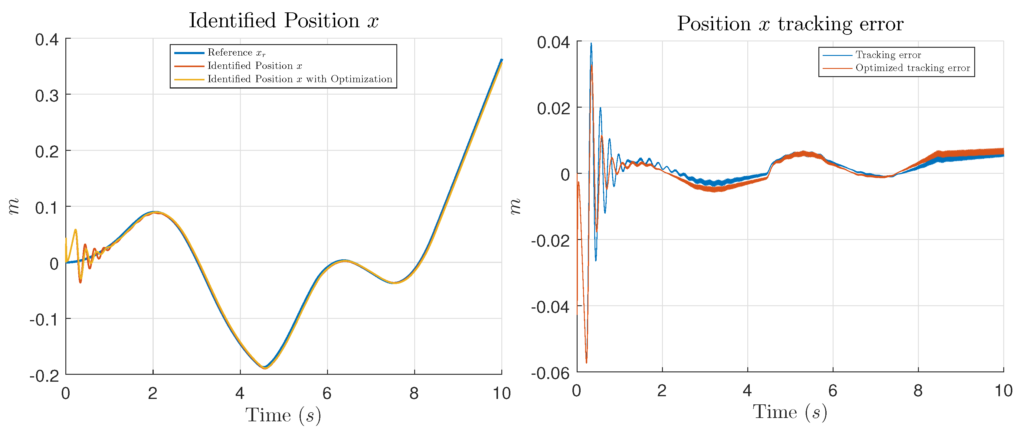
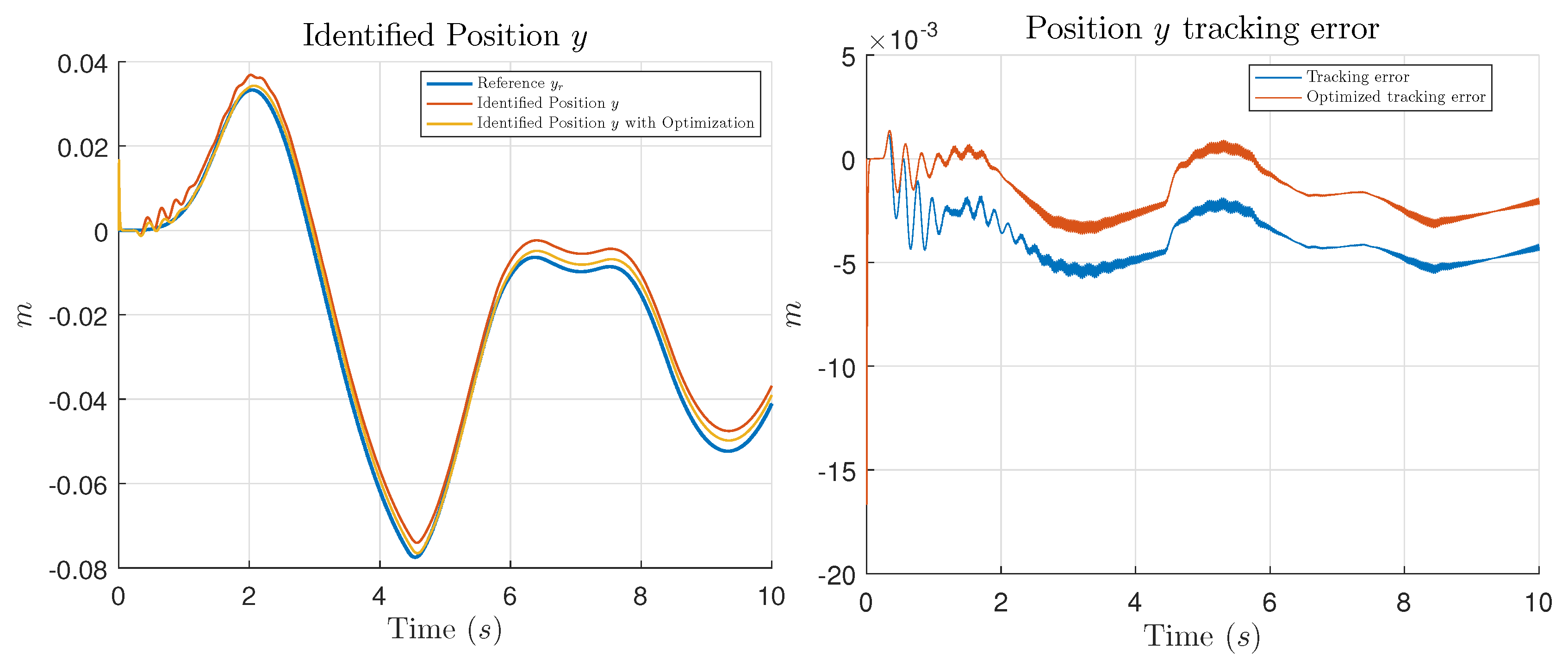
In this work, the main contribution is the introduction of an optimization process using GCO, in order to find the appropriate values for the controller parameters which minimize the tracking error of the system to be controlled. Performance of the optimization is shown presenting simulation and experimental tests comparing the results of the trajectory tracking using the NIOC with the parameters selected by the designer and the results using the parameters given by the GCO algorithm.

This work is organized as follows: In Section 2 the Germinal Center Optimization algorithm is described. In Section 2.1 the vertebrates adaptive immune system is briefly explained, in Section 2.2 we detail the germinal center reaction and in Section 2.3 the computation analogy of the germinal center reaction is presented along with the algorithm description. Section 3 introduces the Neural Inverse Optimal Control (NIOC) scheme for this work, where Section 3.1 presents the RHONN identifier and the extended kalman filter (EKF) training, and in Section 3.1.2 the design of the inverse optimal control law is discussed. 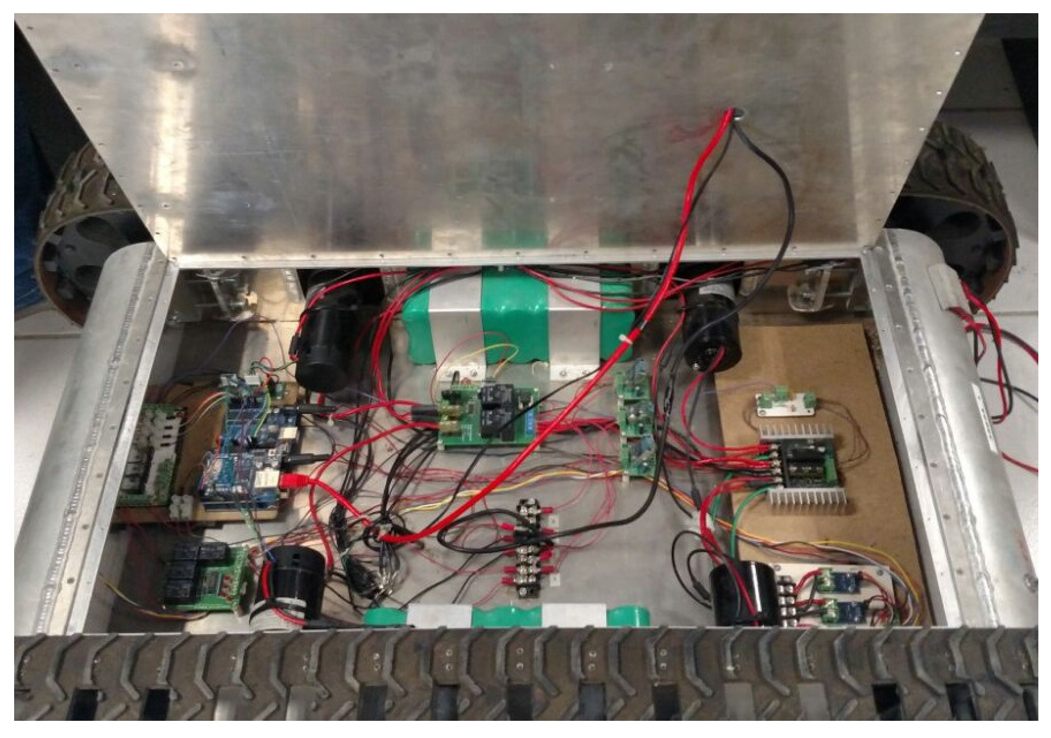Section 4 unveils comparative simulations (Section 4.2) and experimental (Section 4.3) results between the selection of the parameter of the controller using the GCO algorithm and the classic way which is let completely to the designer for an application of the NIOC to an All-Terrain Tracked Robot. Conclusions of this work are included in Section 5.

2. Germinal Center Optimization

In this section, we briefly overview the principal processes in the vertebrates immune system, and we detail the germinal center reaction. After that, we propose the computational analogy for multi-variate optimization, with the proper algorithm description.

2.1. Adaptive Immune System

The vertebrates immune system (VIS) is the biological mechanism for protecting the body from AG. There are two types of immunities, the innate immunity, and the adaptive one. The innate immunity is conformed by epithelial barriers that prevent the entrance of AG, phagocytes that swallow AG, FDCs that capture antigen and lymphocytes NKs (Natural Killers) that destroy any non-self cell.

The innate immunity is an inheritable protection that has been developed through natural selection, but if a new type of AG gets inside the body could overcome this basic protections, in this case, the adaptive immunity takes place. The adaptive immunity is conformed by B-cells whose main functions are to internalize AG for presentation and generate ABs, Th-cells that give a life signal to high-affinity B-cells and cytotoxic T-cells that kills own cells that are already infected or kills carcinogenic cells [6].

The affinity of the innate immunity is not diverse because it is coded in the germinal line, in the other hand the adaptive immunity has a high-affinity diversity because the receptors are produced for somatic recombination and variate with somatic hyper-mutation [6,18].

There are two types of adaptive immune response, the humoral immunity, and the cellular immunity. The first one is based on ABs that travel in the bloodstream, attaching to every compatible particle. The B-cells compete for antigen internalization and presentation to the Th-cell, whose reward them with a life signal, then the B-cell proliferates by clonal expansion and differentiates into plasmatic cells, releasing higher affinity ABs in the bloodstream.

There are some AGs that infect the owner cells and hide inside them, these cells are destroyed by the cellular immunity with the cytotoxic T-cell. The adaptive immune response has the following features, as is shown in [6]:

• Specificity: Ensure to produce a specific AB for a specific AG
• Diversity: The immune system is capable of responding to a great variety of AGs
• Memory: Using memory B-cells, the immune system is capable of fighting repeated infections
• Clonal expansion: Increase the number of lymphocytes with high affinity of certain AGs
• Homeostasis: The immune system recover from an infection by itself
• No self-reactivity: The immune system does not attack the host body in the present of AGs

2.2. Germinal Center

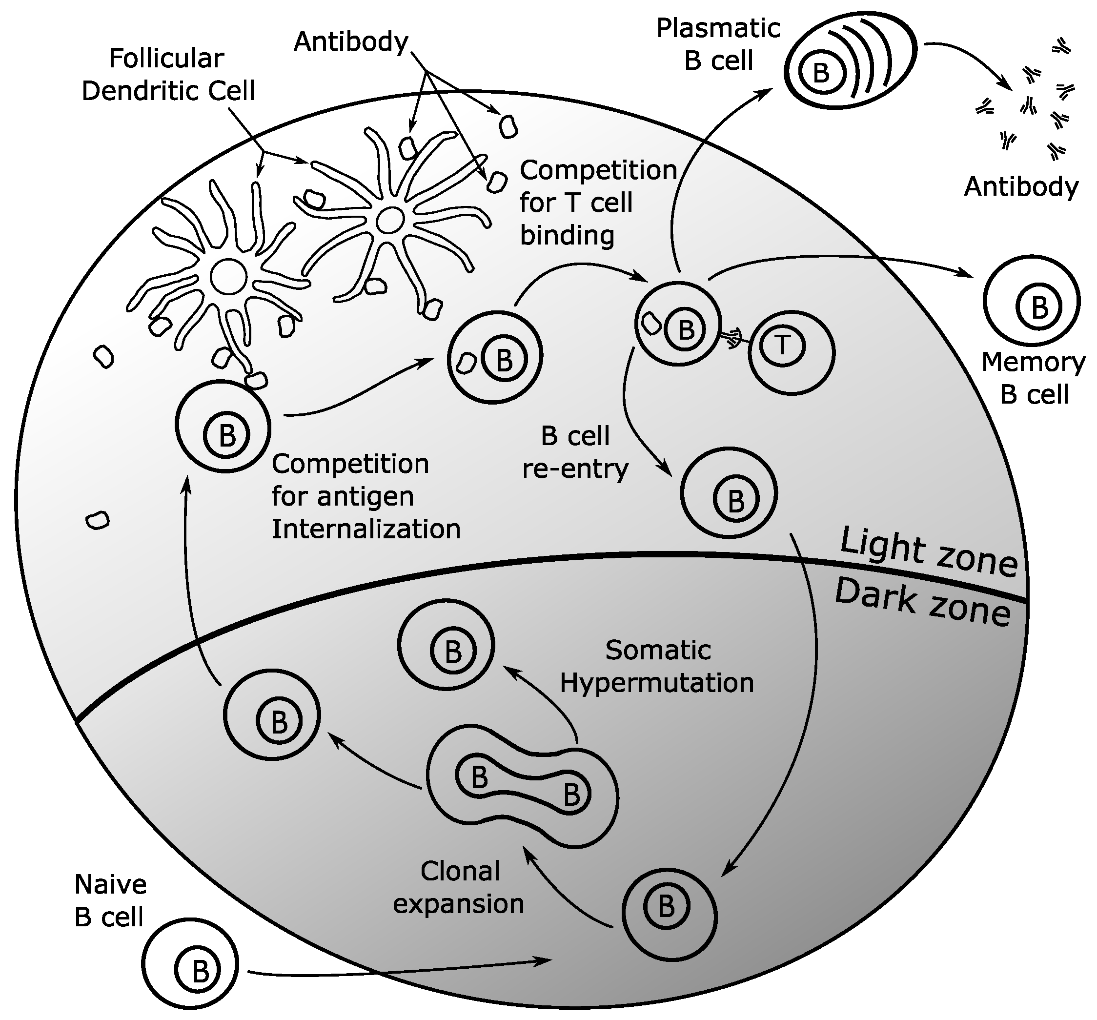
When the body does not have a specific AB for an infection, the body starts the process of affinity maturation with the germinal center reaction. Germinal centers are micro-anatomical regions in the secondary lymph nodes, that form in the present of antigen [10]. The AGs that survive the other immunity mechanism arrives at the secondary lymph nodes, where are capture for the FDCs. The FDCs activate near B-cells. The active B-cells end up being enclosed by the inactive ones forming a natural barrier that allow the active cells to proliferate, mutate and be selected.

The B-cells start to proliferate inside the GC, and compete for the antigen, this competition polarizes the GC in two distinct zones, the dark zone and the light zone. The dark zone is where B-cells proliferate through clonal expansion and somatic hyper-mutation, this process ensures the diversity of ABs. On the other hand, the light zone is where the B-cells are selected in accordance with their affinity.

On the light zone, the B-cells must find AG and internalize it, with the final purpose of digest the AG and expose their peptides to the Th-cell. The Th-cell gives a life signal allowing B-cells high affinity to live more time and therefore, proliferate and mutate with higher success.

In Figure 1, we show a schematic summary of the process. The GC reaction ensures the diversity through clonal expansion and somatic hyper-mutation in the dark zone, while in the light zone is a competitive process that reward the more adapted B-cells. The B-cells reentry to dark zone making this process an iterative refinement of the affinity [19,20].

Finally, when the GC generates high affinity B-cells for certain AG, some B-cells differentiate into plasmatic cells and release their ABs. A few B-cells become Memory B-cells that could live a long time and keeps information about this particular AG. Then, the GCs are capable of generating specific AB for a specific AG, and keep this information in Memory B-cells for future infections [21].

2.3. Algorithm Description

In this section, we explain the GCO algorithm. In

Table 1. Computational analogy between Germinal Center (GC) and Optimization.

Germinal Center	Optimization Problem
Antigen	Objective function
Antibody and B-cell	Candidate solution
Affinity	Objective function evaluation
T-help cell binding	Incrementation of life-signal

, we present the computational analogy between germinal center and the optimization problem.

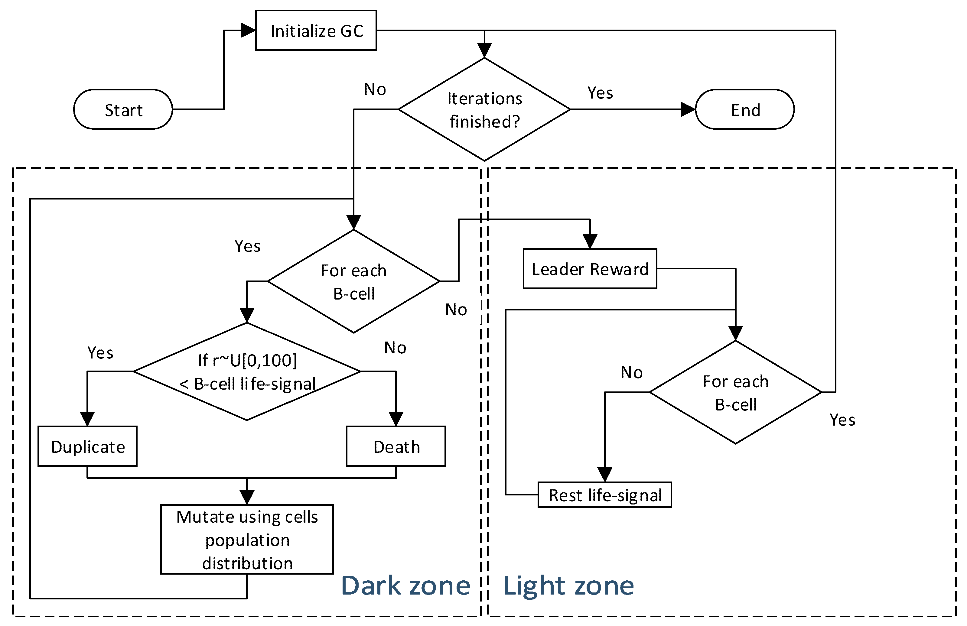
The GC reaction has multiple competitive processes, the GCO algorithm does not try to simulate GC reaction per se but to use some of its competitive mechanisms. A key factor in the GC reaction is the distinction between the dark zone and the light zone. The dark zone represents the diversification of the solutions that could be understood like a mutation process, many algorithms, such as Differential evolution and Genetic algorithms [1], already have the idea of mutation, but the dark zone includes not only a mutation process (somatic hyper-mutation), but also the clonal expansion. This clonal expansion is guided by the life signal of the B-cell, denoted by $\mathbb{L}\in [0,100]$. The B-cells with greater life signal are more likely to clone, increasing the B-cell multiplicity.

In the light zone, B-cells with the best affinity are rewarded and the other cells age (lower their life signal). Then, the affinity-based selection in the light zone changes the probability of clone or death of a B-cell. In Figure 2, we present the GCO algorithm flowchart, where “For each B-cell” indicates that the process is applied in every candidate solution.

As we are dealing with a population-based algorithm [1], there is a particular interest in the cells mutation and which information we use for crossover particles. In the GCO algorithm, we use the distribution of the cells multiplicity, denoted with $\mathcal{C}$, to select three individuals for crossover. It is important to note that initially, all the cells have a multiplicity of one, then the individuals are uniformly selected, but this distribution changes through iterations modeled by the competitive process. This kind of distribution offers different types of leadership behaviors in the collective intelligence, for example, initially the GCO algorithm behaves like Differential Evolution in the DE/rand/1 strategy [1], and when a particle wins for many iterations, the algorithm behaves like Particle Swarm optimization [1]. However, the leadership in GCO is not only dynamic, but it also includes temporal leadership, this is implemented when a particle mutates to a better solution, this new candidate substitutes the actual particle resetting the cell multiplicity to one.

Then, GCO algorithm offers a bio-inspired technique of adaptive leadership in collective intelligence algorithms for multivariate optimization problems. In Algorithm 1, we include an explicit pseudocode, where $B_i$ is the i-esim B-cell, M is a mutant B-cell and a new candidate solution, $F\in [0,2]$ is the mutation factor and $CR\in [0,1]$ is the cross-ratio, $\mathcal{C}$ is the distribution of cells multiplicity, and $\mathbb{L}$ is the life signal.

Algorithm 1: GCO algorithm

3. Neural Inverse Optimal Control

In this section, we introduced the neural identifier based on a RHONN and its EKF training, and the inverse optimal control law designed. Consider the following affine discrete-time nonlinear system

$$\begin{array}{c}\hfill \mathbf{x}\left(k\right)=f\left(\mathbf{x}\right(k)+g(\mathbf{x}\left(k\right)\left)\mathbf{u}\right(k)\end{array}$$

(1)

where $\mathbf{x}\in {\Re }^n$ is the state vector of the system, $\mathbf{u}\in {\Re }^m$ is the control input vector, $f\in {\Re }^n\to {\Re }^n$ and $g\in {\Re }^n\to {\Re }^{n\times m}$ are smooth maps.

3.1. Neural Identification with Recurrent High Order Neural Networks (RHONN)

To identify the system (1), we used the following RHONN identifier based on a RHONN in series-parallel model:

$$\begin{array}{ccc}\hfill {\widehat{\chi }}_i(k+1)& =& {\mathit{\omega }}_i^{\top }\left(k\right){\mathbf{z}}_i(\mathbf{x}(k-l),\mathbf{u}\left(k\right))\hfill \\ \hfill i& =& 1,2,\cdots ,n\hfill \end{array}$$

(2)

with

$$\begin{array}{c}\hfill {\mathbf{z}}_i(\mathbf{x}\left(k\right),\mathbf{u}\left(k\right))=\left[\begin{array}{c}{z}_{i_1}\\ z_{i_2}\\ ⋮\\ z_{i_{L_i}}\end{array}\right]=\left[\begin{array}{c}{\Pi }_{j\in I_1}{\mathit{\xi }}_{i_j}^{{d_i}_j\left(1\right)}\\ {\Pi }_{j\in I_2}{\mathit{\xi }}_{i_j}^{{d_i}_j\left(2\right)}\\ ⋮\\ {\Pi }_{j\in I_{L_i}}{\mathit{\xi }}_{i_j}^{{d_i}_j\left(L_i\right)}\end{array}\right],{\mathit{\xi }}_i=\left[\begin{array}{c}{\xi }_{i_1}\\ ⋮\\ {\xi }_{i_n}\\ {\xi }_{i_{n+1}}\\ ⋮\\ {\xi }_{i_{n+m}}\end{array}\right]=\left[\begin{array}{c}S\left(x_1(k-l)\right)\\ ⋮\\ S\left(x_n(k-l)\right)\\ u_1\left(k\right)\\ ⋮\\ u_m\left(k\right)\end{array}\right]\end{array}$$

(3)

where $S\left(v\right)=1/(1+exp(-\beta v\left)\right)$, $\beta >0$, n is the state dimension, $\widehat{\chi }$ is state vector of the neural network, $\mathit{\omega }$ is the weight vector $\mathbf{x}$ is the plant state vector, and $\mathbf{u}={[u_1,u_2,\dots ,u_m]}^{\top }$ is the input vector to the neural network.

The neural identifier (2) is presented in [14]. This neural identifier does not need previous knowledge of the model of the system, also, it does not need information of the disturbances and delays. Moreover, this model is semi-globally uniformly ultimately bounded (SGUUB) and the proof can be found in [14].

3.1.1. Training of RHONN with Extended Kalman Filter

The extended kalman filter estimates the state of a system with additive white noise in the input and in the output using a recursive solution in which each update of the state is estimated from the previous estimated state and the new input data [11,22].

For the case of neural networks the extended kalman filter training goal is to find the optimal weight vector which minimizes the prediction error. Due to the fact that the neural network mapping is non-lineal the extended kalman filter (EKF) is required. The EKF-based training algorithm [11] is (4):

$$\begin{array}{ccc}\hfill {\mathit{\omega }}_i(k+1)& =& {\mathit{\omega }}_i\left(k\right)+{\eta }_i{\mathbf{K}}_i\left(k\right)e_i\left(k\right)\hfill \end{array}$$

(4)

$$\begin{array}{ccc}\hfill {\mathbf{K}}_i\left(k\right)& =& {\mathbf{P}}_i\left(k\right){\mathbf{H}}_i\left(k\right){[R_i\left(k\right)+{\mathbf{H}}_i^{\top }\left(k\right){\mathbf{P}}_i\left(k\right){\mathbf{H}}_i\left(k\right)]}^{-1}\hfill \end{array}$$

(5)

$$\begin{array}{ccc}\hfill {\mathbf{P}}_i(k+1)& =& {\mathbf{P}}_i\left(k\right)-{\mathbf{K}}_i\left(k\right){\mathbf{H}}_i^{\top }\left(k\right){\mathbf{P}}_i\left(k\right)+{\mathbf{Q}}_i\left(k\right)\hfill \end{array}$$

(6)

with

$$e_i\left(k\right)=x_i\left(k\right)-{\widehat{\chi }}_i\left(k\right)$$

(7)

$$H_{ij}={\left[\frac{\partial {\widehat{\chi }}_i\left(k\right)}{\partial {\omega }_{ij}\left(k\right)}\right]}^{\top }$$

(8)

where $i=1\cdots n$, ${\mathit{\omega }}_i\in {\Re }^{L_i}$ is the on-line adapted weight vector, ${\mathbf{K}}_i\in {\Re }^{L_i}$ is the Kalman gain vector, $e_i\in \Re$ is the identification error, ${\mathbf{P}}_i\in {\Re }^{L_i\times L_i}$ is the weight estimation error covariance matrix, ${\chi }_i$ is the i-th state variable of the neural network, ${\mathbf{Q}}_i\in {\Re }^{L_i\times L_i}$ is the estimation noise covariance matrix, $R_i\in \Re$ is the error noise covariance matrix and ${\mathbf{H}}_i\in {\Re }^{L_i}$ is a vector in which each entry $H_{ij}$ is the derivative of the neural network state $\left({\widehat{\chi }}_i\right)$ with respect to one neural network weight $\left({\omega }_{ij}\right)$ and it is given by (8). ${\mathbf{P}}_i$ and ${\mathbf{Q}}_i$ are initialized as diagonal matrices with entries ${\mathbf{P}}_i\left(0\right)$ and ${\mathbf{Q}}_i\left(0\right)$, respectively. It is important to remark that ${\mathbf{H}}_i\left(k\right)$, ${\mathbf{K}}_i\left(k\right)$ and ${\mathbf{P}}_i\left(k\right)$ for the EKF are bounded.

3.1.2. Inverse Optimal Control

Optimal control finds a control law for a system such that a performance criterion is minimized. The criterion is a cost functional based on the state and control variables. The solution of the optimal control leads to the HJB equation which solution is not an easy task. Inverse optimal control is an alternative to optimal control, avoiding the HJB equation solution. For the inverse optimal control approach a stabilizing feedback control law based on a priori knowledge of a control Lyapunov function (CLF), is designed first, and then it is established that this control law optimizes a cost functional, then, the CLF is modified in order to achieve asymptotic tracking for given trajectory references [15]. The existence of a CLF implies stability and every CLF can be considered as a cost functional. The CLF approach for control synthesis has been applied successfully to systems for which a CLF can be established, such as feedback linearizable, strict feedback and feed-forward ones [15].

The system (1) is supposed to have an equilibrium point $\mathbf{x}\left(0\right)=\mathbf{0}$. Moreover, the full state $\mathbf{x}\left(k\right)$ is assumed to be available. In order to ensure stability of the system (1) the following control Lyapunov fuction is proposed:

$$V\left(\mathbf{x}\left(k\right)\right)=\frac{1}{2}\mathbf{x}{\left(k\right)}^{\top }\mathbf{P}\mathbf{x}\left(k\right),\mathbf{P}={\mathbf{P}}^{\top }>0$$

(9)

The inverse optimal control law for the system (1) with (9) is:

$$\begin{array}{ccc}\hfill \mathbf{u}\left(k\right)& =& -\frac{1}{2}{\mathbf{R}}^{-1}\left(\mathbf{x}\left(k\right)\right)g^{\top }\left(\mathbf{x}\left(k\right)\right)\frac{\partial V\left(\mathbf{x}\right(k\left)\right)}{\partial \mathbf{x}(k+1)}\hfill \\ & =& -\frac{1}{2}{(\mathbf{R}\left(\mathbf{x}\left(k\right)\right)+\frac{1}{2}{g}^{\top }\left(\mathbf{x}\left(k\right)\right)\mathbf{P}g\left(\mathbf{x}\left(k\right)\right))}^{-1}{g}^{\top }\left(\mathbf{x}\left(k\right)\right)\mathbf{P}f\left(\mathbf{x}\left(k\right)\right)\hfill \end{array}$$

(10)

where $\mathbf{R}\left(\mathbf{x}\left(k\right)\right)=\mathbf{R}{\left(\mathbf{x}\left(k\right)\right)}^{\top }>\mathbf{0}$ is a matrix whose elements can be functions of the system state or can be fixed. $\mathrm{P}$ is a matrix such that the inequality (11) holds.

$$\begin{array}{c}{V}_f\left(\mathbf{x}\left(k\right)\right)-\frac{1}{4}{\mathbf{P}}_1^{\top }\left(\mathbf{x}\left(k\right)\right){\left(\mathbf{RP}\left(\mathbf{x}\left(k\right)\right)\right)}^{-1}{\mathbf{P}}_1\left(\mathbf{x}\left(k\right)\right)\le -{\mathbf{x}}^{\top }\left(k\right)\mathbf{Q}\mathbf{x}\left(k\right)\hfill \end{array}$$

(11)

with

$$\begin{array}{ccc}\hfill \mathbf{RP}\left(\mathbf{x}\right(k\left)\right)& =& \mathbf{R}\left(\mathbf{x}\left(k\right)\right)+{\mathbf{P}}_2\left(\mathbf{x}\left(k\right)\right)\hfill \end{array}$$

(12)

$$\begin{array}{ccc}\hfill V_f\left(\mathbf{x}\left(k\right)\right)& =& \frac{1}{2}{f}^{\top }\left(\mathbf{x}\left(k\right)\right)\mathbf{P}f\left(\mathbf{x}\left(k\right)\right)-V\left(\mathbf{x}\left(k\right)\right)\hfill \end{array}$$

(13)

$$\begin{array}{ccc}\hfill {\mathbf{P}}_1\left(\mathbf{x}\left(k\right)\right)& =& g^{\top }\left(\mathbf{x}\left(k\right)\right)\mathbf{P}f\left(\mathbf{x}\left(k\right)\right)\hfill \end{array}$$

(14)

$$\begin{array}{ccc}\hfill {\mathbf{P}}_2\left(\mathbf{x}\left(k\right)\right)& =& \frac{1}{2}{g}^{\top }\left(\mathbf{x}\left(k\right)\right)\mathbf{P}g\left(\mathbf{x}\left(k\right)\right)\hfill \end{array}$$

(15)

$$\begin{array}{ccc}\hfill \mathbf{Q}& =& {\mathbf{Q}}^{\top }>0\hfill \end{array}$$

(16)

In [15], it is demonstrated that control law (10) is globally asymptotically stable. Moreover, (10) is inverse optimal in the sense that minimizes a cost functional [15].

4. Results

In this section, we briefly describe how GCO is applied to improve NIOC performance, we also show simulation results and real-time experimental results. The all-terrain tracked robot is a modified HD2^® (HD2 is a registered trademark of SuperDroid Robots), shown in Figure 3. The changes of the modified HD2^® are (Figure 4): the replacement of the original board for a system based on Arduino^® (Arduino is a registered trademark of Arduino LLC), and an attachment of a wireless router. Chassis, tracks, batteries, and motors remained without modifications.

4.1. Application to All-Terrain Tracked Robot Control

Considered as the most important type of mobile robots, a tracked robot runs on continuous tracks instead of wheels which develop a thrust higher than a wheeled robot. This kind of robots is ideal for working in tasks under rough terrains. Among the applications tracked robots can achieve are urban reconnaissance, forestry, mining, agriculture, rescue mission scenarios, autonomous planetary explorations [23,24,25].

A tracked robot consists of the following state variables [17,26,27] position x, position y, position $\theta$, velocity 1, velocity 2, current 1 and current 2. In this work, we focus on the controller tracking performance for x, y and $\theta$ (Figure 5) for given references $x_r$, $y_r$ and ${\theta }_r$. The objective is to improve the NIOC results presented in [17] by using GCO to find the optimal parameters of the controller. These parameters are included in the matrices ${\mathbf{P}}_1$ and ${\mathbf{P}}_2$ defined in (11) and (12) respectively. The ${\mathbf{P}}_1$ and ${\mathbf{P}}_2$ are symmetric positive definite matrices, therefore we can define the set of variables $\{{\psi }_1,{\psi }_2,{\psi }_3,{\psi }_4,{\psi }_5\}$ for the optimization problem with the definition in (17).

$${\mathbf{P}}_1=\left[\begin{array}{ccc}{\psi }_1& {\psi }_2& {\psi }_3\\ {\psi }_2& {\psi }_1& {\psi }_4\\ {\psi }_3& {\psi }_4& {\psi }_1\end{array}\right]{\mathbf{P}}_2=\left[\begin{array}{cc}{\psi }_5& 0\\ 0& {\psi }_5\end{array}\right]$$

(17)

The lower bound of the search space is given by $\{1,1,1,1,1\}$ and the upper bound is given by $\{4\times {10}^7,4\times {10}^7,4\times {10}^7,4\times {10}^7,4\times {10}^4\}$. Next, the objective of the optimization is to get a better control tracking, in order to achieve this, we minimize the sum of the Root Mean Square Error (RMSE) in every state. This idea is described by (18), where n is the number of samples of the reference and estimated functions, we are using $n=3335$ for real-time experiments and $n=5000$ for simulation experiments.

$$f=\underset{{\psi }_1,{\psi }_2,{\psi }_3,{\psi }_4,{\psi }_5}{min}\sqrt{\frac{{\sum }_{i=1}^n{(\widehat{x}-x)}^2}{n}}+\sqrt{\frac{{\sum }_{i=1}^n{(\widehat{y}-y)}^2}{n}}+\sqrt{\frac{{\sum }_{i=1}^n{(\widehat{\theta }-\theta )}^2}{n}}$$

(18)

Then, the GCO algorithm will find optimal values that minimize (18). For the following experiments we use a GCO algorithm in five dimension running 150 iterations using 30 B-cells (4500 executions) for a test of 10 seconds; we set the parameters $F=1.25$ and $CR=0.7$. We include graphics for one simulation test using the all-terrain robot model presented in [17], and the results of one experimental test using the modified HD2^® Treaded ATR Tank Robot Platform with wireless communication (Figure 3) presented in [17].

4.2. Simulation Results

In [17], ${\mathbf{P}}_1$ and ${\mathbf{P}}_2$ are defined as shown in (19) for simulation. We show in (20) ${\mathbf{P}}_1^{*}$ and ${\mathbf{P}}_2^{*}$, which contain the parameters found by the GCO algorithm.

$${\mathbf{P}}_1=14400\left[\begin{array}{ccc}162& 1& 2\\ 1& 162& 3\\ 2& 3& 162\end{array}\right]{\mathbf{P}}_2=20\left[\begin{array}{cc}20& 0\\ 0& 20\end{array}\right]$$

(19)

$${\mathbf{P}}_1^{*}=1\times {10}^6\left[\begin{array}{ccc}5.7564& 0& 0\\ 0& 5.7564& 0\\ 0& 0& 5.7564\end{array}\right]{\mathbf{P}}_2^{*}=\left[\begin{array}{cc}40000& 0\\ 0& 40000\end{array}\right]$$

(20)

Figure 6, Figure 7 and Figure 8 show the tracking performance and the error comparison for the position x, position y and position $\theta$ of the simulation test. For each figure, the graph on the left side shows the obtained signals for reference, the identified signal using NIOC [17], and the identified signal using the optimized NIOC for its respective state variable. The graph on the right side shows the obtained the error signals for the NIOC [17] and the optimized NIOC for its respective state variable. This arrangement is maintained for all the following figures in this section.

Table 2. Root Mean Squared Error (RMSE) in states for second simulation. Bold values highlight the best result.

Control	RMSE x (m)	RMSE y (m)	RMSE $\mathit{\theta }$ (rad)	Total
NIOC [17]	0.0073	0.0043	0.0064	0.0180
NIOC with GCO	0.0073	0.0025	0.0049	0.0147

shows the RMSE of each state variable and their total which is the evaluation of Equation (18) for this simulation test. Total does not have a physical meaning, it is the minimum found in the objective function in (18).

A second simulation test was made resulting in the tracking errors shown in

Table 3. Root Mean Squared Error (RMSE) in states for first simulation. Bold values highlight the best result.

Control	RMSE x (m)	RMSE y (m)	RMSE $\mathit{\theta }$ (rad)	Total
NIOC [17]	0.0077	0.0055	0.0064	0.0195
NIOC with GCO	0.0079	0.0041	0.0049	0.0169

.

Additionally to the presented results, in [17] it was demonstrated via simulations that the NIOC has a better performance than a super twisting scheme for a tracked robot model. The tracking comparison results shown in

Table 4. Tracking error comparison of NIOC [17] and a Super Twisting controller. Bold values highlight the best result.

RMSE	x (m)	y (m)	$\mathit{\theta }$ (rad)
NIOC [17]	0.0260	0.0362	0.0158
Super Twisting	0.0317	0.0036	0.0652

are reported in [17].

4.3. Real-Time Results

The work [17] presents a NOIC for the Modified HD2^® Treaded ATR Tank Robot Platform with wireless communication (Figure 3), this implementation uses an RHONN identifier as (2) to identify the unknown model of the HD2^®. The obtained model is then used as the based to synthesize the control law using the inverse optimal control approach. In [17] the values of ${\mathbf{P}}_1$ and ${\mathbf{P}}_2$ are defined in (21) for real-time operation. The following results show a comparison obtained with the values from [17] and ${\mathbf{P}}_1^{*}$ and ${\mathbf{P}}_2^{*}$ in (22) found by the GCO algorithm. In this section, there are presented two experiments named as “test 1” and “test 2”, respectively.

$${\mathbf{P}}_1=72000\left[\begin{array}{ccc}162& 1& 2\\ 1& 162& 3\\ 2& 3& 162\end{array}\right]{\mathbf{P}}_2=10000\left[\begin{array}{cc}20& 0\\ 0& 20\end{array}\right]$$

(21)

$${\mathbf{P}}_1^{*}=1\times {10}^7\left[\begin{array}{ccc}3.2039& 0& 4\\ 0& 3.2039& 0\\ 4& 0& 3.2039\end{array}\right]{\mathbf{P}}_2^{*}=1\times {10}^4\left[\begin{array}{cc}2.4128& 0\\ 0& 2.4128\end{array}\right]$$

(22)

Figure 9, Figure 10 and Figure 11 show the tracking performance and the error comparison for the position x, position y and position $\theta$ of the experimental test 1.

Table 5. Root Mean Squared Error in states for Real-Time experimental test 1. Bold values highlight the best result.

Control	RMSE x (m)	RMSE y (m)	RMSE $\mathit{\theta }$ (rad)	Total
NIOC [17]	0.0238	0.0109	0.0267	0.0614
NIOC with GCO	0.0152	0.0043	0.0270	0.0465

shows the RMSE of each state variable and their total which is the evaluation of Equation (18) for the experimental test 1.

Figure 12, Figure 13 and Figure 14 show the tracking performance and the error comparison for the position x, position y and position $\theta$ of the experimental test 2.

Table 6. Root Mean Squared Error (RMSE) in states for Real-Time experimental test 2. Bold values highlight the best result.

Control	RMSE x (m)	RMSE y (m)	RMSE $\mathit{\theta }$ (rad)	Total
NIOC [17]	0.0153	0.0052	0.0101	0.0305
NIOC with GCO	0.0100	0.0021	0.0123	0.0244

shows the RMSE of each state variable and their total which is the evaluation of Equation (18) for the experimental test 2.

5. Conclusions

GCO is a hybridization between Evolutionary Computing and Artificial Immune System based on the Germinal Center reaction which is a biological process in vertebrates immune system that maturates affinity of antibodies. GCO models a population of B-cells and the competitive process in their proliferation, then, a dynamic distribution of the cells multiplicity is constructed over the performance of the candidate solutions. This distribution allows to select B-cells for crossover with an adaptive leadership. The adaptive leadership takes the advantage of both high leadership and none leadership algorithms allowing it to find a better solution.

In this work, it is shown how GCO can help with the overall performance of a control technique like inverse optimal control, which depends on a number of designed parameters. Our results reveal a better performance of the controller version with the parameters obtained with GCO. It is also important to mention that the found parameters by GCO for the NIOC are not unique for a reference, those parameters can work for a number of references.

References

1. Simon, D. Evolutionary Optimization Algorithms; John Wiley & Sons: Hoboken, NJ, USA, 2013. [Google Scholar]
2. Haykin, S. Neural Networks and Learning Machines; Prentice Hall: Upper Saddle River, NJ, USA, 2009. [Google Scholar]
3. Brabazon, A.; O’Neill, M.; McGarraghy, S. Artificial Immune Systems. In Natural Computing Algorithms; Springer: Berlin, Germany, 2015; pp. 301–332. [Google Scholar]
4. Dasgupta, D.; Yu, S.; Nino, F. Recent advances in artificial immune systems: Models and applications. Appl. Soft Comput. 2011, 11, 1574–1587. [Google Scholar] [CrossRef]
5. Timmis, J.; Hone, A.; Stibor, T.; Clark, E. Theoretical advances in artificial immune systems. Theor. Comput. Sci. 2008, 403, 11–32. [Google Scholar] [CrossRef]
6. Abbas, A.K.; Lichtman, A.H.; Pillai, S. Cellular and Molecular Immunology; Elsevier Health Sciences: Amsterdam, The Netherlands, 2014. [Google Scholar]
7. Ulutas, B.H.; Kulturel-Konak, S. A review of clonal selection algorithm and its applications. Artif. Intell. Rev. 2011, 36, 117–138. [Google Scholar] [CrossRef]
8. Dai, H.; Yang, Y.; Li, H.; Li, C. Bi-direction quantum crossover-based clonal selection algorithm and its applications. Expert Syst. Appl. 2014, 41, 7248–7258. [Google Scholar] [CrossRef]
9. Gao, S.; Dai, H.; Zhang, J.; Tang, Z. An expanded lateral interactive clonal selection algorithm and its application. IEICE Trans. Fundam. Electron. Commun. Comput. Sci. 2008, 91, 2223–2231. [Google Scholar] [CrossRef]
10. Victora, G.D.; Nussenzweig, M.C. Germinal centers. Ann. Rev. Immunol. 2012, 30, 429–457. [Google Scholar] [CrossRef] [PubMed]
11. Sanchez, E.N.; Alanis, A.Y.; Loukianov, A.G. Discrete-Time High Order Neural Control: Trained with Kalman Filtering; Springer: Berlin, Germany, 2008. [Google Scholar]
12. Alanis, A.; Sanchez, E. Discrete-Time Neural Observers: Analysis and Applications; Elsevier Science: Amsterdam, The Netherlands, 2017. [Google Scholar]
13. Zhang, M. Artificial Higher Order Neural Networks for Economics and Business; IGI Global Research Collection, Information Science Reference: Hershey, PA, USA, 2008. [Google Scholar]
14. Alanis, A.Y.; Rios, J.D.; Arana-Daniel, N.; Lopez-Franco, C. Neural identifier for unknown discrete-time nonlinear delayed systems. Neural Comput. Appl. 2016, 27, 2453–2464. [Google Scholar] [CrossRef]
15. Sanchez, E.; Ornelas-Tellez, F. Discrete-Time Inverse Optimal Control for Nonlinear Systems; EBL-Schweitzer, CRC Press: Boca Raton, FL, USA, 2016. [Google Scholar]
16. Lopez, V.G.; Sanchez, E.N.; Alanis, A.Y.; Rios, J.D. Real-time neural inverse optimal control for a linear induction motor. Int. J. Control 2017, 90, 800–812. [Google Scholar] [CrossRef]
17. Rios, J.D.; Alanis, A.Y.; Lopez-Franco, M.; Lopez-Franco, C.; Arana-Daniel, N. Real-time neural identification and inverse optimal control for a tracked robot. Adv. Mech. Eng. 2017, 9, 1687814017692970. [Google Scholar] [CrossRef]
18. Di Noia, J.M.; Neuberger, M.S. Molecular mechanisms of antibody somatic hypermutation. Annu. Rev. Biochem. 2007, 76, 1–22. [Google Scholar] [CrossRef] [PubMed]
19. Meyer-Hermann, M.; Mohr, E.; Pelletier, N.; Zhang, Y.; Victora, G.D.; Toellner, K.M. A theory of germinal center B cell selection, division, and exit. Cell Rep. 2012, 2, 162–174. [Google Scholar] [CrossRef] [PubMed]
20. Zhang, Y.; Meyer-Hermann, M.; George, L.A.; Figge, M.T.; Khan, M.; Goodall, M.; Young, S.P.; Reynolds, A.; Falciani, F.; Waisman, A.; et al. Germinal center B cells govern their own fate via antibody feedback. J. Exp. Med. 2013, 210, 457–464. [Google Scholar] [CrossRef] [PubMed]
21. Adachi, Y.; Onodera, T.; Yamada, Y.; Daio, R.; Tsuiji, M.; Inoue, T.; Kobayashi, K.; Kurosaki, T.; Ato, M.; Takahashi, Y. Distinct germinal center selection at local sites shapes memory B cell response to viral escape. J. Exp. Med. 2015, 212, 1709–1723. [Google Scholar] [CrossRef] [PubMed]
22. Haykin, S. Kalman Filtering and Neural Networks; Adaptive and Cognitive Dynamic Systems: Signal Processing, Learning, Communications and Control; Wiley: New York, NY, USA, 2004. [Google Scholar]
23. Wong, J.; Huang, W. “Wheels vs. tracks”—A fundamental evaluation from the traction perspective. J. Terramech. 2006, 43, 27–42. [Google Scholar] [CrossRef]
24. Siegwart, R.; Nourbakhsh, I.; Scaramuzza, D. Introduction to Autonomous Mobile Robots; Intelligent Robotics and Autonomous Agents; MIT Press: Cambridge, MA, USA, 2011. [Google Scholar]
25. González, R.; Rodríguez, F.; Guzmán, J. Autonomous Tracked Robots in Planar Off-Road Conditions: Modelling, Localization, and Motion Control; Springer: Berlin, Germany, 2014. [Google Scholar]
26. Das, T.; Kar, I.N. Design and implementation of an adaptive fuzzy logic-based controller for wheeled mobile robots. IEEE Trans. Control Syst. Technol. 2006, 14, 501–510. [Google Scholar] [CrossRef]
27. Moosavian, S.A.A.; Kalantari, A. Experimental slip estimation for exact kinematics modeling and control of a Tracked Mobile Robot. In Proceedings of the 2008 IEEE/RSJ International Conference on Intelligent Robots and Systems, Nice, France, 22–26 September 2008; pp. 95–100. [Google Scholar]
Figure 1. Germinal Center reaction.
Applsci 08 00031 g001
Figure 2. Germinal Center Optimization (GCO) algorithm flowchart.
Applsci 08 00031 g002
Figure 3. Modified HD2® Treaded All-Terrain Tracked Robot (ATR) Tank Robot Platform with wireless communication.
Applsci 08 00031 g003
Figure 4. The interior of the Modified HD2® Treaded ATR Tank Robot.
Applsci 08 00031 g004
Figure 5. Schematic representation of a tracked robot, where x and y are the coordinates of P 0 and θ is the heading angle.
Applsci 08 00031 g005
Figure 6. Tracking of x position (left) and error comparison (right) for the simulation test.
Applsci 08 00031 g006
Figure 7. Tracking of y position (left) and error comparison (right) for the simulation test.
Applsci 08 00031 g007
Figure 8. Tracking of θ (left) and error comparison (right) for the simulation test.
Applsci 08 00031 g008
Figure 9. Tracking of x position (left) and error comparison (right) for the experimental test 1.
Applsci 08 00031 g009
Figure 10. Tracking of y position (left) and error comparison (right) for the experimental test 1.
Applsci 08 00031 g010
Figure 11. Tracking of θ (left) and error comparison (right) for the experimental test 1.
Applsci 08 00031 g011
Figure 12. Tracking of x position (left) and error comparison (right) for the experimental test 2.
Applsci 08 00031 g012
Figure 13. Tracking of y position (left) and error comparison (right) for the experimental test 2.
Applsci 08 00031 g013
Figure 14. Tracking of θ (left) and error comparison (right) for the experimental test 2.
Applsci 08 00031 g014