A Synthetic Nervous System Controls a Simulated Cockroach

Department of Mechanical and Aerospace Engineering, Case Western Reserve University, Cleveland, OH 44106, USA
*
Author to whom correspondence should be addressed.
Appl. Sci. 2018, 8(1), 6; https://doi.org/10.3390/app8010006
Submission received: 14 November 2017
/
Revised: 19 December 2017
/
Accepted: 19 December 2017
/
Published: 22 December 2017
(This article belongs to the Special Issue Bio-Inspired Robotics)
Abstract
:The purpose of this work is to better understand how animals control locomotion. This knowledge can then be applied to neuromechanical design to produce more capable and adaptable robot locomotion. To test hypotheses about animal motor control, we model animals and their nervous systems with dynamical simulations, which we call synthetic nervous systems (SNS). However, one major challenge is picking parameter values that produce the intended dynamics. This paper presents a design process that solves this problem without the need for global optimization. We test this method by selecting parameter values for SimRoach2, a dynamical model of a cockroach. Each leg joint is actuated by an antagonistic pair of Hill muscles. A distributed SNS was designed based on pathways known to exist in insects, as well as hypothetical pathways that produced insect-like motion. Each joint’s controller was designed to function as a proportional-integral (PI) feedback loop and tuned with numerical optimization. Once tuned, SimRoach2 walks through a simulated environment, with several cockroach-like features. A model with such reliable low-level performance is necessary to investigate more sophisticated locomotion patterns in the future.
1. Introduction
Insects are excellent models for walking robots, for two reasons. First, insects are highly successful animals that can walk through a variety of terrains. Second, decades of behavioral and neurobiological research have revealed many of the neuromechanical mechanisms that underlie this adaptive behavior.
The legs of walking animals propel the body by alternating between stance and swing phases. A leg is in contact with the ground in stance phase, during which it supports and propels the body. A leg is not in contact with the ground in swing phase, during which it is returned from its position at the end of stance phase (posterior extreme position, or PEP) to its position at the beginning of stance phase (anterior extreme position, or AEP). This alternating activity is supported by central pattern generators (CPGs), networks that are capable of producing endogenous oscillatory output. Each leg joint appears to be controlled by its own CPG [1,2]. Although periods of coordinated behavior can be observed [3], each leg joint’s activity is generally decoupled from that of the others [2]. CPGs’ phases are adjusted by inter-joint signals from load [4,5,6] and proprioceptive [7,8] sensors, giving rise to the coordination seen during walking. When walking in different directions, some of these inter-joint reflexes are modified [9,10], giving rise to different coordination patterns that better serve locomotion in a particular direction. Indeed, stimulating populations in the insect central complex (CX) that encode locomotion direction can change the sign and phase of inter-joint reflexes as observed in intact animals [11].
There is an interdependent relationship between neuroscience, mathematical modeling, and robotics. The neuroscience of insects promises to inspire new and adaptive robot control systems (for a review, see [12]). However, mathematical modeling of the nervous system and the body’s mechanics is often a necessary intermediate step between neuroscience and robotics. First, despite decades of wonderful work, there still exist many gaps in our understanding of how insects walk. Thus, a mathematical model can be constructed that incorporates what is known, and suggests how to bridge gaps in understanding [13,14]. Second, it is valuable to test the control method first in a simulated agent before controlling a robot. This enables a more thorough study of the function and stability of the system in a simplified environment before deploying it on a hardware system in the real world.
Many models exist to address specific questions about motor control in insects. Walknet, for example, has developed into a highly successful model. It uses a combination of finite state machine (FSM) and artificial neural network (ANN) elements to coordinate the walking of kinematic models [15] and hardware robots [16]. While Walknet is a capable walking controller, it is based on behavioral, not neurobiological data, making it difficult to test neurobiological hypotheses. Another model used similar FSM elements to demonstrate how decoupled CPGs could be coordinated into stepping motions via sensory feedback [17]. This model was even used to control a single robotic leg [18]. These works were important proofs of concept for the control of a leg via sensory-coupled CPGs. However, the simplicity of the model made it difficult to produce fine-tuned motions necessary for walking. In addition, the FSM implementation leaves out the details of neural dynamics, which can produce more complicated and potentially more capable motor patterns. More recently, Hodgkin–Huxley neural models of networks in insect nervous systems have been constructed to explore the effect of such neural dynamics on locomotion [13,19,20,21]. These models have enabled scientists to suggest neural and synaptic mechanisms underlying animal behavior. However, due to their complexity, the full mechanics of the body and environment are rarely simulated, leaving questions about the precise control of muscle activation, and the role of sensory feedback, unaddressed.
Over the years, there has been much successful work building and controlling six-legged robots [15,16,22,23,24]. However, despite all of this good work, these robots are not as good at locomotion as insects. We believe that an SNS will result in better performance.
To be directly applicable to robotic control, the mechanical model must possess realistic dynamics, and the neural system must use feedback from interactions with the environment to shape motor output.
Our recent work has explored many components of legged locomotion, although always limited to one leg. We have shown how a decoupled system of central pattern generators (CPGs) can give rise to directional stepping with only sparse descending commands [25]. This control approach can be applied to different legs, resulting in unique motions for each leg, as observed in walking insects [14,26,27,28]. However, adding more legs to the body makes walking a redundant problem, with several paths from body to ground. Successful locomotion requires controlling both the timing and amplitude of motor output to ensure that the body remains supported at all times [29].
This work expands upon our previous model of insect locomotion [14] and presents three novel results. The first is the development of a generalized design method for setting parameters in neuromechanical models. The control method uses the dynamics of the body to establish a resting posture, set passive viscoelastic forces based on the scale of the model, and set parameters in a negative feedback position controller for the antagonistic pair of muscles that actuate each leg joint. The result is a model with realistic dynamics, and accurate control of the leg joints. The second result is a neural implementation of “Holk Cruse’s rules” [29], which precisely and stably controls the timing of each leg’s swing phase. The third result is the comparison between biological and simulated walking data. The resulting model can walk freely at cockroach-like speed and stepping frequency. Such performance supports the usefulness of the presented design method. This model serves as a baseline for studying more complicated control problems in the future, such as walking in a curve, walking at different speeds, and walking over rough terrain.
2. Methods
2.1. Modeling Overview
All modeling was done in AnimatLab 2, an environment for neuromechanical simulations [30]. The software can simulate the closed-loop interactions between an animat’s body, its nervous system, and and its environment. For example, motor neuron voltage affects the force in the muscles, which exert forces on the body to cause motion, which is detected by proprioceptors and force sensors, which affect motor neuron voltage.
Previously, we developed design tools in MATLAB (The MathWorks, Nattick, MA) to perform analysis to aid in the parameter value design process. Versions of these tools existed previously [26,31], but these tools had to be advanced significantly to incorporate additional dynamics due to muscles and exoskeletal forces. This work thus extends tools previously only useful for robots controlled by servomotors to animal models like SimRoach2, which was developed in this project.
2.2. System Dynamics
2.2.1. Neuron Dynamics
A number of different mathematical models exist that attempt to capture the behavior of neurons. Our neural controller uses non-spiking Hodgkin–Huxley (HH) compartments [30], which are based on the original formulation of the HH model [32], but do not include ion channels for spiking. Thus the neurons function as non-spiking leaky integrators, with optional persistent sodium channels which enable more complicated responses. For details on the specific equations of motion, see the Supplementary Materials (Section: Methods Explained).
2.2.2. Muscle and Joint Dynamics
Each joint of SimRoach2 is actuated by two antagonistic Hill muscles [33]. This model contains an active contractile element, and three passive components: a series spring, a parallel spring, and a parallel damper (Figure 1). The primary dynamical variable for the muscle is its tension, T, with the dynamics:
where b is the linear damping coefficient, is the stiffness of the series elastic component, and is the stiffness of the parallel elastic component. is the change in muscle length relative to its resting length. is the rate of change of the muscle length. A is the muscle activation and is a function of both the muscle’s motor-neuron’s voltage and the length of the muscle. A is given by:
where is the width of the inverted parabola used for the tension-length curve and is a function of the motor-neurons voltage given by the sigmoid:
where , , , and are all parameters that define the stimulus-tension sigmoidal curve.
In addition to the two muscles acting on each joint, there is also a passive spring with damping attached to each joint to mimic the viscoelasticity of insects’ joints [35,36]. This stabilizes the motion of each joint, but makes the relationship between muscle activation and joint rotation more complicated. It shares attachments with the flexor muscle, and produces the tension:
where is the tension in the passive element, and are the stiffness and damping constants, respectively, is the resting length of the passive element, and x is the current length of the passive element.
When the leg is not in contact with the ground, there are four external moments acting on the joint: tensions from the flexor and extensor muscles, and spring stiffness and spring damping forces from the passive spring. The equation for the net torque on the joint can be developed as:
where is the moment arm of the force and corresponds to the flexor muscle force, corresponds to the extensor muscle force, corresponds to the linear spring stiffness force, and corresponds to the linear spring damping force.
2.3. Physical Model
SimRoach2 (Figure 2) was adapted from our previous model [14]. Each leg has five actuated hinge joints (Table 1). Each foot is modeled as a passive ball and socket joint that “sticks” to the ground in stance phase but allows the tibia to rotate over the foot. This functionality mimics insects’ tarsal claws, which grip the substrate when external forces are applied [37], and can improve the stability of walking [38]. Furthermore, it has been shown that the adhesive features on an insect’s leg plays an important role in walking [39]. Thus, the animat’s body has 54 degrees of freedom (), 30 of which are actuated, and 6 of which are constrained for each leg when it is in contact with the ground. See Figure 4 in [14] for a description of the different body segments and joint angles in a cockroach.
2.4. Neural Network as Control System
2.4.1. Overview of Synthetic Nervous System
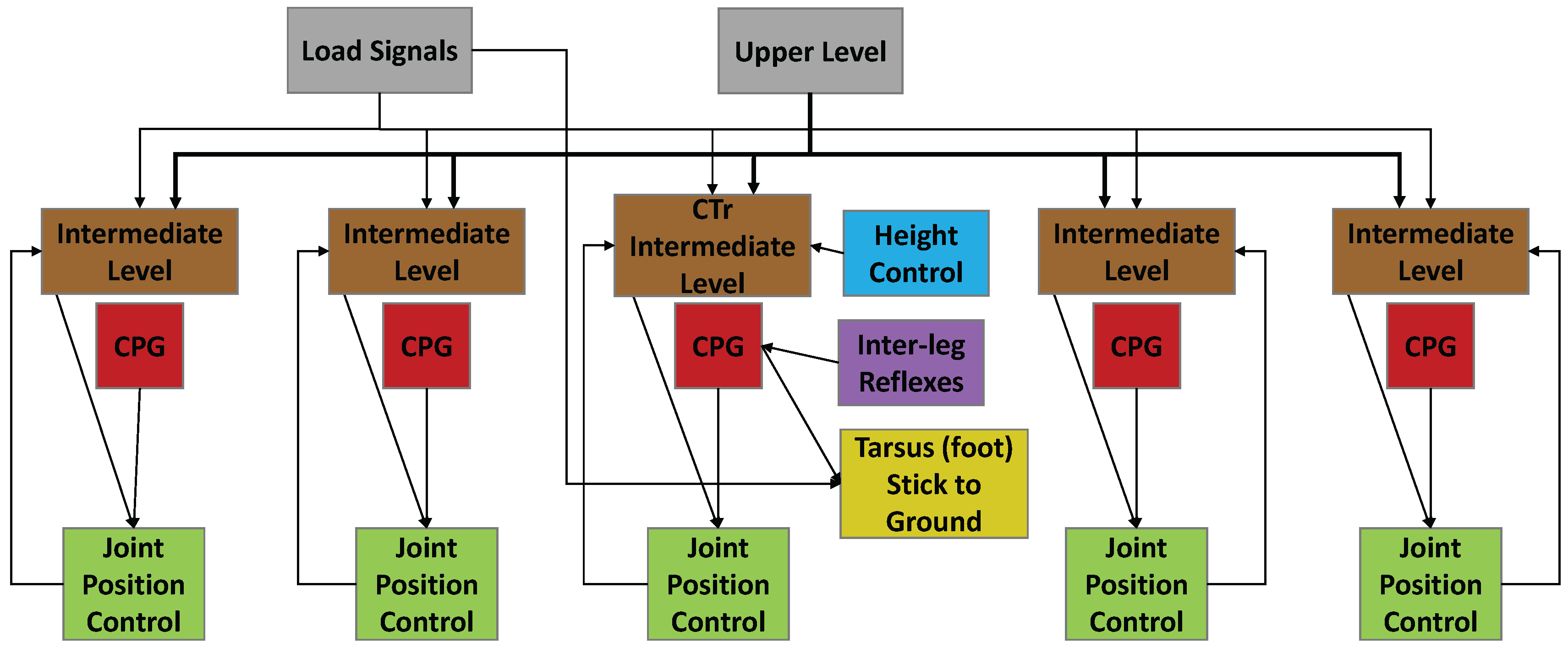
The SNS used to control SimRoach2 is a distributed network made up of functional subnetworks [26,40] (Figure 3). In short, the network functions as follows. A high-level network (gray, Figure 3) sends commands to the thoracic ganglia to stand or walk, and in which direction to walk. Each leg joint control network in each ganglion interprets this signal to decode the direction and amplitude of joint rotation in stance phase (brown, Figure 3). Each joint in the leg has a central pattern generator (CPG) that generates alternating neural activity (red, Figure 3). These have no direct neural connections between them [2]. The descending commands and CPG together establish a commanded position for each joint. Each low level joint controller (green, Figure 3) receives the commanded position signal, moves the joint to that position, and signals its position back to the intermediate (i.e., inter-joint and intra-leg) network. This intermediate network controls the transitions between stance and swing phase, by causing CTr (joints act between the coxa and the trochanter) levation when the other leg joints have reached their posterior extreme position (PEP), and causing CTr depression when the other leg joints have reached their anterior extreme position (AEP).
Additional networks are included to coordinate the walking of multiple legs. Inter-leg reflexes (purple, Figure 3) coordinate the legs for stable walking. Height control networks (blue, Figure 3) are included to control the height of the thorax by adjusting CTr depression while in stance phase. When the leg is in stance and loaded, the tarsus is “stuck” to the ground (yellow, Figure 3).
Each leg in SimRoach2 is controlled by a network like that in Figure 3. The neural implementation of joint position control and inter-leg reflexes are provided in this article. The neural implementation used for the upper level, height control, and for freezing the tarsus in stance phase are provided in the Supplementary Materials (Section: Methods Explained). The neural implementation used in the intermediate level is published in [26], and the CPG network is published in [31]. One can download the AnimatLab 2 file to see the specifics on how the sub-networks are connected to each other (Supplementary Materials File S2). Specific parameters values of the neurons and synapses are available in the Supplementary Materials (Section: Parameter Values) and in the AnimatLab 2 source file.
2.4.2. Joint Position Control
The force and length of muscles are not easy to control, and the details of how animals control them are not known, although it is known that negative feedback reflexes play a role [41]. The primary challenge is that the muscles and exoskeleton possess many elastic elements that cancel out one another’s tension. To overcome this, we designed a neural proportional-integral (PI) network to control a limb’s position (Figure 4). We believe this is justified because arthropods have disproportionately slow muscle dynamics for their size [42], which means that their muscle membranes integrate individual spikes from excitatory motor neurons, functionally behaving as integrators [43].
The perceived position (PP) neuron receives an input current proportional to the joint’s rotation (e.g., ). The commanded position (CP) neuron uses the same relationship to specify the intended rotation of the joint. The CP and PP neuron voltages are subtracted from each other to create two “error” neurons [40] (green in Figure 4). One corresponds to the CP being greater than the PP (positive error); the other corresponds to the PP being greater than the CP (negative error). Only one of these neurons will be active at a time. Each error neuron excites the appropriate muscle’s motor neuron via a synapse tuned using optimization explained in Section 2.5.6. Exciting the motor neuron increases the tension in the muscle, correcting the error in the limb’s position and functioning as proportional negative feedback. Proportional feedback alone is not enough to guarantee that the joint will reach the CP, except in very specific cases [44]. Thus, we add an integral subnetwork (described in [31]) to eliminate the steady-state error of proportional feedback alone (orange, Figure 4). The purpose of the “Zero” neuron is to subtract out the steady state activation of the integrator. Just as with the proportional feedback, there are two integral feedback pathways (integral positive and integral negative), only one of which will be active at a time.
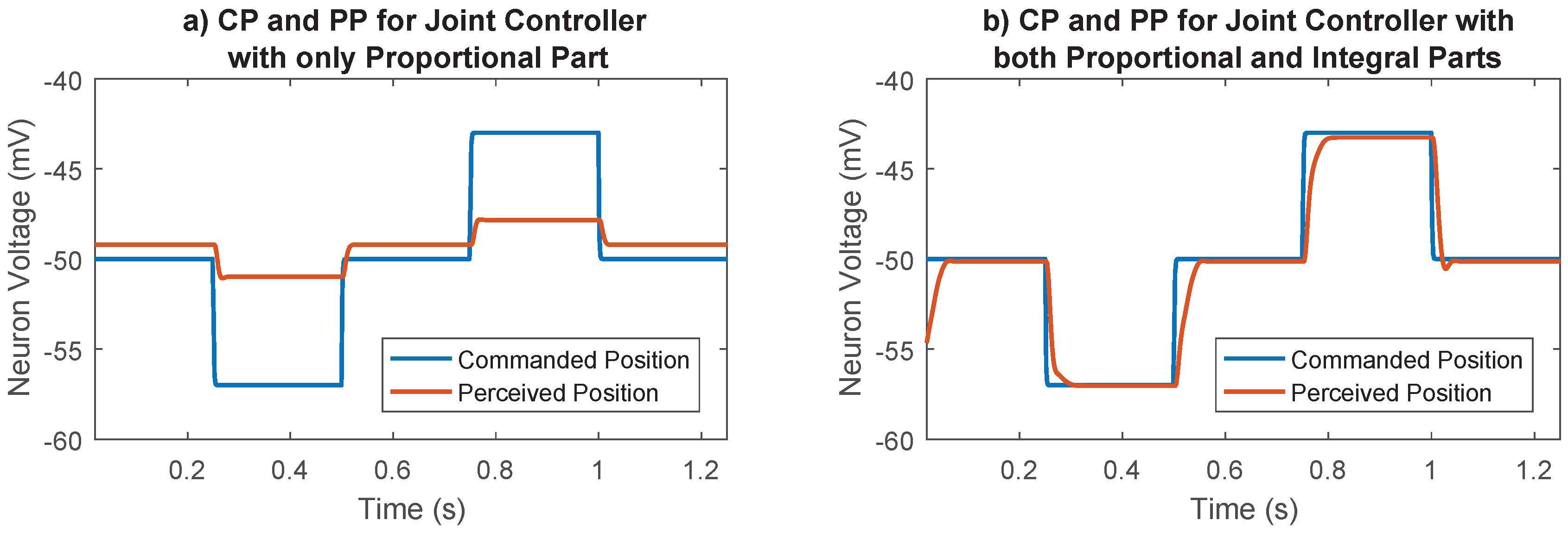
The importance of the integral part of the joint controller is shown in Figure 5. With only the proportional part, the joint does not move to its commanded position; there is always a steady state error. By adding the integral part, the steady state error is removed and the joint moves to its commanded position.
2.4.3. Inter-Leg Coordination
The legs of both insects and legged robots must communicate when they are in swing phase to ensure that the body always stays supported. Behavioral experiments have revealed correlations between the positions of different legs in arthropods [29,45], but the underlying networks remain largely unknown. Work in locusts suggests that some direct neural connections between the legs may contribute to coordination during walking [3,46]. Therefore, in SimRoach2, the levator-depressor (CTr) CPGs between legs are connected and neural pathways were engineered to produce the observed behavior.
“Holk Cruse’s rules” describe inter-leg influences that control the timing of stepping [29]. Three of these influences have been shown to be the most important to coordinate walking, and were implemented into SimRoach2. Influence 1 inhibits the start of swing phase in the rostral leg while the caudal leg is in its swing phase. Influence 2 excites the start of swing phase in the rostral leg when the caudal leg enters its stance phase. Influence 3 excites the start of swing phase in the caudal leg when the rostral leg is in stance phase, increasing in strength over time as the caudal leg is in stance phase [29]. Influences 2 and 3 are also present between contralateral legs. Table 2 summarizes these three influences. These influences are redundant, such that any perturbation to a walking gait will result in nearly immediate re-coordination of legs. The specific neural networks that were designed to replicate these three influences are shown in Figure 6. Verification of each of these networks is presented in the Supplementary Materials (Section: Methods Explained).
2.4.4. Height Control
Mechanisms to control the height of insects have been observed to exist while both walking and standing still [47,48]. However, little is known about the underlying neural mechanisms that produce these observed behaviors. Height control is important because the multiple legs form a parallel manipulator, potentially resulting in internal torques that waste energy. SimRoach2 uses a negative feedback loop to adjust CTr depression based on the length of the leg while in contact with the ground. Please see the Supplementary Materials (Section: Methods Explained) for more information.
2.5. Design Process for a Single Joint
This section describes how the parameter values of the system’s dynamical components components (e.g., muscles, joints, etc.) are selected to enable our simulated cockroach to walk. Our previous work has explained how to select parameter values for CPGs [31] and descending connectives from higher command centers that control joint motion amplitude [26]. These works, however, assumed that each joint’s control system could control the position of the joint. To apply this work to a muscle-actuated (rather than servomotor actuated) model, we first needed to select parameters for the viscoelasticity of each joint, the active and passive dynamics of each joint’s muscles, and the synaptic strengths in each joint’s controller. The name, equation number, and quantity of each are listed in Table 3.
The following sections will describe a serial design process for systematically selecting these parameter values. First, we find a rest posture for the animat. This enables us to calculate the torque on each joint due to gravity. Next, we use this gravitational torque to estimate the viscoelastic torques of the exoskeleton acting on each joint. Then, we select the muscle parameter values such that the muscles can apply enough tension to move the limb. Finally, a numerical optimization is performed to find maximum muscle activations and feedback gains that result in stable, rapid motion.
2.5.1. Resting Posture
We seek a resting posture that holds the body at a desired height above the ground, , while keeping each joint as far away from its limits as possible. This ensures that when the animat walks, it can move every joint in both directions. This process can be formulated as a constrained optimization problem. Let the vector be the configuration (i.e., joint angles) of a leg with n joints. We then define as normalized to the lower and upper bounds of motion. The i-th element of is defined as:
where and are the lower and upper bounds of joint i, respectively. This simplifies the definition of the objective function f,
where is a vector of ones. The factor of ensures that when , i.e., when every joint is in the center of its range of motion.
Let us also define as the vertical distance from the body to the foot, as computed with the forward kinematic map of the leg. We can then define the resting posture as the solution to the optimization problem:
We set , a value used for oiled plate walking experiments with cockroaches [14]. The resulting posture, shown in Figure 7, is remarkably cockroach-like. Figure 7c graphically shows the final values of on “sliders” between 0 and 1, showing that most joints are near to the center of allowed rotation. This analysis is now automated by our design toolbox KinematicOrganism [31].
2.5.2. Calculation of Passive Spring Stiffness and Damping Coefficients
The rest lengths of the passive spring and both muscles in each joint were set to the length that matched the joint angle based on the muscle attachment points. To determine the stiffness of every spring, we assumed that the animat could support its weight using the passive spring alone. This is consistent with the observation that insects’ exoskeletons are stiff even when their muscles are cut from them [35,36]. Each leg is assumed to hold an equal amount of the weight. We use the manipulator Jacobian from [49] to calculate the torques required for each joint to support its weight. Then, to calculate the stiffness of the spring, we deflect the joint a small amount (0.1 radian) and increase the stiffness of the springs until the spring produces the required torque. Detailed calculations can be found in the Supplementary Materials (Section: Methods Explained).
The damping of the passive element was calculated in the following way. For each joint, the distal joints were assumed to be held rigidly in place. This was used to compute the effective moment of inertia about the joint in question. Then, together with the stiffness value already calculated, the damping was computed to ensure that motion was overdamped, consistent with observations of insect exoskeletons [35]. Detailed calculations can be found in the Supplementary Materials (Section: Methods Explained).
2.5.3. Passive Muscle Force Parameters
After tuning the spring coefficients, the next step was to add passive muscle components. The parameters of interest for this section are muscle parameters , , and b in Equation (1). Values for these parameters vary widely from muscle-to-muscle and even from organism-to-organism [50]. Guschlbauer cited and values of approximately 6.32 N/m and 3.156 N/m (Figure 6 in [51]) while Blümel cited and values of approximately 45 N/m and 11.24 N/m (Figure 3 in [50]). Testing different values with the entire design process did not noticeably change the resulting performance of the control system, so we simply chose and values of 45 N/m and 11.24 N/m. Because the joints are already damped, we chose the small value for every muscle.
2.5.4. Active Muscle Parameters
Tuning the muscle activation parameters concerns both the muscle activation curve and the length-tension curve. Each muscle activation curve has four parameters that must be chosen: the amplitude, steepness, x-offset, and y-offset (see Equation (3)). We used data from insect muscles to pick the steepness and x-offset of the muscle activation curve such that it looked like the biologically observed data [51,52,53] (for an example, see Supplementary Materials (Section: Methods Explained)). The y-offset is constrained such that the muscle produces 0 N of active tension when the motor-neuron is at rest. The only unconstrained parameter is the maximum active tension, which is selected as part of the optimization process (see Section 2.5.6).
A muscle’ length-tension relationship reduces its ability to apply active tension as the muscle lengthens or shortens (Figure 1c). The parameter in Equation (2) defines the change in length at which the muscle can no longer contract. This parameter is chosen such that the muscle cannot apply tension at 133% and 67% of its resting length [54].
2.5.5. Synaptic Strength to Position Control Integral Neuron
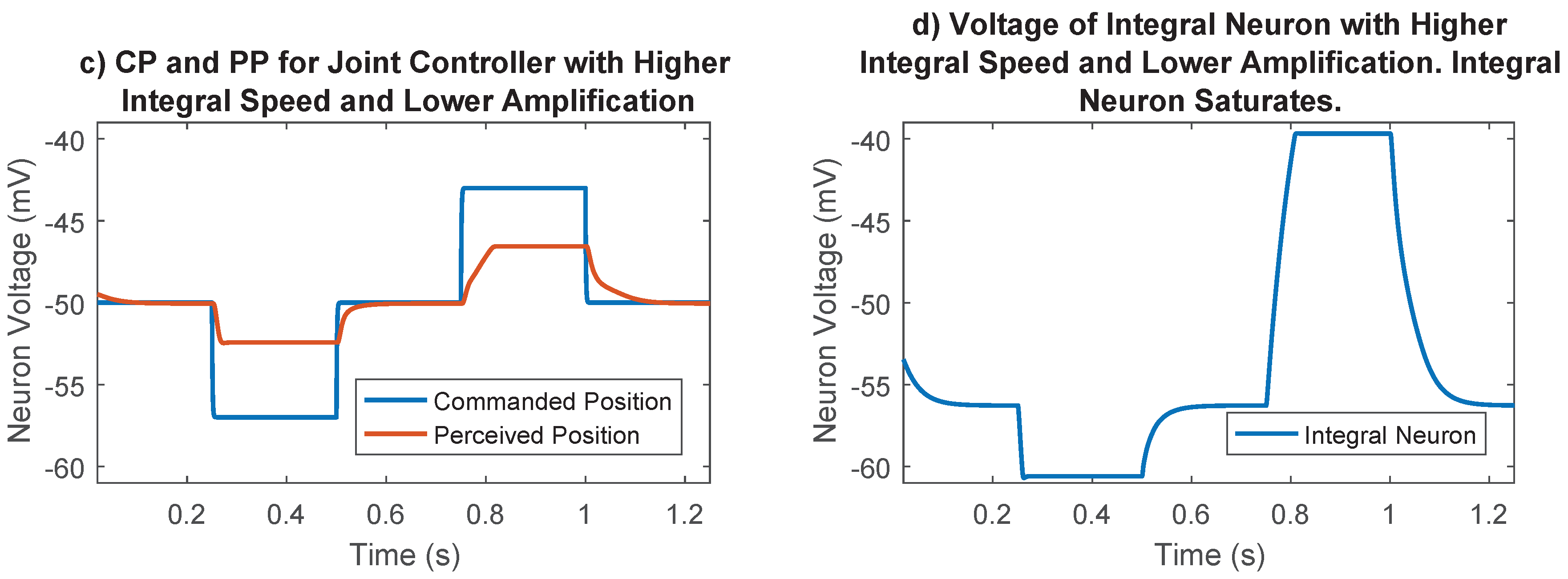
The synaptic strength between the difference neurons and the integral neuron in Figure 4 was an additional parameter that must be chosen. This parameter controls the speed of integration, and therefore the strength of the integral portion of the joint control network. The integrator could saturate if this synaptic strength was too high (for example, Figure 8), so it was set to 10 , a value that prevented saturation in most cases. The synaptic output of this network was later numerically optimized, enabling us to fine-tune the integral feedback in the controller.
2.5.6. Optimization Process
The last part of our design method is the optimization of four parameters per joint: , , , . and are the synapse strengths from the difference and integral positive and negative neurons in the joint position control network, respectively (Effectively the proportional and integral gain of the feedback controller, respectively; Figure 4). and are the amplitudes of the muscle stimulus-tension curves (Equation (3)). These parameters together determine the stiffness and torque output of each joint. The optimization was automated for each joint in our SimScan tool (Section 2.1). For each joint, an identical, four-step reference trajectory was provided, and the following objective function, , was minimized using MATLAB’s built in fmincon function, an interior-point, gradient-based nonlinear program solver:
This function calculates the squared deviation of the tracking performance from the desired values. This value is computed separately for each step in the reference trajectory, and added for all four steps to evaluate one parameter value combination. In our trials, desiredOvershoot, desiredRiseTime, and desiredSettlingTime where chosen to be 0, 0.02, and 0.03, respectively. The factors of 1000 were included to weight the different terms in approximately equally.
Every joint’s parameters were optimized to track the commanded position very well (Figure 9). One example of a joint controller’s reference tracking before and after optimization is included. This chosen case, while still good, was the worst joint in terms of reference tracking; the other 29 joints that were optimized produced even better reference tracking results.
3. Results
To show that the design method works, and that SimRoach2 will enable us to explore the control of insect locomotion, we need to show that the resulting model can indeed walk. In this section, we present data and video of SimRoach2, and compare it to data from cockroaches. All data were collected in simulation using AnimatLab 2.
3.1. Forward Walking
A video showing the walking of SimRoach2 is attached with this paper in the Supplementary Materials (Video S1). Figure 10 shows the walking path and walking speed of SimRoach2. The walking speed is calculated by smoothing and differentiating the total distance walked. After a transient startup, SimRoach2 walks in a straight path, with insect-like side-to-side motion (Figure 10). The speed of SimRoach2 in steady state is just below 20 cm/s (Figure 10).
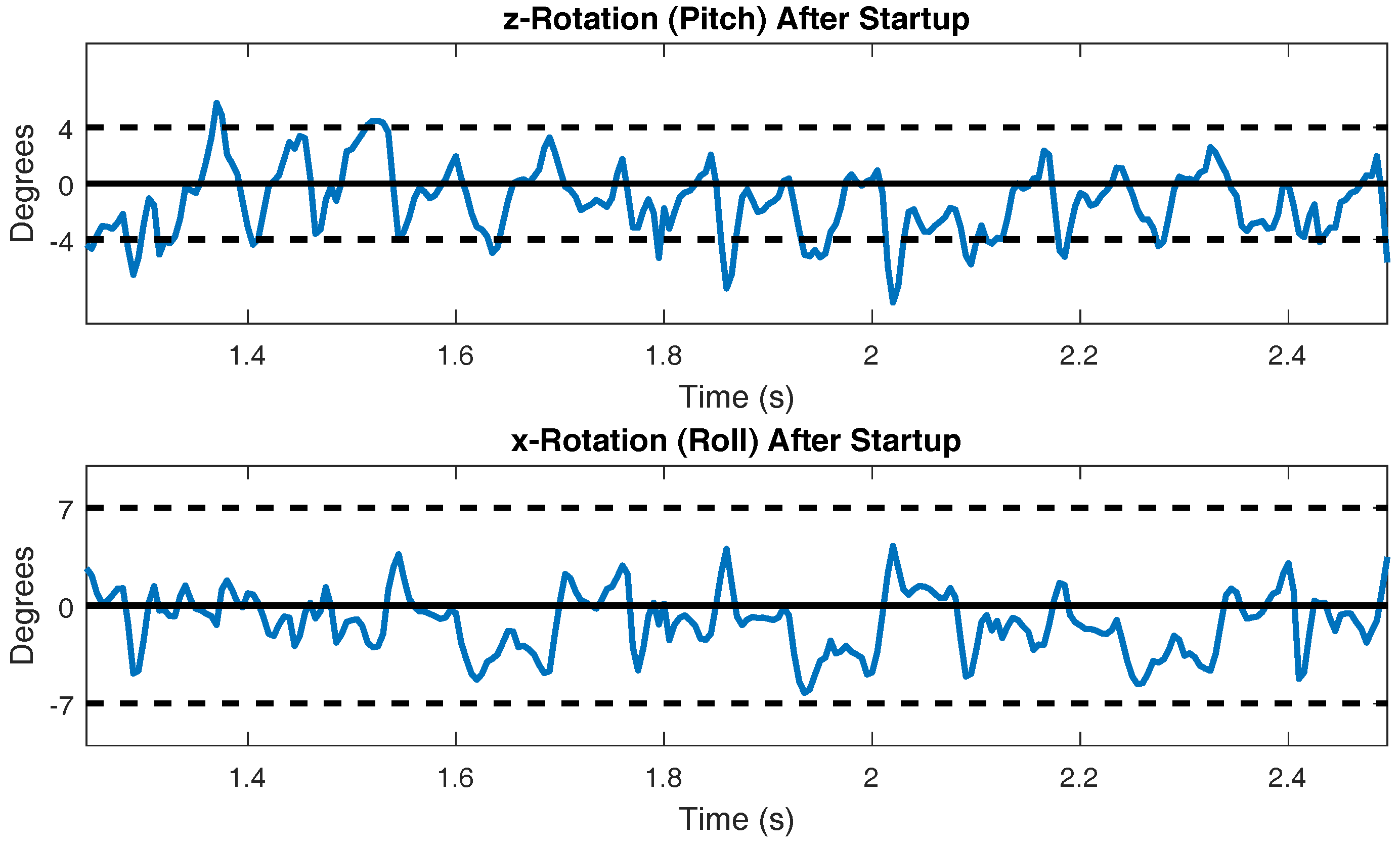
The pitch and roll of the body during steady state walking is presented in Figure 11. Actual cockroach data presented in [55] measured the pitch to be ±4 degrees and the roll to be ±7 degrees. These reference lines are plotted in Figure 11 to allow for comparison.
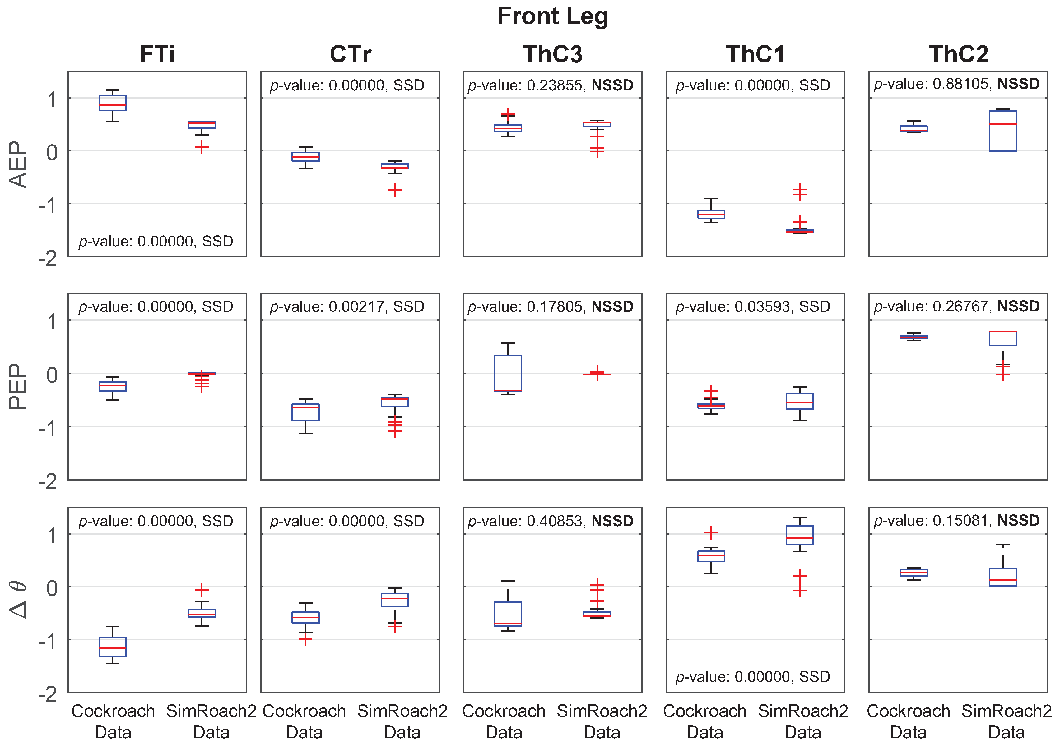
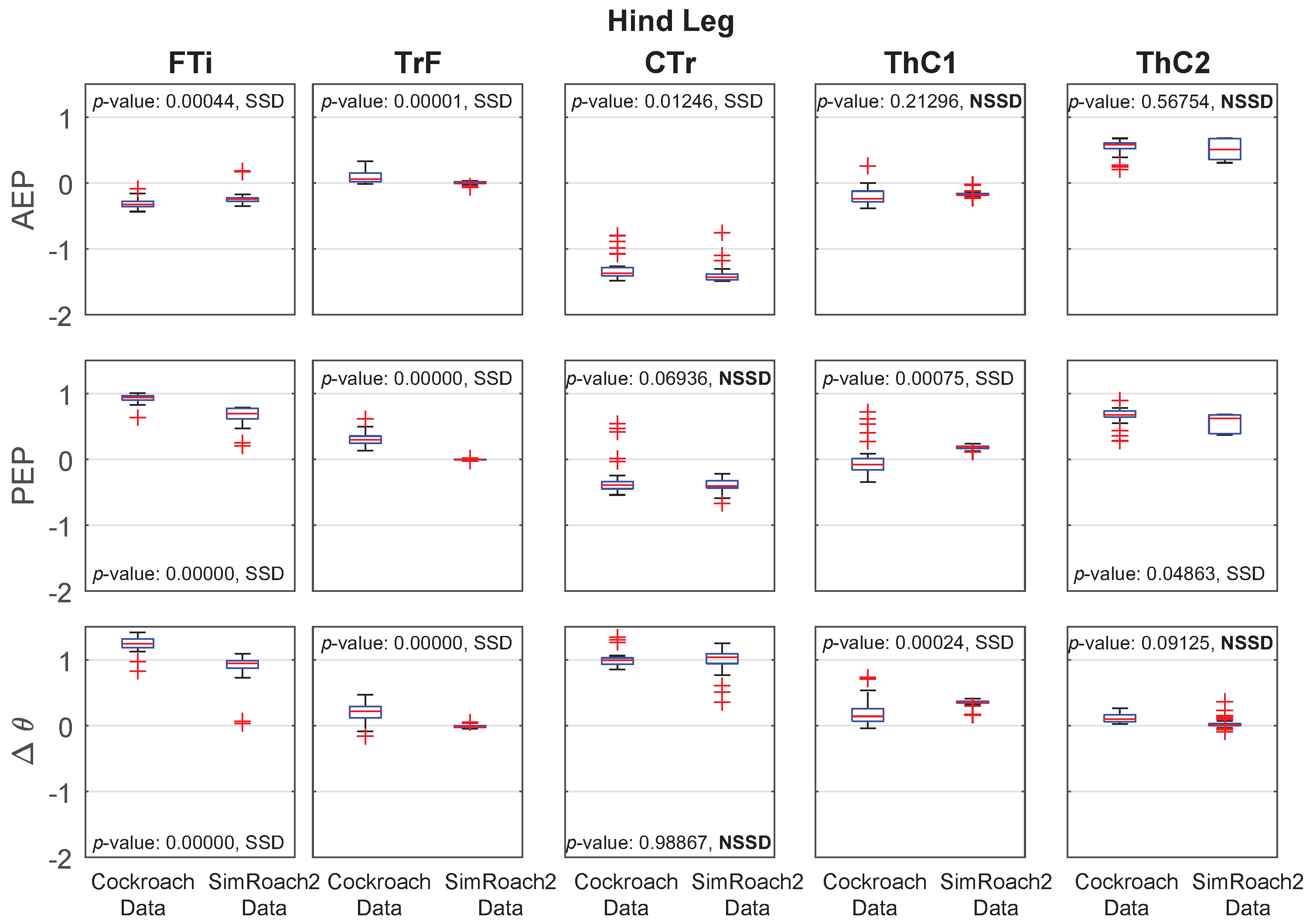
Individual joint kinematic data from both SimRoach2 and a cockroach are presented in Figure 12, Figure 13 and Figure 14. The cockroach data used for comparison was taken from [14]. For each joint in each leg during simulated walking, the joint angle at the AEP and PEP were measured for a number of steps. was calculated by subtracting the AEP from the PEP. Details on the specific method for calculated the AEP and PEP from raw data are provided in the Supplementary Materials (Section: Methods Explained).
3.2. Inter-Leg Coordination
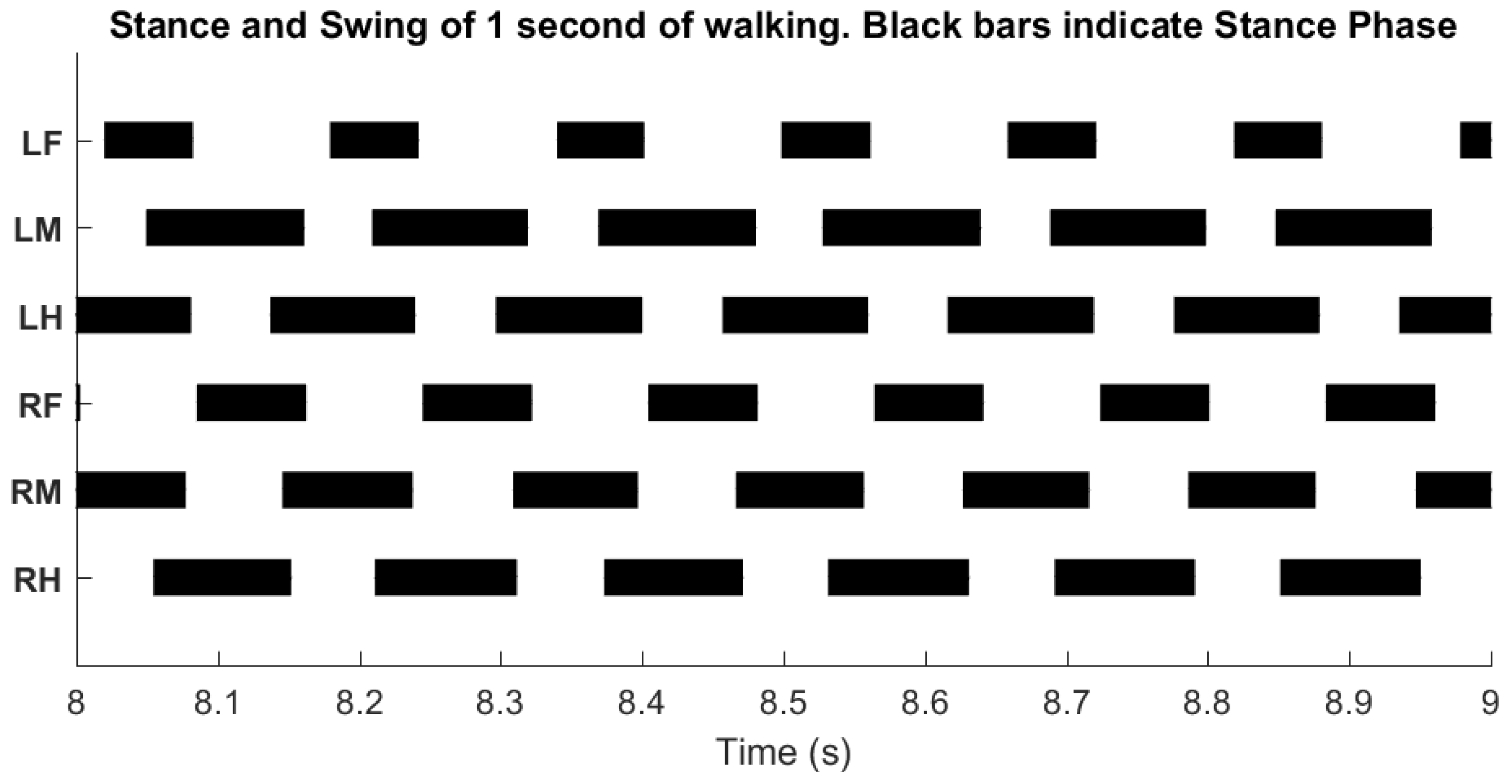
The inter-leg connections of SimRoach2 were based on biological observations and designed to enforce a tripod gait. Cockroaches walk and run almost exclusively with a tripod gait [56]. The three different inter-leg influences (Table 2) were redundant in that any perturbation to the gait would result in the near immediate re-coordination of the legs. The result of these inter-leg influences show that SimRoach2 walks with a tripod gait (Figure 15).
4. Discussion and Future Work
A cockroach model actuated by an antagonistic pair of muscles and controlled by a synthetic nervous system, informed by the current state of knowledge of insect nervous systems, successfully walked in a simulated environment. The basic parameters of locomotion are consistent with cockroaches, and this model will enable us to study more sophisticated control questions in the future. The primary challenge in this study is tuning the large number of parameter values for proper locomotion. A parameter selection process was developed that heavily depends on biological observations, and sets the few remaining parameters based on desired engineering performance.
This work improves upon the performance of a previously published neuromechanical model [57]. Since then, we have developed several methods for tuning neuron dynamics [31,40] and muscle dynamics. Most of this research has been applied to our robot MantisBot. The presented work used what has been learned in the past few years to improve upon our original simulated cockroach model such that it better reflects the biomechanics and nervous system in the animal [58]. Studying the control of more complex locomotion, such as walking in a curve or changing speed, require reliable control of the muscles actuating each joint, a functionality not incorporated in our original model. Other networks that improved the reliability of walking, such as height control and inter-leg influences, were also designed and implemented.
Many parameters required tuning for proper operation, so a design process was developed to choose these parameters based on biological data and observations, and engineering usefulness. Most of the system’s parameters are constrained by the geometry of the body, and a few are selected via numerical optimization. We believe that the presented design process is generic enough to be applied to any neuromechanical model of an insect.
In addition to enabling SimRoach2 to walk stably, two of our previously developed MATLAB design tools (KinematicOrganism [26], FeedbackDesign [31]) were improved. Before this work, all of the tools were built around working with the servomotors that MantisBot uses. Understanding the nervous system, however, requires understanding muscle dynamics, because they ultimately transform neural activity into behavior. Integrating muscle compatibility to the tools will enable us to explore how the nervous system uses muscles to produce motion. If one was interested in making their own hexapod model using our method, one could create a new hexapod model in AnimatLab 2 and tune parameters using our design tool KinematicOrganism (see Supplementary Materials File S3). To that note, KinematicOrgranism does assume a certain structure to the network, but one could potentially modify the program to tune different network structures.
4.1. Importance of Simulated Animats for Biologically-Inspired Robots
Biologists and roboticists study animal locomotion in different ways with different goals in mind. Although their goals are different, the research and findings of each side advances the other. At the intersection between biology and robots are animats such as SimRoach2. Animats facilitate the interaction between robotics and biology, enabling biologists to test hypotheses quantitatively [15,17], which leads to new understanding that can eventually be incorporated into robot designs.
While SimRoach2 can be improved in many ways, it has served as a useful model of insect locomotion. Much of the SNS used to control SimRoach2 is the same as the controller for our robot MantisBot. This work has demonstrated the potential of SNS for controlling locomotion at different scales and of differing geometry. Additionally, exploring and testing inter-leg connections on a robot’s hardware is challenging and there is a risk of breaking parts; so, testing inter-leg connections with simulated models such as SimRoach2 is useful. Lastly, much of this work involved learning about and improving muscle-actuated locomotion, and we know that muscle-like controllers are useful for robotic locomotion [59].
4.2. Walking Comparison between SimRoach2 and a Cockroach
The main goal of this work was to develop a design method for an insect model actuated with an antagonistic pair of muscles. To show that the design method works, walking data was collected and presented. In this section, the data from SimRoach2 is compared to a cockroach.
It is important to note that the cockroach kinematic data was not used during the design process. We did not design our model to “match” this data. We believe that the walking data of our model and a cockroach are similar is because of the detailed work that went into the many different parts of this model and because the model was informed by the biomechanics and nervous system of the animal. These results are a consequence of our process, and the fact that there are some similarities suggest that this model captures some of the underlying principles.
When commanded to walk forward, SimRoach2 walks straight after reaching steady state (Figure 10). The exact path of the body does include some side to side wobble, but this is also seen in cockroaches [55]. It is interesting to note that in SimRoach2, there is no correction mechanism to alter the path against error. The straight walking path is a result of the completeness of the design method in this paper. In the future, we will apply our work on directional stepping with MantisBot [60] to SimRoach2, giving us a complete-body model with which we can develop a model of the central complex, a region of the brain implicated in the control of walking speed and direction [11].
The walking speed of SimRoach2 is just below 20 cm/s (Figure 10). This is similar to cockroach data presented in [61] for free walking. The pitch and roll of a walking cockroach were measured to be between ±4 degrees and ±7 degrees, respectively [55]. SimRoach2 walks with pitch rotations just slightly outside these limits and with roll rotations well within these limits (Figure 11). Again, we believe that our results are similar to that of a cockroach because of the detailed work that went into many different parts of SimRoach2, and this similarity will serve as a launching point for future studies on locomotion.
Joint Angle Comparison
For most joints in SimRoach2, the positions of the AEP and PEP appear to match fairly well, especially compared to the range of motion of these joints (Figure 12, Figure 13 and Figure 14), suggesting that the change between stance and swing phase happens at similar positions in each leg. The means of the data sets were also compared using statistical t-tests. Of the 30 tests on the AEP and PEP for the 15 joints, 20 of the tests showed a statistically significant difference between the animal and animat. It is difficult to know if the model needs to capture these small details to inform neurobiology or robotics. Past studies of insect locomotion have focused on the changes in individual joints’ range of motion between different conditions [14,27]. As we increase the complexity of SimRoach2’s locomotion, we plan to take a similar approach; not focusing as much on how the joint kinematics match the animal, as much as how they change in different scenarios. We believe such changes help reveal what parameters the nervous system is controlling during locomotion.
4.3. Redundant Parameters
Throughout the duration of this work, it was found that many parameter values were redundant in that their overall effect on the system was very similar. For example, the angular velocity of a joint could be modulated by (1) changing the amplitude of the muscle activation curve, (2) changing the synapse strengths from the proportional or (3) integral part to the motor-neurons; or (4) changing the synapse strength to the integral neuron. Because of these parameter redundancies, it is possible that a model with very different parameter values could produce very similar locomotion. This is an interesting observation, but also not that surprising. Animal experiments [52] and modeling studies alike [62] suggest that parameter values in the nervous system vary largely, even between individuals in the same species, despite indistinguishable performance. This suggests that laboring over the decision of how to tune redundant parameters is not important, as long as the resulting motion is useful.
4.4. Velocity Control for Muscles
Insects control the velocity of their legs and joints when propelling their bodies [63,64]. Modeling studies have shown that the complete continuum of gaits can be produced simply by reducing the speed of the leg in stance phase relative to swing phase, and allowing “Holk Cruse’s rules” to coordinate the legs [15]. Therefore, to study how SimRoach2 might change walking speed, our single-joint controller must be enhanced to limit joint velocity. Currently, the joints rotate to their commanded positions very quickly, so we do not observe that “fluid” motion we like to see in walking gaits. Previous work with MantisBot has shown that limiting the velocity of the servomotors, and incorporating reflexes seen in insects, together contribute to asymmetrical stance and swing phase durations, which should lead to a continuum of gaits [65]. We have already begun such work, and find that increased biological detail in fact improves the performance of the controller (Naris, Szczecinski, and Quinn, in preparation). Models of other, slower walking insects such as stick insects may be constructed in the future to more thoroughly explore how “gait” emerges in insects.
Supplementary Materials
The following are available online at https://www.mdpi.com/2076-3417/8/1/6/s1. Video S1: SimRoach2 forward walking; File S2: Animatlab 2 source files; File S3: KinematicOrganism Toolbox; Table S4: Rest lengths of spring, flexor and extensor; Table S5: Spring stiffness and damping coefficients; Table S6: Muscle amplitude and Y-offset values; Table S7: proportional and integral synapse parameter values; Table S8: Upper level synapse parameter values; Section S9: Methods explained.
Author Contributions
S.R. led the research efforts and led the preparation of this paper. N.S. aided in the research efforts, aided in preparation of this paper and provided critical oversight. R.Q. aided in the preparation of this paper and provided critical oversight.
Conflicts of Interest
The authors declare no conflict of interest.
Abbreviations
The following abbreviations are used in this manuscript:
| AEP | Anterior extreme position |
| ANN | Artificial neural network |
| CP | Commanded position |
| CPG | Central pattern generator |
| CTr | Coxa-trochanter |
| CX | Central complex |
| DOF | Degree of freedom |
| FSM | Finite state machine |
| FTi | Femur-tibia |
| HH | Hodgkin–Huxley |
| MN | Motor-neuron |
| PEP | Posterior extreme position |
| PI | Proportional-integral |
| PP | Perceived position |
| SNS | Synthetic nervous system |
| ThC | Thorax-coxa |
| TrF | Trochanter-femur |
References
- Ryckebusch, S.; Laurent, G. Rhythmic patterns evoked in locust leg motor neurons by the muscarinic agonist pilocarpine. J. Neurophysiol. 1993, 69, 1583–1595. [Google Scholar] [PubMed]
- Büschges, A.; Schmitz, J.; Bässler, U. Rhythmic patterns in the thoracic nerve cord of the stick insect induced by pilocarpine. J. Exp. Biol. 1995, 198, 435–456. [Google Scholar]
- Ryckebusch, S.; Laurent, G. Interactions between segmental leg central pattern generators during fictive rhythms in the locust. J. Neurophysiol. 1994, 72, 2771–2785. [Google Scholar] [PubMed]
- Noah, J.A.; Quimby, L.; Frazier, S.F.; Zill, S.N. Sensing the effect of body load in legs: Responses of tibial campaniform sensilla to forces applied to the thorax in freely standing cockroaches. J. Comp. Physiol. A 2004, 190, 201–215. [Google Scholar] [CrossRef] [PubMed]
- Zill, S.; Schmitz, J.; Büschges, A. Load sensing and control of posture and locomotion. Arthropod Struct. Dev. 2004, 33, 273–286. [Google Scholar] [CrossRef] [PubMed]
- Akay, T.; Haehn, S.; Schmitz, J.; Büschges, A. Signals From Load Sensors Underlie Interjoint Coordination During Stepping Movements of the Stick Insect Leg. J. Neurophysiol. 2004, 92, 42–51. [Google Scholar] [CrossRef] [PubMed]
- Bucher, D.; Akay, T.; DiCaprio, R.a.; Buschges, A. Interjoint coordination in the stick insect leg-control system: The role of positional signaling. J. Neurophysiol. 2003, 89, 1245–1255. [Google Scholar] [CrossRef] [PubMed]
- Hess, D.; Büschges, A. Role of Proprioceptive Signals From an Insect Femur-Tibia Joint in Patterning Motoneuronal Activity of an Adjacent Leg Joint. J. Neurophysiol. 1999, 81, 1856–1865. [Google Scholar] [PubMed]
- Mu, L.; Ritzmann, R.E. Kinematics and motor activity during tethered walking and turning in the cockroach, Blaberus discoidalis. J. Comp. Physiol. A 2005, 191, 1037–1054. [Google Scholar] [CrossRef] [PubMed]
- Hellekes, K.; Blincow, E.; Hoffmann, J.; Buschges, A. Control of reflex reversal in stick insect walking: Effects of intersegmental signals, changes in direction, and optomotor-induced turning. J. Neurophysiol. 2012, 107, 239–249. [Google Scholar] [CrossRef] [PubMed]
- Martin, J.P.; Guo, P.; Mu, L.; Harley, C.M.; Ritzmann, R.E. Central-Complex Control of Movement in the Freely Walking Cockroach. Curr. Biol. 2015, 25, 2795–2803. [Google Scholar] [CrossRef] [PubMed]
- Buschmann, T.; Ewald, A.; von Twickel, A.; Büschges, A. Controlling legs for locomotion-insights from robotics and neurobiology. Bioinspir. Biomim. 2015, 10, 041001. [Google Scholar] [CrossRef] [PubMed]
- Daun-Gruhn, S. A mathematical modeling study of inter-segmental coordination during stick insect walking. J. Comput. Neurosci. 2011, 30, 255–278. [Google Scholar] [CrossRef] [PubMed]
- Szczecinski, N.S.; Brown, A.E.; Bender, J.A.; Quinn, R.D.; Ritzmann, R.E. A neuromechanical simulation of insect walking and transition to turning of the cockroach Blaberus discoidalis. Biol. Cybern. 2014, 108, 1–21. [Google Scholar] [CrossRef] [PubMed]
- Cruse, H.; Kindermann, T.; Schumm, M.; Dean, J.; Schmitz, J. Walknet - A biologically inspired network to control six-legged walking. Neural Netw. 1998, 11, 1435–1447. [Google Scholar] [CrossRef]
- Schilling, M.; Paskarbeit, J.; Hoinville, T.; Hüffmeier, A.; Schneider, A.; Schmitz, J.; Cruse, H. A hexapod walker using a heterarchical architecture for action selection. Front. Comput. Neurosci. 2013, 7, 126. [Google Scholar] [CrossRef] [PubMed]
- Ekeberg, Ö.; Blümel, M.; Büschges, A. Dynamic simulation of insect walking. Arthropod Struct. Dev. 2004, 33, 287–300. [Google Scholar] [CrossRef] [PubMed]
- Rutter, B.L.; Taylor, B.K.; Bender, J.A.; Blümel, M.; Lewinger, W.A.; Ritzmann, R.E.; Quinn, R.D. Descending commands to an insect leg controller network cause smooth behavioral transitions. In Proceedings of the IEEE International Conference on Intelligent Robots and Systems, San Francisco, CA, USA, 25–30 September 2011; pp. 215–220. [Google Scholar]
- Daun-Gruhn, S.; Tóth, T.I. An inter-segmental network model and its use in elucidating gait-switches in the stick insect. J. Comput. Neurosci. 2011, 31, 43–60. [Google Scholar] [CrossRef] [PubMed]
- Toth, T.I.; Schmidt, J.; Büschges, A.; Daun-Gruhn, S. A Neuro-Mechanical Model of a Single Leg Joint Highlighting the Basic Physiological Role of Fast and Slow Muscle Fibres of an Insect Muscle System. PLoS ONE 2013, 8, e78247. [Google Scholar] [CrossRef] [PubMed]
- Tóth, T.I.; Grabowska, M.; Rosjat, N.; Hellekes, K.; Borgmann, A.; Daun-Gruhn, S. Investigating inter-segmental connections between thoracic ganglia in the stick insect by means of experimental and simulated phase response curves. Biol. Cybern. 2015, 109, 349–362. [Google Scholar] [CrossRef] [PubMed]
- Schilling, M.; Hoinville, T.; Schmitz, J.; Cruse, H. Walknet, a bio-inspired controller for hexapod walking. Biol. Cybern. 2013, 107, 397–419. [Google Scholar] [CrossRef] [PubMed]
- Schmitz, J.; Schneider, A.; Schilling, M.; Cruse, H. No need for a body model: Positive velocity feedback for the control of an 18-DOF robot walker. Appl. Bionics Biomech. 2008, 5, 135–147. [Google Scholar] [CrossRef]
- Dupeyroux, J.; Passault, G.; Ruffier, F.; Viollet, S.; Serres, J. Hexabot: A small 3D-printed six-legged walking robot designed for desert ant-like navigation tasks. In Proceedings of the IFAC Word Congress, Toulouse, France, 9–14 July 2017. [Google Scholar]
- Szczecinski, N.S.; Getsy, A.P.; Martin, J.P.; Ritzmann, R.E.; Quinn, R.D. Mantisbot is a robotic model of visually guided motion in the praying mantis. Arthropod Struct. Dev. 2017, 46, 736–751. [Google Scholar] [CrossRef] [PubMed]
- Szczecinski, N.S.; Quinn, R.D. Template for the neural control of directed stepping generalized to all legs of MantisBot. Bioinspir. Biomim. 2017, 12, 045001. [Google Scholar] [CrossRef] [PubMed]
- Gruhn, M.; Hoffmann, O.; Dübbert, M.; Scharstein, H.; Büschges, A. Tethered stick insect walking: A modified slippery surface setup with optomotor stimulation and electrical monitoring of tarsal contact. J. Neurosci. Methods 2006, 158, 195–206. [Google Scholar] [CrossRef] [PubMed]
- Durr, V. The behavioural transition from straight to curve walking: Kinetics of leg movement parameters and the initiation of turning. J. Exp. Biol. 2005, 208, 2237–2252. [Google Scholar] [CrossRef] [PubMed]
- Cruse, H. What mechanisms coordinate leg movement in walking arthropods? Trends Neurosci. 1990, 13, 15–21. [Google Scholar] [CrossRef]
- Cofer, D.; Cymbalyuk, G.; Reid, J.; Zhu, Y.; Heitler, W.J.; Edwards, D.H. AnimatLab: A 3D graphics environment for neuromechanical simulations. J. Neurosci. Methods 2010, 187, 280–288. [Google Scholar] [CrossRef] [PubMed]
- Szczecinski, N.S.; Hunt, A.J.; Quinn, R.D. Design process and tools for dynamic neuromechanical models and robot controllers. Biol. Cybern. 2017, 111, 105–127. [Google Scholar] [CrossRef] [PubMed]
- Hodgkin, A.L.; Huxley, A.F. A quantitative description of membrane current and its application to conduction and excitation in nerve. Bull. Math. Biol. 1990, 52, 25–71. [Google Scholar] [CrossRef] [PubMed]
- Hill, A.V. The Heat of Shortening and the Dynamic Constants of Muscle. Proc. R. Soc. B Biol. Sci. 1938, 126, 136–195. [Google Scholar] [CrossRef]
- Shadmehr, R.; Arbib, M.A. A mathematical analysis of the force-stiffness characteristics of muscles in control of a single joint system. Biol. Cybern. 1992, 66, 463–477. [Google Scholar] [CrossRef] [PubMed]
- Hooper, S.L.; Guschlbauer, C.; Blumel, M.; Rosenbaum, P.; Gruhn, M.; Akay, T.; Buschges, A. Neural Control of Unloaded Leg Posture and of Leg Swing in Stick Insect, Cockroach, and Mouse Differs from That in Larger Animals. J. Neurosci. 2009, 29, 4109–4119. [Google Scholar] [CrossRef] [PubMed]
- Ache, J.M.; Matheson, T. Passive Joint Forces Are Tuned to Limb Use in Insects and Drive Movements without Motor Activity. Curr. Biol. 2013, 23, 1418–1426. [Google Scholar] [CrossRef] [PubMed]
- Zill, S.N.; Chaudhry, S.; Exter, A.; Büschges, A.; Schmitz, J. Positive force feedback in development of substrate grip in the stick insect tarsus. Arthropod Struct. Dev. 2014, 43, 441–455. [Google Scholar] [CrossRef] [PubMed]
- Paskarbeit, J.; Otto, M.; Schilling, M.; Schneider, A. Stick(y) Insects—Evaluation of Static Stability for Bio-inspired Leg Coordination in Robotics. In Proceedings of the Conference on Biomimetic and Biohybrid Systems, Edinburgh, UK, 19–22 July 2016; Volume 1, pp. 239–250. [Google Scholar]
- Ramdya, P.; Thandiackal, R.; Cherney, R.; Asselborn, T.; Benton, R.; Ijspeert, A.J.; Floreano, D. Climbing favours the tripod gait over alternative faster insect gaits. Nat. Commun. 2017, 8, 14494. [Google Scholar] [CrossRef] [PubMed]
- Szczecinski, N.S.; Hunt, A.J.; Quinn, R.D. A functional subnetwork approach to designing synthetic nervous systems that control legged robot locomotion. Front. Neurorobot. 2017, 11, 1–19. [Google Scholar] [CrossRef] [PubMed]
- Bässler, D.; Büschges, A.; Meditz, S.; Bässler, U. Correlation between muscle structure and filter characteristics of the muscle-joint system in three orthopteran insect species. J. Exp. Biol. 1996, 199, 2169–2183. [Google Scholar]
- Wolf, H. Inhibitory motoneurons in arthropod motor control: Organisation, function, evolution. J. Comp. Physiol. A 2014, 200, 693–710. [Google Scholar] [CrossRef] [PubMed]
- Hooper, S.L.; Guschlbauer, C.; von Uckermann, G.; Buschges, A. Different Motor Neuron Spike Patterns Produce Contractions With Very Similar Rises in Graded Slow Muscles. J. Neurophysiol. 2007, 97, 1428–1444. [Google Scholar] [CrossRef] [PubMed]
- Garcia-Sanz, M. Chapter 3 P.I.D. control: Structure. In EECS 475 Applied Control; Case Western Reserve University: Cleveland, OH, USA, 2016. [Google Scholar]
- Dürr, V.; Schmitz, J.; Cruse, H. Behaviour-based modelling of hexapod locomotion: Linking biology and technical application. Arthropod Struct. Dev. 2004, 33, 237–250. [Google Scholar] [CrossRef] [PubMed]
- Mantziaris, C.; Bockemühl, T.; Holmes, P.; Borgmann, A.; Daun, S.; Büschges, A. Intra- and intersegmental influences among central pattern generating networks in the walking system of the stick insect. J. Neurophysiol. 2017, 118, 2296–2310. [Google Scholar] [CrossRef] [PubMed]
- Cruse, H.; Riemenschneider, D.; Stammer, W. Control of body position of a stick insect standing on uneven surfaces. Biol. Cybern. 1989, 61, 71–77. [Google Scholar] [CrossRef]
- Cruse, H.; Schmitz, J.; Braun, U.; Schweins, A. Control of body height in a stick insect walking on a treadwheel. J. Exp. Biol. 1993, 181, 141–155. [Google Scholar]
- Murray, R.M.; Li, Z.; Sastry, S.S. A Mathematical Introduction to Robotic Manipulation; CRC Press: Boca Raton, FL, USA, 1994. [Google Scholar]
- Blumel, M.; Hooper, S.L.; Guschlbauer, C.; White, W.E.; Buschges, A. Determining all parameters necessary to build Hill-type muscle models from experiments on single muscles. Biol. Cybern. 2012, 106, 543–558. [Google Scholar] [CrossRef] [PubMed]
- Guschlbauer, C.; Scharstein, H.; Büschges, A. The extensor tibiae muscle of the stick insect: Biomechanical properties of an insect walking leg muscle. J. Exp. Biol. 2007, 210, 1092–1108. [Google Scholar] [CrossRef] [PubMed]
- Blümel, M.; Guschlbauer, C.; Daun-Gruhn, S.; Hooper, S.L.; Büschges, A. Hill-type muscle model parameters determined from experiments on single muscles show large animal-to-animal variation. Biol. Cybern. 2012, 106, 559–571. [Google Scholar] [CrossRef] [PubMed]
- Hooper, S.L.; Guschlbauer, C.; Blümel, M.; von Twickel, A.; Hobbs, K.H.; Thuma, J.B.; Büschges, A. Muscles: Non-Linear Transformers of Motor Neuron Activity; Springer Series in Computational Neuroscience; Springer: New York, NY, USA, 2016; pp. 163–194. [Google Scholar]
- Rassier, D.; MacIntosh, B.; Herzog, W. Length dependence of active force production in skeletal muscle. J. Appl. Physiol. 1999, 86, 1445–1457. [Google Scholar] [PubMed]
- Schroer, R.; Boggess, M.; Bachmann, R.; Quinn, R.; Ritzmann, R. Comparing cockroach and Whegs robot body motions. In Proceedings of the IEEE International Conference on Robotics and Automation, New Orleans, LA, USA, 26 April–1 May 2004; Volume 4, pp. 3288–3293. [Google Scholar]
- Hughes, G.M. The Co-ordination of Insect Movements. J. Exp. Biol. 1952, 29, 267–285. [Google Scholar]
- Szczecinski, N.S. Massively Distributed Neuromorphic Control for Legged Robots Modeled after Insect Stepping. Master’s Thesis, Case Western Reserve University, Cleveland, OH, USA, 2013. [Google Scholar]
- Rubeo, S.E. Control of Simulated Cockroach Using Synthethic Nervous Systems. Master’s Thesis, Case Western Reserve University, Cleveland, OH, USA, 2017. [Google Scholar]
- Rutter, B.L.; Lewinger, W.A.; Blumel, M.; Buschges, A.; Quinn, R.D. Simple Muscle Models Regularize Motion in a Robotic Leg with Neurally-Based Step Generation. In Proceedings of the 2007 IEEE International Conference on Robotics and Automation, Roma, Italy, 10–14 April 2007; pp. 630–635. [Google Scholar]
- Szczecinski, N.S.; Getsy, A.P.; Bosse, J.W.; Martin, J.P.; Ritzmann, R.E.; Quinn, R.D. MantisBot Uses Minimal Descending Commands to Pursue Prey as Observed in Tenodera Sinensis. In Biomimetic and Biohybrid Systems; Springer International Publishing: Cham, Switzerland, 2016; pp. 329–340. [Google Scholar]
- Bender, J.A.; Simpson, E.M.; Tietz, B.R.; Daltorio, K.A.; Quinn, R.D.; Ritzmann, R.E. Kinematic and behavioral evidence for a distinction between trotting and ambling gaits in the cockroach Blaberus discoidalis. J. Exp. Biol. 2011, 214, 2057–2064. [Google Scholar] [CrossRef] [PubMed]
- Golowasch, J.; Goldman, M.S.; Abbott, L.F.; Marder, E. Failure of Averaging in the Construction of a Conductance-Based Neuron Model. J. Neurophysiol. 2002, 87, 1129–1131. [Google Scholar] [CrossRef] [PubMed]
- Cruse, H. Which Parameters Control the Leg Movement of a Walking Insect? I. Velocity Control during the Stance Phase. J. Exp. Biol. 1985, 116, 343–355. [Google Scholar]
- Gruhn, M.; von Uckermann, G.; Westmark, S.; Wosnitza, A.; Buschges, A.; Borgmann, A. Control of Stepping Velocity in the Stick Insect Carausius morosus. J. Neurophysiol. 2009, 102, 1180–1192. [Google Scholar] [CrossRef] [PubMed]
- Szczecinski, N.S.; Quinn, R.D. MantisBot Changes Stepping Speed by Entraining CPGs to Positive Velocity Feedback. In Biomimetic and Biohybrid Systems; Springer: Cham, Switzerland, 2017; pp. 440–452. [Google Scholar]
Figure 1.
Hill Muscle Model used in AnimatLab 2 (adapted from [34]). (a) The model contains a series spring, a parallel spring, a parallel damper, and an active component; (b) the length-tension curve adjusts the active tension based on the length of the muscle; (c) the stimulus-tension curve adjusts the active tension based on the voltage of the motor-neuron.
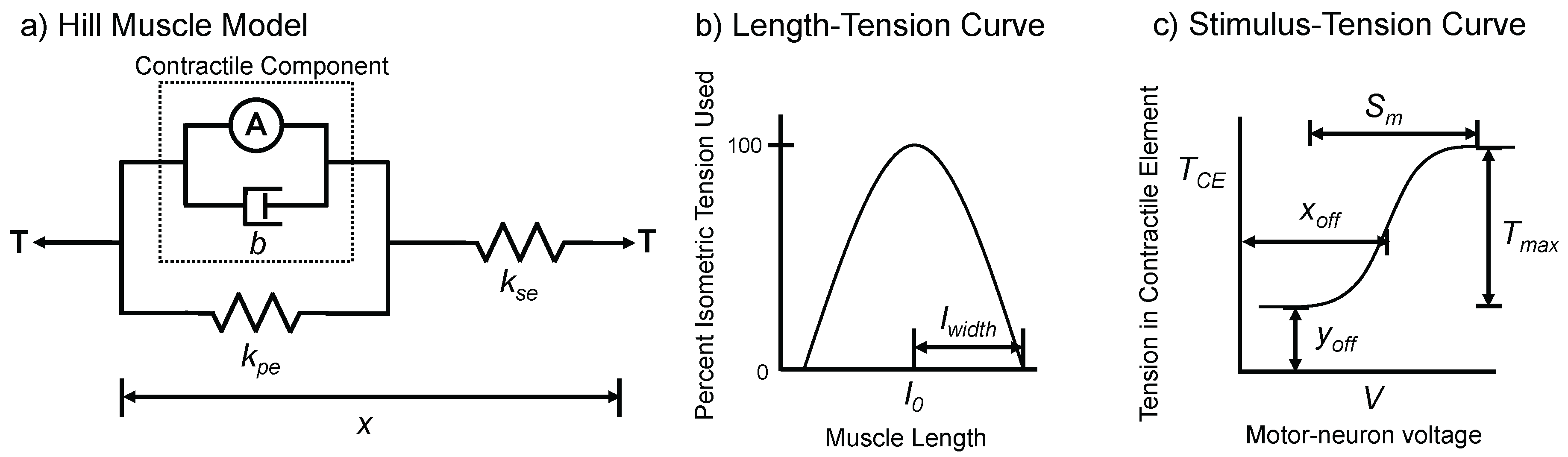
Figure 2.
Physical model of the cockroach Blaberus discoidalis. (a) Picture of SimRoach2 in AnimatLab2; (b) each joint consists of a flexor muscle, extensor muscle and a passive spring and damper attached at the same points as the flexor muscle; (c) each tarsus (foot) is attached to the tibia with a free ball and socket joint that “sticks” when in contact with the ground.
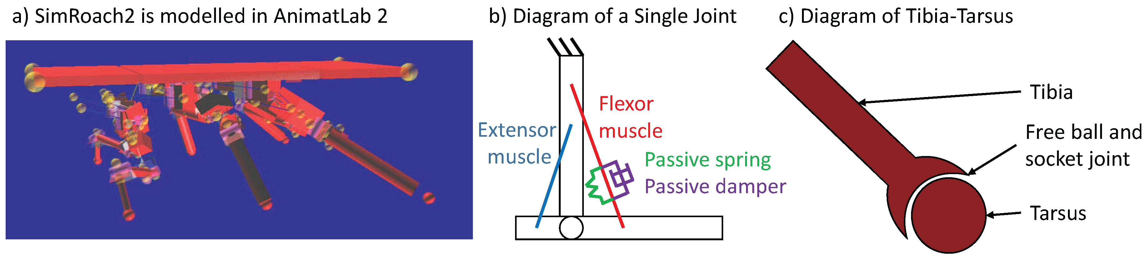
Figure 3.
Functional diagram of the synthetic nervous system used for one leg. Each leg consists of five joints. Descending commands from the higher level brain and load signals (gray) affect the intermediate network (brown). Central pattern generators (CPGs, red) generate the rhythmic movement and are present in each joint. The intermediate network and the CPGs establish a commanded position for each joint. Joint controllers (green) take the commanded position and move the joint to that position. Signals from other legs coordinate walking via inter-leg reflexes (purple). Height control networks (blue) are present in each leg. When the leg is loaded and in stance phase, the foot is frozen to the ground (yellow). Note that this is a simple functional diagram; each functional unit consists of dynamics neurons connected to each other via synapses.

Figure 4.
Diagram of the joint control network. Joint angles are linearly mapped to neuron voltage. The commanded position (CP) neuron input signal comes from the intermediate network. The perceived position (PP) neuron input signal is mapped from the length of the extensor. The CP and PP neuron voltage’s are subtracted from each other to create two “error” neurons (green). Only one of these neurons can be active at a time. The error neurons excite the appropriate muscle motor-neuron, acting in a very similar way to the proportional part of a standard PID controller. The error neurons are also used as an input to the integral part (orange). The integral part continues to adjust the appropriate motor-neuron (MN) until the voltage of the CP and PP neurons match. Synapses with black circles and white triangles represent inhibitory synapses and excitatory synapses, respectively.
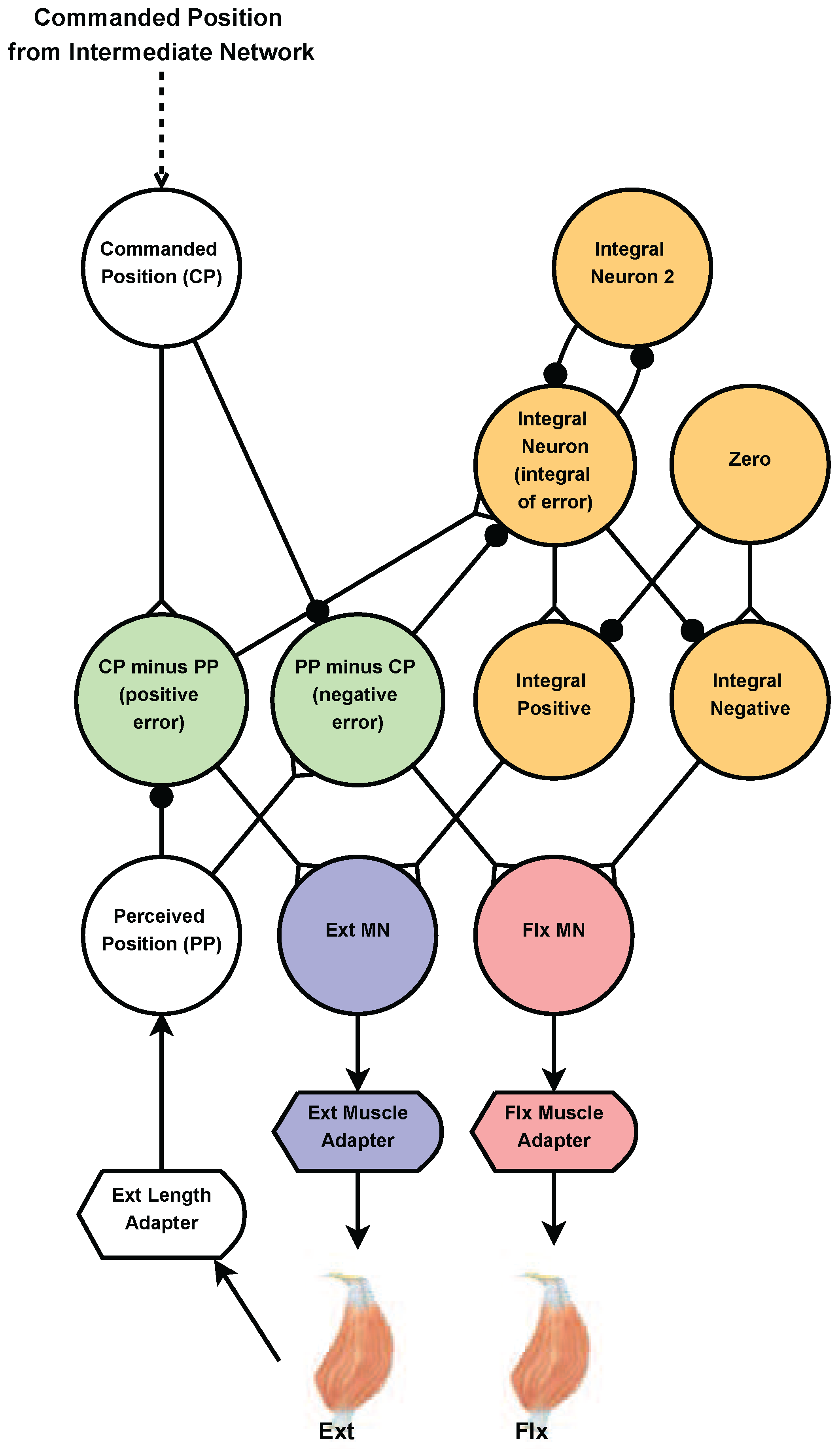
Figure 5.
Importance of the integral part in the joint control network. (a) Joint controller with integral part disabled. The proportional part alone is not enough to move the joint to the desired position. There is always a steady state error. (b) Joint controller with both proportional and integral parts. The integral part removes the steady state error.

Figure 6.
Neural Implementation of three “Holk Cruse’s rules” [29]. (a) Influence 1 inhibits the start of swing phase when the posterior leg is in its swing phase; (b) Influence 2 momentarily excites the start of swing phase in the rostral leg when the caudal leg enters its stance phase. To capture this, we use a differentiator network [40]; (c) Excites the start of swing phase while the anterior leg is in its stance phase, increasing in strength over time. To capture this, we use an integrator network [40]. Synapses with black circles and white triangles represent inhibitory synapses and excitatory synapses, respectively.
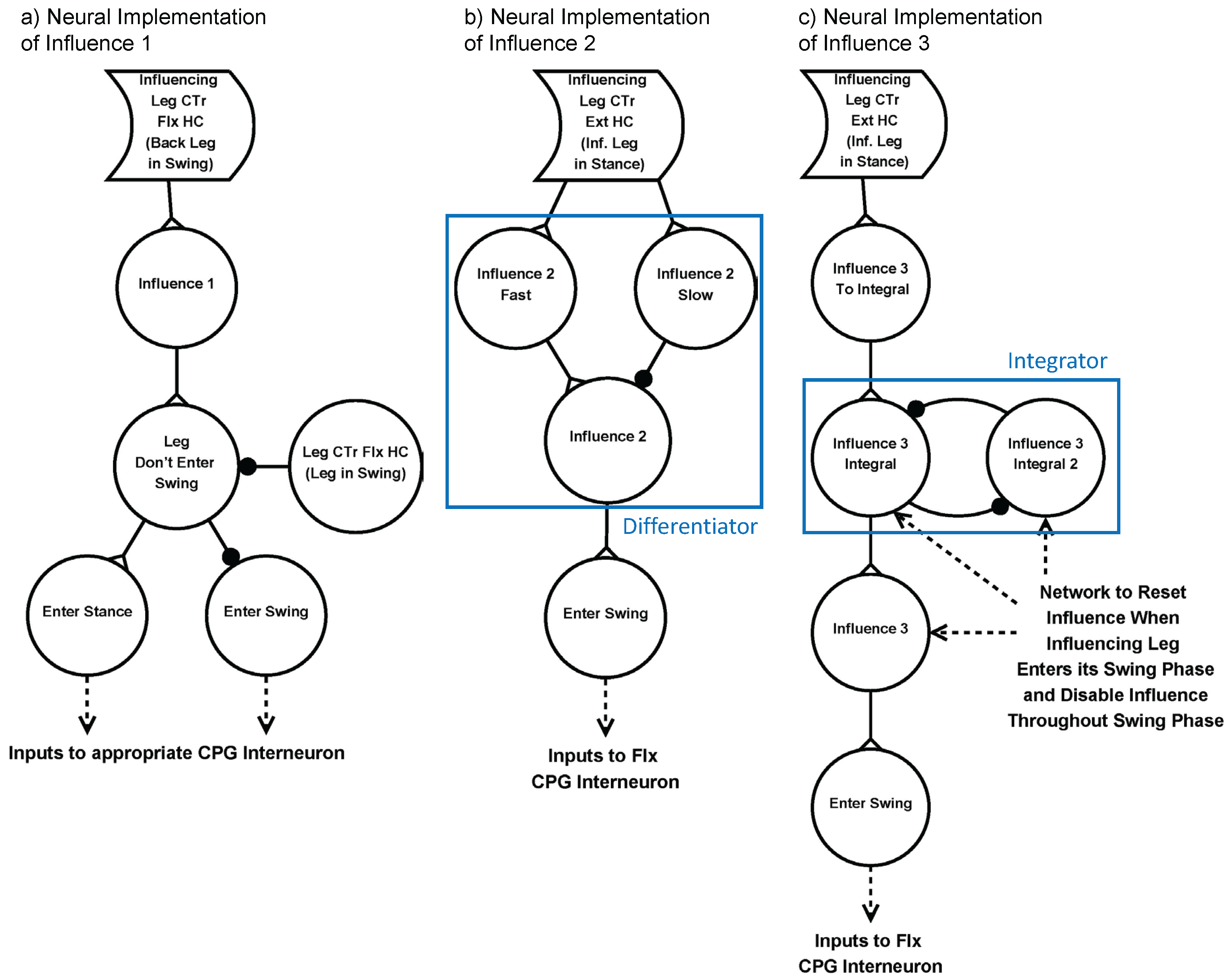
Figure 7.
Resting posture of SimRoach2. (a) Screenshot of SimRoach2 standing in AnimatLab 2; (b) rest posture of SimRoach2 calculated in MATLAB; (c) graphical representation of , the rest posture angle of each joint relative to its joint limits. No joint’s rest posture angle is near its joint limits.
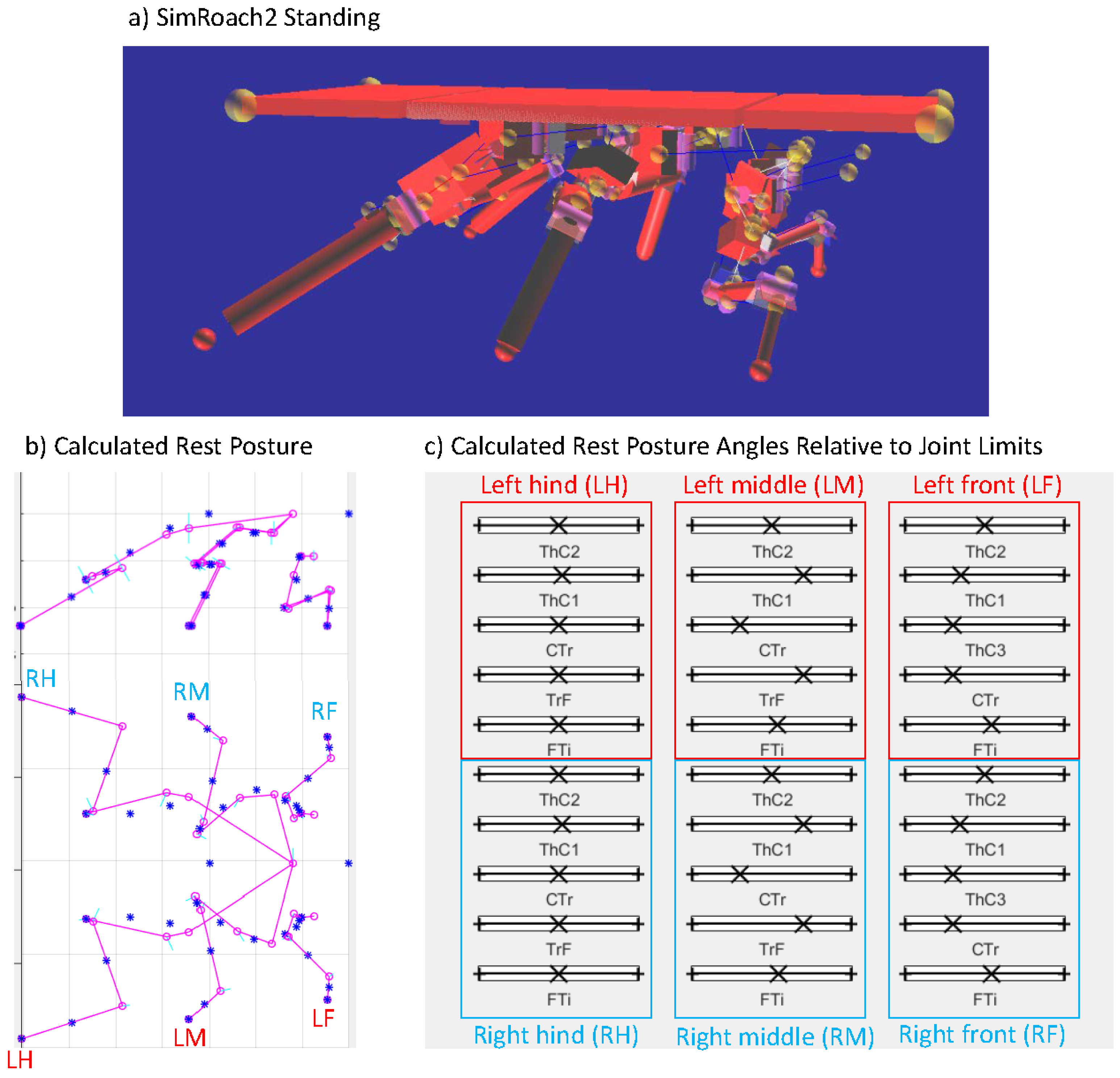
Figure 8.
Importance of synaptic strength to the integral neuron in joint position control. (a) Commanded position and perceived position for the selected case. Lower integration speed and larger amplification tuned during the optimization process results in good reference tracking; (b) Voltage of integral neuron for the selected case. Lower integral speed results in voltages far away from saturation points; (c) Commanded position and perceived position for the undesirable case. The joint never gets to its commanded position because the integral neuron saturates; (d) Voltage of integral neuron for the undesirable case. Higher integration speeds cause the integral neuron to reach the synaptic thresholds, losing its ability to send information.
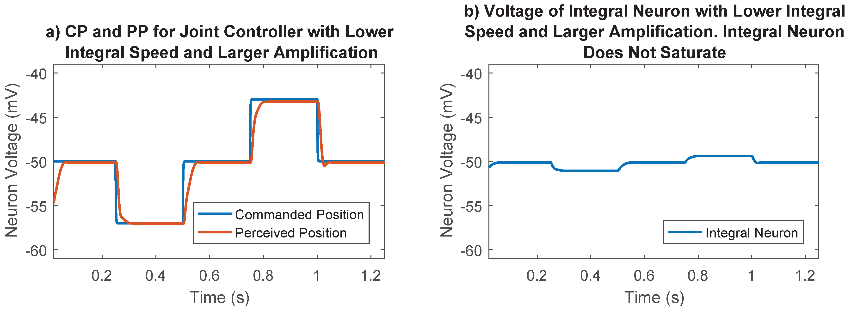

Figure 9.
Optimizing parameters , , , and improves reference tracking. The commanded position trajectory is chosen arbitrarily.
Figure 9.
Optimizing parameters , , , and improves reference tracking. The commanded position trajectory is chosen arbitrarily.
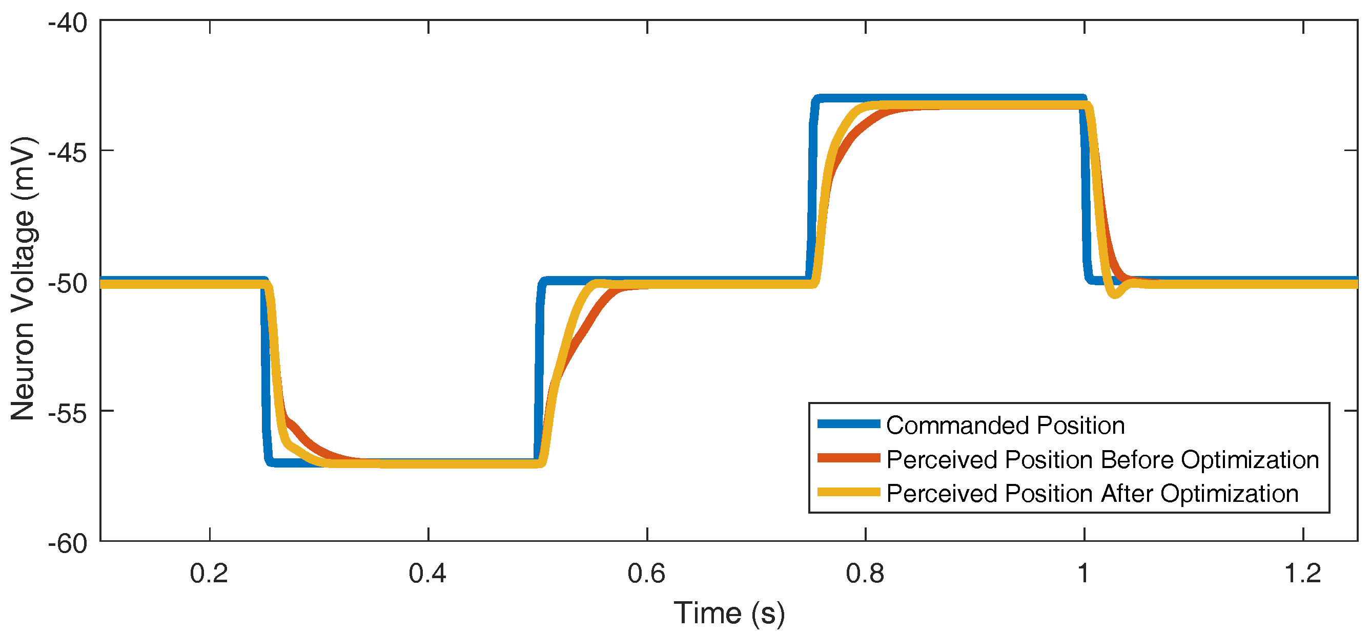
Figure 10.
Forward walking path and speed.
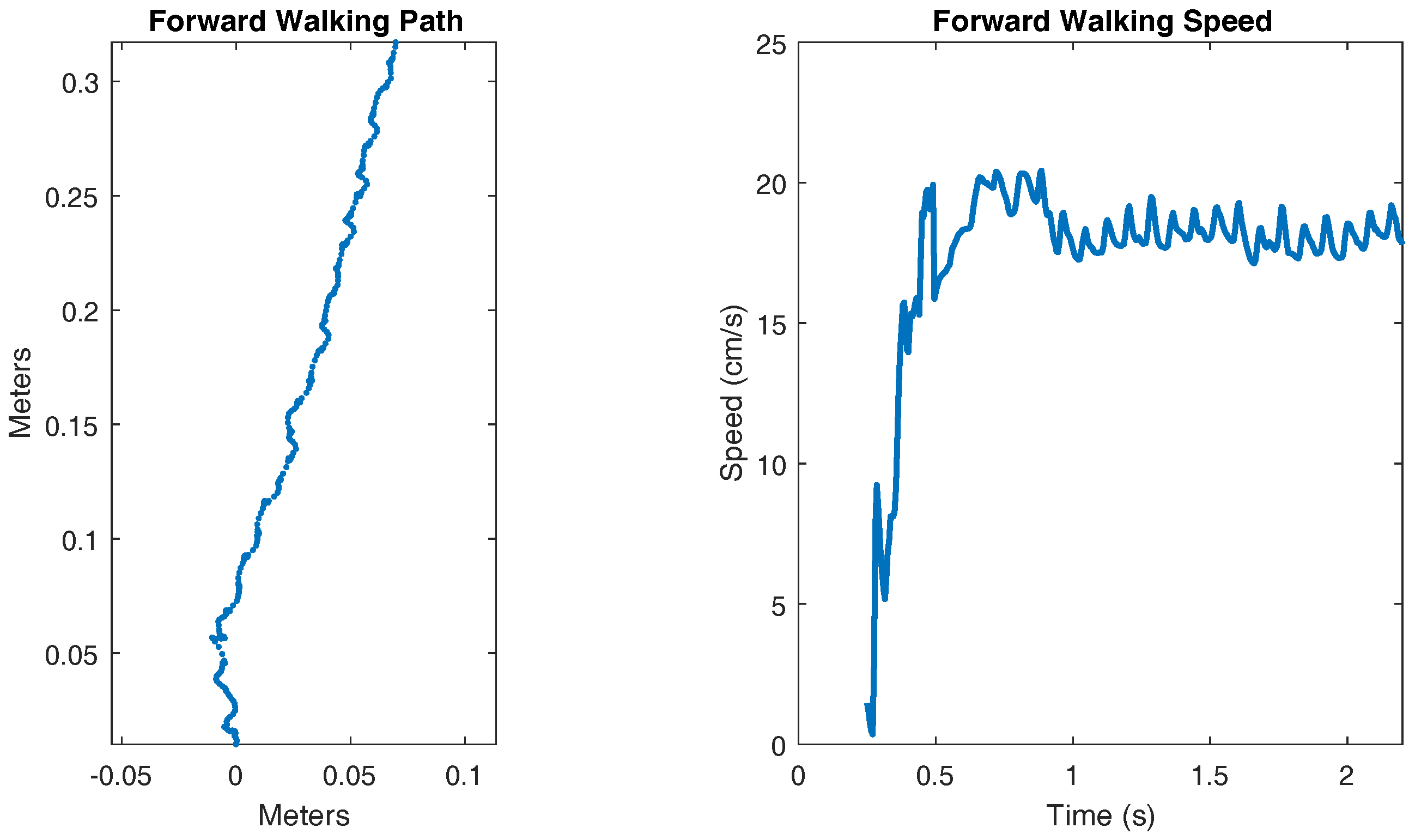
Figure 11.
Pitch and roll of the body during steady state walking.

Figure 12.
Front leg anterior extreme position (AEP), posterior extreme position (PEP), and joint angle data in a cockroach and in SimRoach2. Thirty six cockroach data points were used. Thirty three SimRoach2 data points were used. p-values from the two-sample t-tests and whether there is a statistically-significant difference (SSD, bad match) or no statistically-significant difference (NSSD, good match) between the samples are provided.

Figure 13.
Middle leg anterior extreme position (AEP), posterior extreme position (PEP), and joint angle data in a cockroach and in SimRoach2. Thirty one cockroach data points were used. Forty six SimRoach2 data points were used. p-values from the two-sample t-tests and whether there is a statistically-significant difference (SSD, bad match) or no statistically-significant difference (NSSD, good match) between the samples are provided.
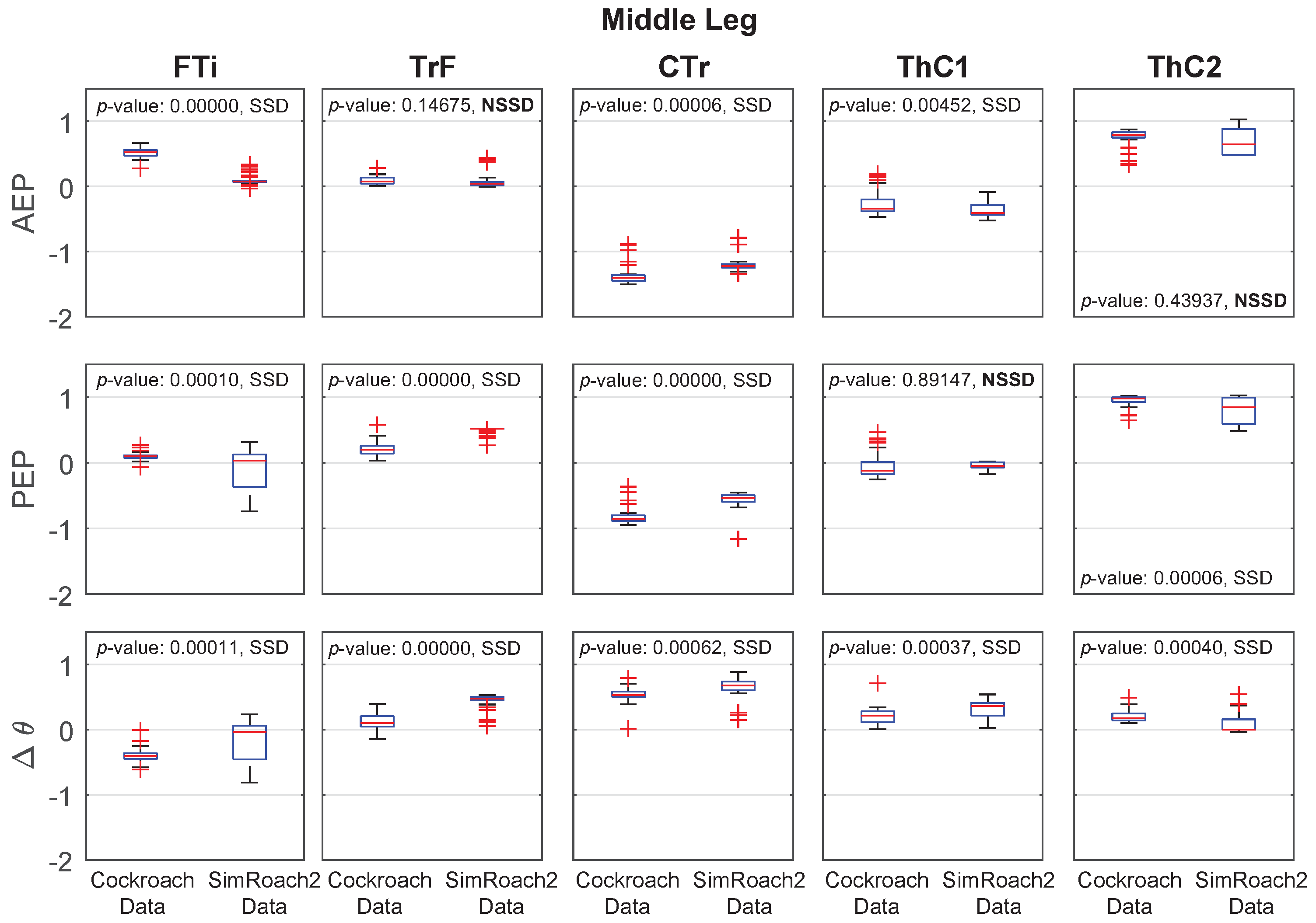
Figure 14.
Hind leg anterior extreme position (AEP), posterior extreme position (PEP), and joint angle data in a cockroach and in SimRoach2. Twenty nine cockroach data points were used. Forty five SimRoach2 data points were used. p-values from the two-sample t-tests and whether there is a statistically-significant difference (SSD, bad match) or no statistically-significant difference (NSSD, good match) between the samples are provided.

Figure 15.
Inter-leg influences result in a stable tripod gait. Data presented over one second of walking. Black bars indicate stance phase.
Figure 15.
Inter-leg influences result in a stable tripod gait. Data presented over one second of walking. Black bars indicate stance phase.

Table 1.
Actuated joints in each leg starting from the joint closest to the body and moving distally outward. Thorax-coxa (ThC) joints act between the thorax and the coxa. Coxa-trochanter (CTr) joints act between the coxa and the trochanter. Trochanter-feumr (TrF) joints act between the trochanter and the femur. Femur-tibia (FTi) joints act between the femur and the tibia.
| Actuated Joints | ||
|---|---|---|
| Front Leg | Middle Leg | Hind Leg |
| ThC2 | ThC2 | ThC2 |
| ThC1 | ThC1 | ThC1 |
| ThC3 | CTr | CTr |
| CTr | TrF | TrF |
| FTi | FTi | FTi |
Table 2.
Summary of inter-leg influences.
| Influence Number | Direction of Influence | Effect of Influence |
|---|---|---|
| Influence 1 | Rostral | Inhibits the start of swing phase when the posterior leg is in its swing phase |
| Influence 2 | Rostral and contralateral | Excites the start of swing phase when the posterior leg enters its stance phase |
| Influence 3 | Caudal and contralateral | Excites the start of swing phase while the anterior leg is in its stance phase, increasing in strength over time |
© 2017 by the authors. Licensee MDPI, Basel, Switzerland. This article is an open access article distributed under the terms and conditions of the Creative Commons Attribution (CC BY) license (http://creativecommons.org/licenses/by/4.0/).
Share and Cite
MDPI and ACS Style
Rubeo, S.; Szczecinski, N.; Quinn, R. A Synthetic Nervous System Controls a Simulated Cockroach. Appl. Sci. 2018, 8, 6. https://doi.org/10.3390/app8010006
AMA Style
Rubeo S, Szczecinski N, Quinn R. A Synthetic Nervous System Controls a Simulated Cockroach. Applied Sciences. 2018; 8(1):6. https://doi.org/10.3390/app8010006
Chicago/Turabian StyleRubeo, Scott, Nicholas Szczecinski, and Roger Quinn. 2018. "A Synthetic Nervous System Controls a Simulated Cockroach" Applied Sciences 8, no. 1: 6. https://doi.org/10.3390/app8010006
Note that from the first issue of 2016, this journal uses article numbers instead of page numbers. See further details here.