Ab Initio Simulation of Attosecond Transient Absorption Spectroscopy in Two-Dimensional Materials

Abstract

We extend the first-principles analysis of attosecond transient absorption spectroscopy to two-dimensional materials. As an example of two-dimensional materials, we apply the analysis to monolayer hexagonal boron nitride (h-BN) and compute its transient optical properties under intense few-cycle infrared laser pulses. Nonadiabatic features are observed in the computed transient absorption spectra. To elucidate the microscopic origin of these features, we analyze the electronic structure of h-BN with density functional theory and investigate the dynamics of specific energy bands with a simple two-band model. Finally, we find that laser-induced intraband transitions play a significant role in the transient absorption even for the two-dimensional material and that the nonadiabatic features are induced by the dynamical Franz–Keldysh effect with an anomalous band dispersion.

1. Introduction

Attosecond transient absorption spectroscopy (ATAS) is a technique that employs attosecond laser pulses to probe modifications to the optical absorption in the time domain. Because its attosecond time-resolution is shorter than a typical time-scale of electron dynamics, which is on the order of femtosecond, it can naturally capture ultrafast electron dynamics in matter. Therefore, ATAS is one of the key experimental techniques to explore ultrafast phenomena where nonlinear electron dynamics play a significant role. Indeed, ATAS has been extensively applied to atoms and molecules over the past decade to investigate ultrafast electron dynamics in such relatively small systems [1,2,3,4,5,6,7]. Recently, ATAS has been further extended to solid-state materials to investigate rather complex electron dynamics in various phenomena such as band-gap renormalization [8], petahertz optical drive [9], dynamical Franz–Keldysh effect [10], photocarrier relaxation [11], exciton dynamics [12] as well as photocarrier injection [13].

Two-dimensional (2D) materials have been attracting great interest from both fundamental and technological points of view because of their remarkable properties. For example, graphene-like 2D materials such as hexagonal boron-nitride (h-BN) have been intensively studied for applications in optelectronic devices and energy storage among others [14,15,16]. Transition metal dichalcogenides (TMDs), another kind of 2D materials, are also attracting attention because of their interesting properties deriving from strong spin-orbit coupling and a large direct-bandgap [16,17,18]. Thanks to recent development of laser technologies, laser-induced ultrafast electron dynamics in such 2D materials has been intensively studied both experimentally and theoretically [19,20,21,22,23,24,25]. For example, the high-order harmonic generation was recently studied in 2D materials [26,27,28,29]. Surprisingly, it was demonstrated that elliptically polarized light can enhance the high-order harmonic generation in graphene [26].

In order to fully understand such laser-induced ultrafast electron dynamics, ATAS is one of the most desirable experimental techniques as it can resolve the dynamics with natural time-resolution. While ATAS for solid-state materials provides a wealth of information on microscopic electron dynamics in materials, the resulting experimental data are often very complicated due to complex electronic structure and highly-nonlinear effects in the dynamics. Therefore, it is hard to directly interpret the experimental results. Ab initio simulation based on the time-dependent density functional theory (TDDFT) [30] is a powerful tool to describe such complex electron dynamics and to provide microscopic insight into the phenomena. Indeed, ab initio TDDFT simulations have been applied to ATAS experiments for solid-state systems and played a significant role to construct the interpretation [8,10,11,13].

Likewise, experimental results of ATAS for 2D materials are expected to be rather complicated. Therefore, ab initio TDDFT simulations are a good candidate to analyze ATAS for 2D materials. To realize such simulation methods, we extend the TDDFT pump–probe simulation [31] of transient absorption spectroscopy to 2D materials. To demonstrate the ab initio ATAS simulation, we employ monolayer h-BN as an example of a 2D material and investigate its transient optical property under intense infrared (IR) laser pulses. Because monolayer h-BN has a large band-gap among many 2D materials, ATAS for h-BN can be investigated in terms of knowledge from the recent ATAS experiments for bulk semiconductor materials [8,10,13]. Furthermore, we analyze the obtained transient absorption spectra of h-BN with a 2D parabolic two-band model and clarify the microscopic mechanism of the ultrafast modification of the optical property.

This paper is organized as follows: in Section 2, we first describe the electron dynamics simulation based on TDDFT. Then, we further describe the linear response calculation and the pump–probe simulation to compute static and transient absorption properties, respectively. In Section 3, we apply the TDDFT pump–probe simulation to monolayer h-BN and investigate its transient optical properties. Furthermore, we analyze the obtained transient absorption spectra with a parabolic two-band model. Finally, our findings are summarized in Section 4.

2. Methods

In this section, we describe our theoretical and numerical methods to simulate ATAS for 2D materials. As an example of 2D materials, we choose monolayer h-BN in this work.

2.1. Electron Dynamics Simulation for Periodic Systems

First, we briefly describe the first-principles electron dynamics simulation based on TDDFT [30]. Details of the simulation are described elsewhere [32]. In the framework of TDDFT, electron dynamics in a periodic system is described by the following time-dependent Kohn–Sham equation,

$$\begin{array}{ccc}\hfill i\hslash \frac{\partial }{\partial t}{u}_{b\overrightarrow{k}}(\overrightarrow{r},t)& =& \left[\frac{1}{2m_e}{\left\{\overrightarrow{p}+\hslash \overrightarrow{k}+\frac{e}{c}\overrightarrow{A}\left(t\right)\right\}}^2+{\widehat{v}}_{ion}+v_H(\overrightarrow{r},t)+v_{XC}(\overrightarrow{r},t)\right]u_{b\overrightarrow{k}}(\overrightarrow{r},t)\hfill \\ & =& H_{KS,\overrightarrow{k}}\left(t\right)u_{b\overrightarrow{k}}(\overrightarrow{r},t),\hfill \end{array}$$

(1)

where $u_{b\overrightarrow{k}}(\overrightarrow{r},t)$ is the Kohn–Sham Bloch wavefunction, b is a band index, and $\overrightarrow{k}$ is the Bloch wave vector. The electron–ion interaction is described by the ionic potential ${\widehat{v}}_{ion}$, while the electron–electron interaction is described by the combination of the Hartree potential $v_H(\overrightarrow{r},t)$ and the exchange–correlation potential $v_{XC}(\overrightarrow{r},t)$. The Hartree potential satisfies the Poisson equation, ${\nabla }^2{v}_H(\overrightarrow{r},t)=4e^2\pi \rho (\overrightarrow{r},t)$, where the electron density $\rho (\overrightarrow{r},t)$ is evaluated as

$$\begin{array}{c}\hfill \rho (\overrightarrow{r},t)=\sum _{b\overrightarrow{k}}{n}_{b\overrightarrow{k}}{\left|u_{b\overrightarrow{k}}(\overrightarrow{r},t)\right|}^2,\end{array}$$

(2)

with occupation factors, $n_{b\overrightarrow{k}}$.

The exchange–correlation potential $v_{XC}(\overrightarrow{r},t)$ is a functional of the electron density. Because its exact form is unknown, one has to approximate it. In this work, we employ the adiabatic local-density approximation [33] (ALDA), where the exchange–correlation potential depends on the electron density locally in space and time. External laser fields are described by spatially-uniform time-varying vector potentials $\overrightarrow{A}\left(t\right)$ in the dipole approximation.

To describe monolayer h-BN, we employ three-dimensional periodic boundary conditions with a hexagonal lattice. The real-space atomic configuration in the plane is shown in Figure 1a. In this work, the y-axis is taken to be parallel to a B-N bond, while the x-axis is taken to be perpendicular to it. The lattice constant of the hexagonal lattice is set to $a=4.76$ a.u. The out-of-plane direction is assigned to the z-axis, and the period of that direction is set to $L=50$ a.u., which is large enough to avoid spurious inter-layer interactions.

We discretize the hexagonal lattice into three-dimensional real-space grid points with a grid spacing about 0.36 a.u. We further discretize the two-dimensional first Brillouin zone of h-BN into $32\times 32$ k-points.

In this work, dynamics of core electrons in the $1s$ shell of Boron and Nitrogen atoms are not expected to be significant for transient absorption. Therefore, we treat explicitly only valence electrons while the core electrons are frozen. For this purpose, we employ the Hartwigsen–Goedecker–Hutter pseudopotentials [34] to describe interactions between valence electrons and ionic cores.

All the density functional theory (DFT) and TDDFT calculations in this work are carried out with the Octopus code [35].

2.2. Optical Property from Linear Response Calculation

Here, we revisit the linear response calculation in time domain to obtain optical properties of 2D materials. For this purpose, we consider electron dynamics in monolayer h-BN under an impulsive perturbation, $\overrightarrow{E}\left(t\right)={\overrightarrow{e}}_x{k}_0\delta \left(t\right)$. The polarization of the perturbation is set along the x-direction in Figure 1a, which is an in-plane direction. The strength of the perturbation $k_0$ is set to 0.005 a.u., which is weak enough to only create excitations on the linear response regime.

In this context, one of the most useful results of TDDFT calculations for 2D materials is the surface density of the electric current:

$$\begin{array}{c}\hfill \overrightarrow{J}\left(t\right)=-\frac{e}{S}\sum _{b\overrightarrow{k}}{n}_{b\overrightarrow{k}}{\int }_{cell}d\overrightarrow{r}{u}_{b\overrightarrow{k}}^{*}(\overrightarrow{r},t){\overrightarrow{v}}_{\overrightarrow{k}}\left(t\right)u_{b\overrightarrow{k}}(\overrightarrow{r},t),\end{array}$$

(3)

where S is the area of the h-BN sheet in the simulation cell, and ${\overrightarrow{v}}_{\overrightarrow{k}}$ is the velocity operator:

$$\begin{array}{c}\hfill {\overrightarrow{v}}_{\overrightarrow{k}}\left(t\right)=\frac{\left[\overrightarrow{r},H_{KS,\overrightarrow{k}}\left(t\right)\right]}{i\hslash }=\frac{1}{m_e}\left[\overrightarrow{p}+\hslash \overrightarrow{k}+\frac{e}{c}\overrightarrow{A}\left(t\right)\right]+\frac{\left[\overrightarrow{r},{\widehat{v}}_{ion}\right]}{i\hslash }.\end{array}$$

(4)

Note that the velocity operator contains a contribution from the ionic potential ${\widehat{v}}_{ion}$ because of the nonlocality of the pseudopotential, which is not commutative with the position operator $\overrightarrow{r}$ [32].

Figure 1b shows the surface current density, $J\left(t\right)$, for the x-direction as a function of time. Since the impulsive distortion is applied at $t=0$, the current is suddenly induced at that time. Then, the induced current shows oscillatory behavior with damping.

One can extract the optical conductivity from the computed current in time domain. The diagonal element of the conductivity can be evaluated as

$$\begin{array}{c}\hfill \sigma \left(\omega \right)=\frac{\int dtJ\left(t\right)e^{i\omega t-\gamma t}}{\int dtE\left(t\right)e^{i\omega t-\gamma t}},\end{array}$$

(5)

where $J\left(t\right)$ and $E\left(t\right)$ are the electric current and the electric field for the polarization direction of the impulsive distortion, respectively. To reduce numerical error due to the finite time propagation in the Fourier transform of Equation (5), we employed a damping factor $\gamma$ of 0.5 eV$/\hslash$.

Figure 1c shows the real part of the optical conductivity of h-BN for the in-plane direction, which is computed from the current in Figure 1b. The computed conductivity shows two peaks at around 5 eV and 15 eV. This double-peak structure is consistent with the previous theoretical work based on the first-principles simulation [36]. Because the real-part of the conductivity is closely related to the optical absorption, we treat it as a direct measure of the photo-absorption in this work. We note that the present calculation with ALDA does not properly describe the excitonic effect which is significant in the optical absorption of h-BN around the optical gap [37,38]. However, as will be shown later, we focus on transitions to conduction states with relatively high energy, where the excitonic effect is expected to be less important. Therefore, we simply ignore the excitonic contribution in this work.

2.3. Transient Optical Properties with Pump–Probe Simulations

Now, we describe the pump–probe simulation to investigate transient optical properties. Details of the numerical pump–probe simulation are described elsewhere [31].

To compute transient optical properties of materials, we consider electron dynamics under pump ${\overrightarrow{E}}_{pump}\left(t\right)$ and probe ${\overrightarrow{E}}_{probe}\left(t\right)$ electric fields. Solving the time-dependent Kohn–Sham Equation (1) under the presence of both the pump and probe fields, one can simulate the electron dynamics induced by the fields. Furthermore, one can calculate the induced electric current by using Equation (3); we shall call the current under both the pump and probe pulses pump–probe current, ${\overrightarrow{J}}_{pump--probe}\left(t\right)$. Additionally, one can simulate electron dynamics under only the pump pulse, and compute the current: we shall call the current induced solely by the pump pulse pump current, ${\overrightarrow{J}}_{pump}\left(t\right)$. To extract the current induced by the probe pulse under the presence of the pump, we define the probe current, ${\overrightarrow{J}}_{probe}\left(t\right)$, as

$$\begin{array}{c}\hfill {\overrightarrow{J}}_{probe}\left(t\right)\equiv {\overrightarrow{J}}_{pump--probe}\left(t\right)-{\overrightarrow{J}}_{pump}\left(t\right).\end{array}$$

(6)

Finally, referring to the above linear response equation, the transient conductivity can be evaluated as

$$\begin{array}{c}\hfill {\sigma }^T(\omega ,T_{probe})=\frac{\int dt{J}_{probe}\left(t\right)e^{i\omega t-\gamma t}}{\int dt{E}_{probe}\left(t\right)e^{i\omega t-\gamma t}},\end{array}$$

(7)

where $T_{probe}$ is the central time of the probe pulse. In contrast to the linear response calculation in equilibrium, the transient conductivity under the pump pulse depends also on the central time of the probe pulse since the time translation symmetry is broken by the pump. Thus, one may investigate dynamics of transient optical properties in time domain by changing the time delay between pump and probe pulses.

To practically carry out the pump–probe simulations, we employ a pump vector potential of the following form:

$$\begin{array}{ccc}\hfill {\overrightarrow{A}}_{pump}\left(t\right)& =& -\frac{c{\overrightarrow{E}}_{pump}}{{\omega }_{pump}}{cos}^2\left(\pi \frac{t}{T_{pump}}\right)sin\left({\omega }_{pump}t\right)\hfill \end{array}$$

(8)

in the domain $(-T_{pump}/2<t<T_{pump}/2)$ and zero outside of it. Here, ${\overrightarrow{E}}_{pump}$ is the peak electric field, ${\omega }_{pump}$ is the mean frequency, and $T_{pump}$ is the full duration of the pump pulse.

To perform the pump–probe simulation, we also employ a similar form for the probe vector potential:

$$\begin{array}{ccc}\hfill {\overrightarrow{A}}_{probe}\left(t\right)& =& -\frac{c{\overrightarrow{E}}_{probe}}{{\omega }_{probe}}{cos}^4\left(\pi \frac{t-T_{delay}}{T_{probe}}\right)sin\left[{\omega }_{pump}\left(t-T_{delay}\right)\right]\hfill \end{array}$$

(9)

in the domain $(-T_{probe}/2<t-T_{delay}<T_{probe}/2)$ and zero outside of it. Here, ${\overrightarrow{E}}_{probe}$ is the peak electric field, ${\omega }_{probe}$ is the mean frequency, and $T_{probe}$ is the full duration of the probe pulse. The time delay between pump and probe pulses is expressed by $T_{delay}$.

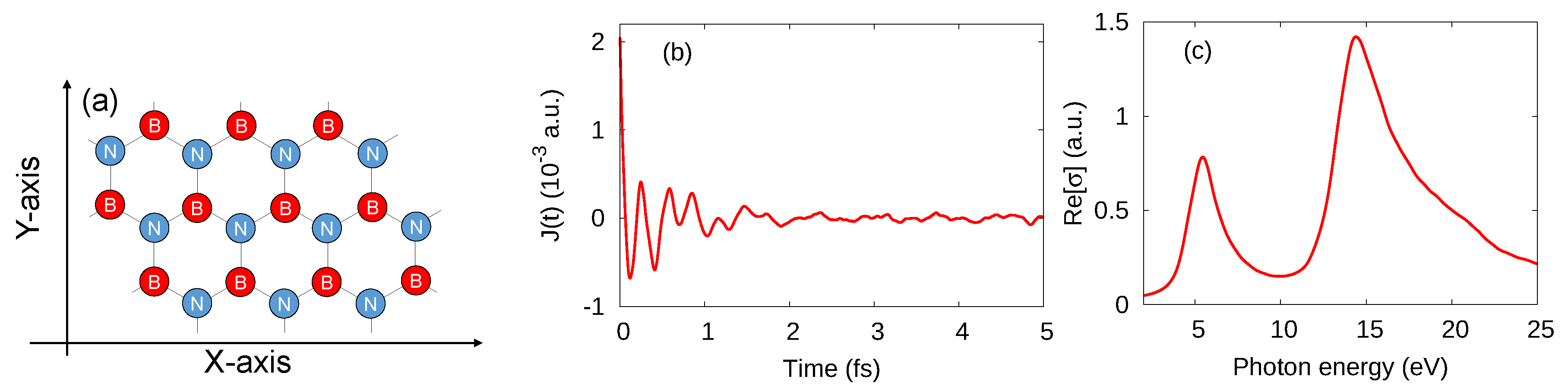
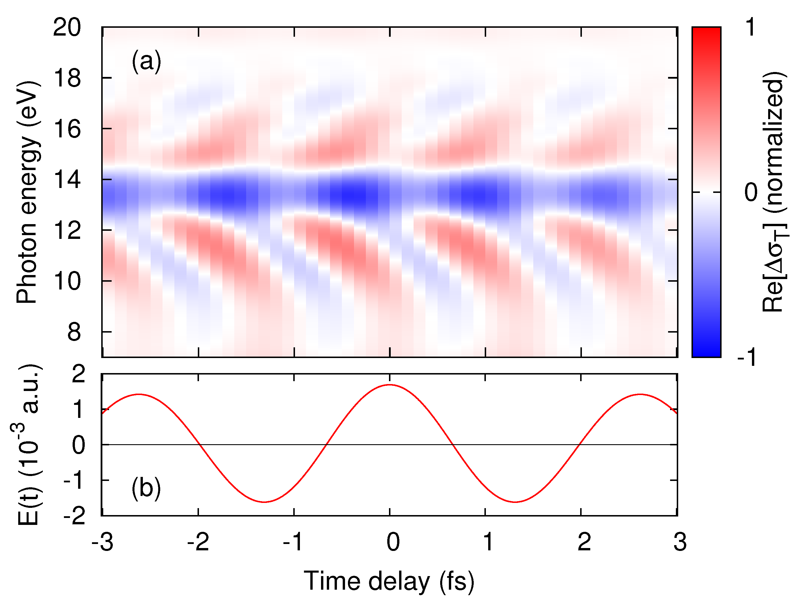
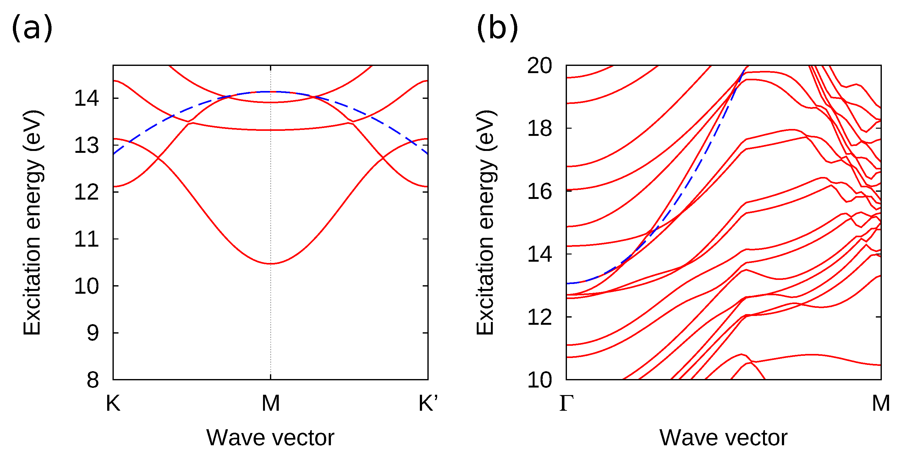
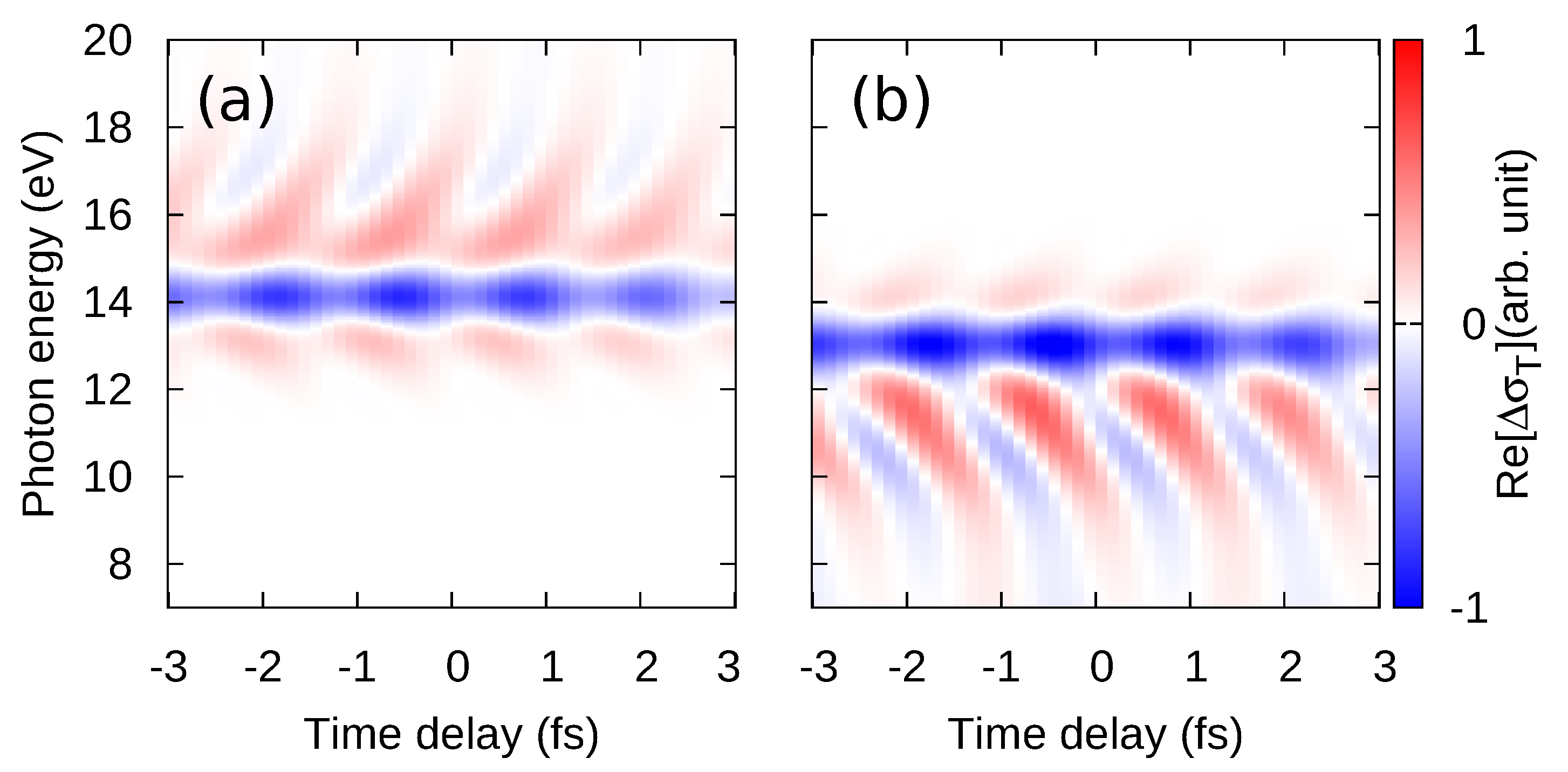
3. Attosecond Transient Absorption of Monolayer h-BN

In this section, we investigate transient optical properties of monolayer h-BN under intense IR pulses. For this purpose, we employ the TDDFT pump–probe approach explained in Section 2.

For the pump–probe simulation, we first set the polarization direction of both the pump and probe pulses to the x-direction in Figure 1a. Thus, the polarization direction of the pump and probe pulses is perpendicular to a B-N bond. Note that h-BN has inversion symmetry along this direction. For the pump pulse, the peak field strength $|{\overrightarrow{E}}_{pump}|$ is set to $8.7\times {10}^8$ V/m, the mean frequency ${\omega }_{pump}$ is set to 1.55 eV$/\hslash$, and the full pulse duration $T_{pump}$ is set to 20 fs. The corresponding full width at half maximum (FWHM) of the pump pulse is about 7.3 fs. For the probe pulse, $|{\overrightarrow{E}}_{probe}|$ is set to $8.7\times {10}^7$ V/m, ${\omega }_{probe}$ is set to 15 eV$/\hslash$, and $T_{probe}$ is set to 1 fs. The corresponding FWHM of the probe pulse is about 260 as. Under these conditions, we repeat the TDDFT pump–probe simulations by changing the pump–probe time-delay, $T_{delay}$.

Figure 2a shows the real-part of the transient conductivity ${\sigma }_T(\omega ,T_{delay})$ computed by the TDDFT pump–probe simulations. The time-profile of the applied pump electric field is also shown in Figure 2b. In Figure 2a, one sees an oscillatory feature with a V-shaped energy dispersion around 15 eV, which we shall call fishbone structure. As seen from the figure, the frequency of the oscillation in time domain is twice that of the pump frequency ${\omega }_{pump}$. The $2{\omega }_{pump}$-oscillation is a direct consequence of the inversion symmetry of the material in the pump–probe direction, which forbids even-order nonlinear responses, because materials with inversion symmetry must show the same response regardless of the sign of the electric field along a symmetry direction. Similar features have been observed in attosecond transient absorption spectroscopy for semiconductors [10,13], and transient terahertz absorption spectroscopy for GaAs quantum wells [39]. These features of bulk materials have been discussed on the basis of the pump-induced intraband transitions and the dynamical Franz–Keldysh effect [40,41]. The dynamical Franz–Keldysh effect is a modification of optical properties of solids under the influence of oscillatory electric fields. It originates from the field-induced intraband transitions via the modification of the dynamical phase factor.

In order to understand the microscopic origin of the fishbone structure in Figure 2, we investigate energies of photo-excited electron-hole pairs based on the independent particle approximation. For this purpose, we compute the vertical excitation energies from the highest valence band to the conduction bands. Note that in the independent particle approximation the transition energy from one state to another is identical to the difference of the single-particle energies of those states, ${ϵ}_{c\overrightarrow{k}}-{ϵ}_{v\overrightarrow{k}}$.

Figure 3 shows the computed vertical transition energies from the highest valence band to the conduction bands at each k point along high symmetry paths through Brillouin zone. Transitions around the M point are described in Figure 3a, while those around the $\Gamma$ point are described in Figure 3b. In Figure 3a, one can see a negative electron-hole mass band around 14 eV at the M point. The negative-mass band is fitted by a parabola (blue-dashed line) to extract band parameters. The extracted reduced electron-hole mass at the M-point is $-3.3m_e$.

Furthermore, we numerically confirmed that all the other vertical transitions in Figure 3a at the M point are dipole forbidden. Therefore, the negative-mass band is expected to have a dominant contribution to the transient absorption spectrum in Figure 2.

To elucidate the contribution from the negative-mass band at the M point, we compute the transient absorption spectrum with a parabolic two-band model. The parabolic two-band model is described in detail elsewhere [42].

In the parabolic two-band model, the electron dynamics at each k point in the Brillouin zone is described by the following Schrödinger equation for two-dimensional state vectors:

$$\begin{array}{c}\hfill i\hslash \frac{d}{dt}\left(\begin{array}{c}{c}_{v\overrightarrow{k}}\left(t\right)\\ c_{c\overrightarrow{k}}\left(t\right)\end{array}\right)=\left(\begin{array}{cc}0& h_{vc,\overrightarrow{k}}\left(t\right)\\ h_{vc,\overrightarrow{k}}^{*}\left(t\right)& 0\end{array}\right)\left(\begin{array}{c}{c}_{v\overrightarrow{k}}\left(t\right)\\ c_{c\overrightarrow{k}}\left(t\right)\end{array}\right),\\ \hfill \end{array}$$

(10)

where the off-diagonal matrix element of the Hamiltonian is given by

$$\begin{array}{c}\hfill h_{vc,\overrightarrow{k}}\left(t\right)=\frac{i{\overrightarrow{p}}_{vc,\overrightarrow{K}\left(t\right)}·{\overrightarrow{E}}_{probe}\left(t\right)}{\Delta {ϵ}_{cv,\overrightarrow{K}\left(t\right)}}\frac{e\hslash }{m}{e}^{\frac{1}{i\hslash }{\int }^{t}d{t}^{\prime }\Delta {ϵ}_{cv,\overrightarrow{K}\left(t^{\prime }\right)}},\end{array}$$

(11)

where $\Delta {ϵ}_{cv,\overrightarrow{k}}$ is the transition energy between the valence and the conduction states at $\overrightarrow{k}$, and ${\overrightarrow{p}}_{vc,\overrightarrow{k}}$ is the transition momentum. In the Hamiltonian matrix, the Bloch wavevector is shifted based on the acceleration theorem, $\overrightarrow{K}\left(t\right)=\overrightarrow{k}+e{\overrightarrow{A}}_{pump}\left(t\right)/\hslash c$, by the pump pulse [43].

Here, in order to elucidate the role of the pump-induced intraband transitions, only the probe electric field ${\overrightarrow{E}}_{probe}\left(t\right)$ is coupled to the transition momentum ${\overrightarrow{p}}_{vc}$, while only the pump vector potential ${\overrightarrow{A}}_{pump}\left(t\right)$ is taken into account in the acceleration theorem. Thus, the probe pulse induces only the interband transitions, while the pump pulse is responsible for intraband transitions.

For this model, we approximate the transition energy by the parabolic band as

$$\begin{array}{c}\hfill \Delta {ϵ}_{cv,\overrightarrow{k}}={ϵ}_g+\frac{{\hslash }^2}{2{\mu }_{eh}}{k}^2,\end{array}$$

(12)

where ${ϵ}_g$ is the band gap, and ${\mu }_{eh}$ is the reduced mass of an electron-hole pair. To describe the negative-mass band at the M point, the reduced mass ${\mu }_{eh}$ is set to ${\mu }_M=-3.3m_e$, and the band gap ${ϵ}_g$ is set to ${ϵ}_{g,M}=14.1$ eV. These parameters are extracted from the parabolic fit shown as the blue-dashed line in in Figure 3.

The negative-mass band causes an artificial crossing of the conduction and the valence bands. To eliminate the effect from the artificial band crossing of the model, we truncate the transition momentum matrix as follows:

$$\begin{array}{c}\hfill p_{vc,\overrightarrow{k}}=\left\{\begin{array}{cc}{p}_{vc},\hfill & ({ϵ}_{g,M}\le \Delta {ϵ}_{cv,\overrightarrow{k}}),\hfill \\ p_{vc}{sin}^2\left(\frac{\pi \Delta {ϵ}_{cv,\overrightarrow{k}}}{2{ϵ}_g}\right),\hfill & (0<\Delta {ϵ}_{cv,\overrightarrow{k}}<{ϵ}_g),\hfill \\ 0,\hfill & \mathrm{otherwise}.\hfill \end{array}\right.\end{array}$$

(13)

Here, the transition momentum at the gap $p_{vc}$ is set to 0.1 a.u. Note that the value of the transition momentum does not affect the structure of absorption spectra as long as the field strength of the probe pulse is weak enough to satisfy the linear response condition.

We apply a pump–probe simulation to the parabolic two-band model and compute the transient absorption spectrum of the negative-mass band. Since the parabolic-band approximation is an appropriate approximation of the electronic structure only around the band edge, we truncate the signal to reduce the contribution from inappropriate regions by applying the following attenuation function to the transient conductivity

$$\begin{array}{c}\hfill w_M\left(\omega \right)=\left\{\begin{array}{cc}1,\hfill & (\omega >{ϵ}_{g,M}/\hslash ),\hfill \\ exp\left[-\frac{1}{2{\sigma }^2}{(\hslash \omega -{ϵ}_{g,M})}^2\right],\hfill & \mathrm{otherwise}.\hfill \end{array}\right.\end{array}$$

(14)

Here, ${ϵ}_{g,M}$ is the corresponding band gap at the M-point, which is 14.1 eV. We set the width of the attenuation $\sigma$ to 1 eV.

Figure 4a shows the truncated transient conductivity, ${\sigma }^T(\omega ,T_{probe})w_M\left(\omega \right)$, of the negative-mass band at the M point. One may see that the transient absorption spectrum of the negative-mass parabolic band model in Figure 4a nicely reproduces the upper-half part of the transient absorption spectrum of the full ab initio simulation in Figure 2. This fact indicates that the upper-half part of the fishbone structure originates from this specific band around the M point, which has the anomalous band dispersion with the negative reduced electron-hole mass.

To reveal the other half contribution in the transient absorption spectrum of h-BN, we investigate vertical transitions around the $\Gamma$ point. Figure 3b shows the vertical transition energies from the highest valence band to conduction bands around the $\Gamma$ point. Among those of transitions around the energy of 13 eV at the $\Gamma$-point, we pick up a single band, which has the largest transition momentum for the polarization direction of the pump and probe pulses. The chosen band is fitted by a parabola that is shown as the blue dashed line in Figure 3b. The extracted band parameters are as follows: the band gap ${ϵ}_g$ is 13.1 eV, and the reduced electron-hole mass ${\mu }_{eh}$ is $1.1m_e$. Employing the parabolic two-band model with these extracted parameters, we computed the transient optical conductivity based on the pump–probe simulation. As explained above, the parabolic fit is only accurate around the band edge. Therefore, we apply the following attenuation function to the transient optical conductivity to reduce the influence from irrelevant energy regions;

$$\begin{array}{c}\hfill w_{\Gamma }\left(\omega \right)=\left\{\begin{array}{cc}1,\hfill & (\omega <{ϵ}_{g,\Gamma }/\hslash ),\hfill \\ exp\left[-\frac{1}{2{\sigma }^2}{(\hslash \omega -{ϵ}_{g,\Gamma })}^2\right],\hfill & \mathrm{otherwise}.\hfill \end{array}\right.\end{array}$$

(15)

Here, ${ϵ}_{g,\Gamma }$ is the corresponding band gap, which is 13.1 eV.

Figure 4b shows the truncated transient conductivity, ${\sigma }^T(\omega ,T_{probe})w_{\Gamma }\left(\omega \right)$, with the parabolic two-band model of the $\Gamma$ point. One can clearly see that the result of the parabolic two-band model in Figure 4b nicely reproduces the half bottom part of the full ab initio simulation result in Figure 2.

To provide the complete description, we combine the results of the two-band models for the M and $\Gamma$ points by simply summing the transient conductivities in Figure 4a,b. The combined transient conductivity is shown in Figure 5. One sees that the combined result nicely reproduces the full ab initio result in the whole investigated photon-energy range. Therefore, we can conclude that the fishbone structure in the transient absorption spectrum of monolayer h-BN consists of two major contributions: One is the contribution from the negative-mass electron-hole band at the M point, accounting for the upper half of the fishbone structure. The other is the contribution from the positive-mass band at the $\Gamma$ point, inducing the lower half of the fishbone structure.

Since the pump-induced interband transitions are completely omitted in the model by construction, the transient absorption of the two-band model in Figure 5 results only from the IR-induced intraband transitions. Therefore, we clearly demonstrated that the IR-induced intraband transitions play crucial roles and the transient absorption is dominated by the dynamical Franz–Keldysh effect even in this 2D material.

Furthermore, based on the decomposition of the transient absorption spectrum in Figure 5 into the contributions from each band in Figure 4a,b, we found that the upper-half part of the transient absorption spectrum of monolayer h-BN originates from the dynamical Franz–Keldysh effect of a specific band around the M point with the anomalous band dispersion, while the lower-half part originates from the conventional dynamical Franz–Keldysh effect with the positive-mass electron-hole band. As intraband motion is often regarded as semi-classical motion of a free particle, the predominant role of intraband motion in the anomalous dispersion has the potential to induce further interesting dynamics in the 2D material.

Finally, we report the transient optical property of monolayer h-BN for a different polarization direction. Here, we set the polarization direction of the pump and probe pulses to the y-axis in Figure 1a. Thus, the polarization direction is parallel to a B-N bond. For this direction, the system does not have the spatial inversion symmetry and it may have even order nonlinear responses. To investigate transient optical properties, we perform pump–probe simulation with the following parameters. For the pump pulse, the peak field strength $|{\overrightarrow{E}}_{pump}|$ is set to $8.7\times {10}^7$ V/m, the mean frequency ${\omega }_{pump}$ is set to 1.55 eV$/\hslash$, and the full pulse-duration $T_{pump}$ is set to 20 fs. For the probe pulse, $|{\overrightarrow{E}}_{probe}|$ is set to $8.7\times {10}^7$ V/m, ${\omega }_{probe}$ is set to 15 eV$/\hslash$, and $T_{probe}$ is set to 1 fs. Under these conditions, we repeat the TDDFT pump–probe simulations by changing the pump–probe time-delay, $T_{delay}$.

Figure 6a shows the computed transient conductivity with the TDDFT pump–probe simulation, and Figure 6b shows the time profile of the applied pump electric field. In contrast to the $2{\omega }_{pump}$-oscillation in Figure 2, which was the consequence of the inversion symmetry, the transient conductivity shows an oscillatory feature with the frequency of ${\omega }_{pump}$ in time domain. The emergence of the ${\omega }_{pump}$-oscillation instead of the $2{\omega }_{pump}$-oscillation is due to the even-order nonlinear responses, which are forbidden for the x-direction due to inversion symmetry.

Despite of the qualitatively different time-domain structures between Figure 2 and Figure 6, both pump–probe configurations show characteristic features in the same photon energy region around 15 eV. According to the above study with the electron-hole pair distribution in Figure 3 and the two-band model analysis, these features might also be related to the anomalous dispersion of the negative-mass electron-hole band around the M point since the photon energy of 15 eV is close to the transition energy of the negative-mass electron-hole pair at the M-point.

Because the two-band model has spatial inversion symmetry and does not have any even-order nonlinearity, the present model is not appropriate to investigate the ${\omega }_{pump}$-oscillation in the spectrum of Figure 6. Therefore, an extension of the model would be required to understand the microscopic mechanism of the ${\omega }_{pump}$-oscillation structure.

4. Conclusions

In this work, we extended the ab initio pump–probe simulation of ATAS for 2D materials in order to provide a platform to understand the microscopic origin of the features observed in ATAS experiments. As an example, we investigated ultrafast modification of optical properties of monolayer h-BN under intense IR pulses.

First, we performed the pump–probe simulations, setting the polarization of the pump and probe pulses along the x-direction in Figure 1a, which is perpendicular to a B-N bond. As a result of the simulation, we obtained the transient absorption spectrum during the laser irradiation. The resulting spectrum presented an oscillatory behavior with a V-shaped energy dispersion: the fishbone structure. The frequency of the oscillatory behavior was found to be twice the frequency of the pump pulse. In previous studies, similar structures have been observed in bulk materials [10,13,39] and understood in terms of the dynamical Franz–Keldysh effect [40,41].

To clarify the microscopic mechanism of the observed transient absorption spectrum of h-BN, we studied the electronic structure of the material with the DFT and found relevant transitions at the M and $\Gamma$ points. To elucidate the contribution from these transitions, we further analyzed the transient absorption spectra with a parabolic two-band model. As a result, we identified that the fishbone structure in Figure 2 consists of two major contributions. One is the dynamical Franz–Keldysh effect around the $\Gamma$ point. The other is also the dynamical Franz–Keldysh effect but with an anomalous band dispersion around the M point. Therefore, we clearly demonstrated that the IR-induced intraband transitions are significant for the transient absorption even in 2D materials. Furthermore, the discovered mechanism based on intraband motion with the anomalous band dispersion indicates the possibility of introducing exotic dynamical properties of the 2D material since the classical analog of the intraband motion in the anomalous dispersion would be a classical motion of a negative mass particle.

Next, we performed the TDDFT pump–probe simulation, setting the polarization of the pump and probe pulses along the y-direction. For this direction, the inversion symmetry of the material is broken, and the system displays even-order nonlinear responses. Indeed, reflecting the nature of the even-order nonlinearity, the obtained transient absorption spectrum shows an oscillation with the frequency of the pump pulse, ${\omega }_{pump}$. Therefore, it was demonstrated that the system presents a qualitatively different behavior for different polarization directions. However, despite the significant differences for the different polarizations in Figure 2 and Figure 6, the characteristic features emerge around the probe photon energy of 15 eV. This fact indicates that the ${\omega }_{pump}$-oscillation structure in the transient absorption spectrum with the y-direction polarization may also be related to the anomalous band dispersion at the M point. In order to understand the microscopic origin of the $\omega$-oscillation structure, an extension of the parabolic two-band model is required.

The demonstrated ab initio ATAS simulation for 2D materials is a very general approach that is applicable not only to single-layered materials but also to multi-layered systems including heterostructures. Here, the interplay of multi-layer and interface effects with geometrical tilting, such as moiré patterns, could strongly affect the electron dynamics and be observed in the time domain.

References

1. Goulielmakis, E.; Loh, Z.H.; Wirth, A.; Santra, R.; Rohringer, N.; Yakovlev, V.S.; Zherebtsov, S.; Pfeifer, T.; Azzeer, A.M.; Kling, M.F.; et al. Real-time observation of valence electron motion. Nature 2010, 466, 739. [Google Scholar] [CrossRef] [PubMed]
2. Wang, H.; Chini, M.; Chen, S.; Zhang, C.H.; He, F.; Cheng, Y.; Wu, Y.; Thumm, U.; Chang, Z. Attosecond Time-Resolved Autoionization of Argon. Phys. Rev. Lett. 2010, 105, 143002. [Google Scholar] [CrossRef] [PubMed]
3. Holler, M.; Schapper, F.; Gallmann, L.; Keller, U. Attosecond Electron Wave-Packet Interference Observed by Transient Absorption. Phys. Rev. Lett. 2011, 106, 123601. [Google Scholar] [CrossRef] [PubMed]
4. Beck, A.R.; Bernhardt, B.; Warrick, E.R.; Wu, M.; Chen, S.; Gaarde, M.B.; Schafer, K.J.; Neumark, D.M.; Leone, S.R. Attosecond transient absorption probing of electronic superpositions of bound states in neon: Detection of quantum beats. New J. Phys. 2014, 16, 113016. [Google Scholar] [CrossRef]
5. Warrick, E.R.; Cao, W.; Neumark, D.M.; Leone, S.R. Probing the dynamics of Rydberg and valence states of molecular nitrogen with attosecond transient absorption spectroscopy. J. Phys. Chem. A 2016, 120, 3165–3174. [Google Scholar] [CrossRef] [PubMed]
6. Reduzzi, M.; Chu, W.C.; Feng, C.; Dubrouil, A.; Hummert, J.; Calegari, F.; Frassetto, F.; Poletto, L.; Kornilov, O.; Nisoli, M.; et al. Observation of autoionization dynamics and sub-cycle quantum beating in electronic molecular wave packets. J. Phys. B At. Mol. Opt. Phys. 2016, 49, 065102. [Google Scholar] [CrossRef] [Green Version]
7. Chew, A.; Douguet, N.; Cariker, C.; Li, J.; Lindroth, E.; Ren, X.; Yin, Y.; Argenti, L.; Hill, W.T.; Chang, Z. Attosecond transient absorption spectrum of argon at the L2,3 edge. Phys. Rev. A 2018, 97, 031407. [Google Scholar] [CrossRef]
8. Schultze, M.; Ramasesha, K.; Pemmaraju, C.; Sato, S.; Whitmore, D.; Gandman, A.; Prell, J.S.; Borja, L.J.; Prendergast, D.; Yabana, K.; et al. Attosecond band-gap dynamics in silicon. Science 2014, 346, 1348–1352. [Google Scholar] [CrossRef] [PubMed]
9. Mashiko, H.; Oguri, K.; Yamaguchi, T.; Suda, A.; Gotoh, H. Petahertz optical drive with wide-bandgap semiconductor. Nat. Phys. 2016, 12, 741. [Google Scholar] [CrossRef]
10. Lucchini, M.; Sato, S.A.; Ludwig, A.; Herrmann, J.; Volkov, M.; Kasmi, L.; Shinohara, Y.; Yabana, K.; Gallmann, L.; Keller, U. Attosecond dynamical Franz–Keldysh effect in polycrystalline diamond. Science 2016, 353, 916–919. [Google Scholar] [CrossRef] [PubMed]
11. Zürch, M.; Chang, H.T.; Borja, L.J.; Kraus, P.M.; Cushing, S.K.; Gandman, A.; Kaplan, C.J.; Oh, M.H.; Prell, J.S.; Prendergast, D.; et al. Direct and simultaneous observation of ultrafast electron and hole dynamics in germanium. Nat. Commun. 2017, 8, 15734. [Google Scholar] [CrossRef] [PubMed] [Green Version]
12. Moulet, A.; Bertrand, J.B.; Klostermann, T.; Guggenmos, A.; Karpowicz, N.; Goulielmakis, E. Soft x-ray excitonics. Science 2017, 357, 1134–1138. [Google Scholar] [CrossRef] [PubMed]
13. Schlaepfer, F.; Lucchini, M.; Sato, S.A.; Volkov, M.; Kasmi, L.; Hartmann, N.; Rubio, A.; Gallmann, L.; Keller, U. Attosecond optical-field-enhanced carrier injection into the GaAs conduction band. Nat. Phys. 2018, 14, 560–564. [Google Scholar] [CrossRef] [Green Version]
14. Castro Neto, A.H.; Guinea, F.; Peres, N.M.R.; Novoselov, K.S.; Geim, A.K. The electronic properties of graphene. Rev. Mod. Phys. 2009, 81, 109–162. [Google Scholar] [CrossRef] [Green Version]
15. Wang, J.; Ma, F.; Sun, M. Graphene, hexagonal boron nitride, and their heterostructures: Properties and applications. RSC Adv. 2017, 7, 16801–16822. [Google Scholar] [CrossRef]
16. Tan, C.; Cao, X.; Wu, X.J.; He, Q.; Yang, J.; Zhang, X.; Chen, J.; Zhao, W.; Han, S.; Nam, G.H.; et al. Recent Advances in Ultrathin Two-Dimensional Nanomaterials. Chem. Rev. 2017, 117, 6225–6331. [Google Scholar] [CrossRef] [PubMed]
17. Wang, Q.H.; Kalantar-Zadeh, K.; Kis, A.; Coleman, J.N.; Strano, M.S. Electronics and optoelectronics of two-dimensional transition metal dichalcogenides. Nat. Nanotechnol. 2012, 7, 699. [Google Scholar] [CrossRef] [PubMed]
18. Manzeli, S.; Ovchinnikov, D.; Pasquier, D.; Yazyev, O.V.; Kis, A. 2D transition metal dichalcogenides. Nat. Rev. Mater. 2017, 2, 17033. [Google Scholar] [CrossRef]
19. Gierz, I.; Petersen, J.C.; Mitrano, M.; Cacho, C.; Turcu, I.C.E.; Springate, E.; Stöhr, A.; Köhler, A.; Starke, U.; Cavalleri, A. Snapshots of non-equilibrium Dirac carrier distributions in graphene. Nat. Mater. 2013, 12, 1119. [Google Scholar] [CrossRef] [PubMed]
20. De Giovannini, U.; Hübener, H.; Rubio, A. A First-Principles Time-Dependent Density Functional Theory Framework for Spin and Time-Resolved Angular-Resolved Photoelectron Spectroscopy in Periodic Systems. J. Chem. Theory Comput. 2017, 13, 265–273. [Google Scholar] [CrossRef] [PubMed]
21. Bertoni, R.; Nicholson, C.W.; Waldecker, L.; Hübener, H.; Monney, C.; De Giovannini, U.; Puppin, M.; Hoesch, M.; Springate, E.; Chapman, R.T.; Ernstorfer, R.; et al. Generation and Evolution of Spin-, Valley-, and Layer-Polarized Excited Carriers in Inversion-Symmetric WSe2. Phys. Rev. Lett. 2016, 117, 277201. [Google Scholar] [CrossRef] [PubMed]
22. Shin, D.; Hübener, H.; De Giovannini, U.; Jin, H.; Rubio, A.; Park, N. Phonon-driven spin-Floquet magneto-valleytronics in MoS2. Nat. Commun. 2018, 9, 638. [Google Scholar] [CrossRef] [PubMed]
23. Sentef, M.A.; Claassen, M.; Kemper, A.F.; Moritz, B.; Oka, T.; Freericks, J.K.; Devereaux, T.P. Theory of Floquet band formation and local pseudospin textures in pump–probe photoemission of graphene. Nat. Commun. 2015, 6, 7047. [Google Scholar] [CrossRef] [PubMed]
24. Liu, R.Y.; Ogawa, Y.; Chen, P.; Ozawa, K.; Suzuki, T.; Okada, M.; Someya, T.; Ishida, Y.; Okazaki, K.; Shin, S.; et al. Femtosecond to picosecond transient effects in WSe 2 observed by pump–probe angle-resolved photoemission spectroscopy. Sci. Rep. 2017, 7, 15981. [Google Scholar] [CrossRef] [PubMed]
25. Oka, T.; Aoki, H. Photovoltaic Hall effect in graphene. Phys. Rev. B 2009, 79, 081406. [Google Scholar] [CrossRef] [Green Version]
26. Yoshikawa, N.; Tamaya, T.; Tanaka, K. High-harmonic generation in graphene enhanced by elliptically polarized light excitation. Science 2017, 356, 736–738. [Google Scholar] [CrossRef] [PubMed]
27. Liu, H.; Li, Y.; You, Y.S.; Ghimire, S.; Heinz, T.F.; Reis, D.A. High-harmonic generation from an atomically thin semiconductor. Nat. Phys. 2016, 13, 262. [Google Scholar] [CrossRef]
28. Chizhova, L.A.; Libisch, F.; Burgdörfer, J. High-harmonic generation in graphene: Interband response and the harmonic cutoff. Phys. Rev. B 2017, 95, 085436. [Google Scholar] [CrossRef]
29. Tancogne-Dejean, N.; Rubio, A. Atomic-like high-harmonic generation from two-dimensional materials. Sci. Adv. 2018, 4, eaao5207. [Google Scholar] [CrossRef] [PubMed] [Green Version]
30. Runge, E.; Gross, E.K.U. Density-Functional Theory for Time-Dependent Systems. Phys. Rev. Lett. 1984, 52, 997–1000. [Google Scholar] [CrossRef]
31. Sato, S.A.; Yabana, K.; Shinohara, Y.; Otobe, T.; Bertsch, G.F. Numerical pump–probe experiments of laser-excited silicon in nonequilibrium phase. Phys. Rev. B 2014, 89, 064304. [Google Scholar] [CrossRef]
32. Bertsch, G.F.; Iwata, J.I.; Rubio, A.; Yabana, K. Real-space, real-time method for the dielectric function. Phys. Rev. B 2000, 62, 7998–8002. [Google Scholar] [CrossRef] [Green Version]
33. Perdew, J.P.; Wang, Y. Accurate and simple analytic representation of the electron-gas correlation energy. Phys. Rev. B 1992, 45, 13244–13249. [Google Scholar] [CrossRef]
34. Hartwigsen, C.; Goedecker, S.; Hutter, J. Relativistic separable dual-space Gaussian pseudopotentials from H to Rn. Phys. Rev. B 1998, 58, 3641–3662. [Google Scholar] [CrossRef] [Green Version]
35. Andrade, X.; Strubbe, D.; De Giovannini, U.; Larsen, A.H.; Oliveira, M.J.T.; Alberdi-Rodriguez, J.; Varas, A.; Theophilou, I.; Helbig, N.; Verstraete, M.J.; et al. Real-space grids and the Octopus code as tools for the development of new simulation approaches for electronic systems. Phys. Chem. Chem. Phys. 2015, 17, 31371–31396. [Google Scholar] [CrossRef] [PubMed] [Green Version]
36. Beiranvand, R.; Valedbagi, S. Electronic and optical properties of h-BN nanosheet: A first principles calculation. Diamond Relat. Mater. 2015, 58, 190–195. [Google Scholar] [CrossRef]
37. Wirtz, L.; Marini, A.; Rubio, A. Excitons in Boron Nitride Nanotubes: Dimensionality Effects. Phys. Rev. Lett. 2006, 96, 126104. [Google Scholar] [CrossRef] [PubMed]
38. Cudazzo, P.; Sponza, L.; Giorgetti, C.; Reining, L.; Sottile, F.; Gatti, M. Exciton Band Structure in Two-Dimensional Materials. Phys. Rev. Lett. 2016, 116, 066803. [Google Scholar] [CrossRef] [PubMed]
39. Uchida, K.; Otobe, T.; Mochizuki, T.; Kim, C.; Yoshita, M.; Akiyama, H.; Pfeiffer, L.N.; West, K.W.; Tanaka, K.; Hirori, H. Subcycle Optical Response Caused by a Terahertz Dressed State with Phase-Locked Wave Functions. Phys. Rev. Lett. 2016, 117, 277402. [Google Scholar] [CrossRef] [PubMed] [Green Version]
40. Jauho, A.P.; Johnsen, K. Dynamical Franz–Keldysh Effect. Phys. Rev. Lett. 1996, 76, 4576–4579. [Google Scholar] [CrossRef] [PubMed] [Green Version]
41. Otobe, T.; Shinohara, Y.; Sato, S.A.; Yabana, K. Femtosecond time-resolved dynamical Franz–Keldysh effect. Phys. Rev. B 2016, 93, 045124. [Google Scholar] [CrossRef]
42. Sato, S.A.; Lucchini, M.; Volkov, M.; Schlaepfer, F.; Gallmann, L.; Keller, U.; Rubio, A. Role of intraband transitions in photocarrier generation. Phys. Rev. B 2018, 98, 035202. [Google Scholar] [CrossRef]
43. Houston, W.V. Acceleration of Electrons in a Crystal Lattice. Phys. Rev. 1940, 57, 184–186. [Google Scholar] [CrossRef]
Figure 1. (a) atomic configuration of monolayer h-BN; (b) current density in time domain after the impulsive distortion at t = 0 ; (c) real-part of surface conductivity, σ ( ω ) , of h-BN, calculated by TDDFT with ALDA.
Applsci 08 01777 g001
Figure 2. (a) real part of the transient conductivity of monolayer h-BN under the IR pump pulse for the x-direction in Figure 1a; (b) the time-profile of the applied pump electric field. The result is computed by TDDFT with ALDA.
Applsci 08 01777 g002
Figure 3. Red lines show vertical transition energies from the highest valence band to conduction bands in monolayer h-BN around (a) the M point and (b) the Γ point. The transition energies are computed by the difference of the Kohn–Sham eigenenergies of the highest valence band and conduction bands, ϵ c k - ϵ v k , corresponding to excitations in the independent particle approximation. Blue lines show the parabolic fits of specific bands.
Applsci 08 01777 g003
Figure 4. Transient surface conductivities of parabolic two-band models under the femtosecond IR pulse. The panels (a) and (b) show the result of the parabolic band shown as the blue-dashed line in Figure 3a, b, respectively.
Applsci 08 01777 g004
Figure 5. (a) transient surface conductivities of the combined two-band models at M and Γ points. This result is nothing but the summation of Figure 4a,b; (b) the time-profile of the applied pump electric field.
Applsci 08 01777 g005
Figure 6. (a) real part of the transient conductivity of monolayer h-BN under the IR pump pulse for the y-direction in Figure 1a; (b) the time-profile of the applied pump electric field. The result is computed by TDDFT with ALDA.
Applsci 08 01777 g006