Article

Artificial Neural Network Trained to Predict High-Harmonic Flux

1
National Institute for R&D of Isotopic and Molecular Technologies, Donat str. 67-103, 400293 Cluj-Napoca, Romania
2
Chemical Engineering Department, Babeș-Bolyai University, Arany János str. 11, 400028 Cluj-Napoca, Romania
*
Author to whom correspondence should be addressed.
Appl. Sci. 2018, 8(11), 2106; https://doi.org/10.3390/app8112106
Submission received: 28 September 2018 / Revised: 19 October 2018 / Accepted: 29 October 2018 / Published: 1 November 2018
(This article belongs to the Special Issue Attosecond Science and Technology: Principles and Applications)

Abstract

:

Featured Application

We present a method based on artificial neural networks—as an efficient procedure—aimed to predict the outcome of high-order harmonic generation experiments with previously unexplored parameters. The main goal is to provide quick help for attosecond science laboratories in designing experiments.

Abstract

In this work we present the results obtained with an artificial neural network (ANN) which we trained to predict the expected output of high-order harmonic generation (HHG) process, while exploring a multi-dimensional parameter space. We argue on the utility and efficiency of the ANN model and demonstrate its ability to predict the outcome of HHG simulations. In this case study we present the results for a loose focusing HHG beamline, where the changing parameters are: the laser pulse energy, gas pressure, gas cell position relative to focus and medium length. The physical quantity which we predict here using ANN is directly related to the total harmonic yield in a specified spectral domain (20–40 eV). We discuss the versatility and adaptability of the presented method.

1. Introduction and Motivation

High-order harmonic generation (HHG) is a well-established experimental technique for obtaining coherent radiation in the XUV to soft X-ray spectral domain on the attosecond timescale [1,2]. The process of HHG is highly nonlinear and has very low efficiency [3]. Despite the fact that high-harmonic radiation is the result of the highly nonlinear interaction between the atom and the driving laser pulse, this method is reliable and provides coherent secondary sources in the UV–XUV–soft-X-ray spectral domain with a table-top setup. The ELI-ALPS pan-European research infrastructure is also based on HHG sources [4], demonstrating that the increasing research efforts dedicated to this field are fully justified. Given the advantages of exploring HHG in the emerging field of Attosecond Science and Technology, considerable research effort is being dedicated to find ways for increasing high-harmonic efficiency by implementing either tight [5] or loose focusing configurations [4,6], inventing different quasi-phase-matching techniques [7,8,9,10,11,12,13,14], multi-color and/or multi-jet configurations [12,15,16,17], but also to extend the available photon energy to reach the water-window [17,18,19] region.
Numerical approaches are unavoidable in this research for several reasons: (i) often, new experiments are designed based on predictions resulting from simulations; (ii) interpretation of existing experimental results cannot be done without additional results from models; (iii) when looking for the best possible outcome within given experimental possibilities, reliable simulation tools can considerably contribute in finding the best solution.
Increasing efficiency and/or finding the optimum photon flux obtainable within a restricted parameter space is crucial. Experimental scan along many tunable parameters is very time and resource consuming, additionally the experimental uncertainties result in variations from one measurement to the next. Simulation with a complete 3D model seems a more convenient route. However, as we will show in the following section, scanning along multiple parameters, typically 4–5, implies the execution and interpretation of hundreds to thousands of simulation runs. Since the amount of raw data and computational effort is very difficult to be managed, we propose an additional method to extract the needed information from the data pool, and to predict possible outcomes for parameter combinations which were not included in the original simulation sets.
The need for specialized algorithms capable to perform optimization procedures has been expressed, and evolutionary algorithms have been constructed to achieve this goal, see for example an early review on the adaptive control techniques [20]. Recently, genetic algorithms were used to optimize the optical waveforms [21,22,23] coming from a light-wave synthesizer with the goal either to extend the high-harmonic cutoff or to enhance the high-harmonic efficiency. In this respect, artificial neural networks (ANN) are known to be high speed mathematical models that are capable of solving linear and non-linear multivariate regression problems [24,25], being generally used for their excellent prediction capabilities [26,27] but also for their capacity to solve problems such as classification [28,29], pattern recognition [30] or system control [31,32,33]. Inspired by the human brain, these numerical modelling techniques are able to gain high efficiency and accuracy in the presence of uncertainties due to their ability to learn from experience [34]. Based on these properties and also on their effectiveness in processing large amount of data, the ANNs have applicability in various fields such as medicine [35], engineering [36,37], science technology [38], nanotechnology [39,40] or physics [41].
In this particular paper the physical quantity we want to predict is the total harmonic flux in a predefined spectral region of the high-harmonic spectrum, which we define as yield:
Y = ω 1 ω 2 0 R [ E h ( ω , r ) ] 2 r d r d ω ,
where [ω1; ω2] is the spectral domain of interest, R is the radial extent of the interaction region, Eh(ω,r) is the harmonic field in spectral representation.
Alternatively, one can identify different physical quantities which we want to predict using ANN, for example the existence and bandwidth/duration of isolated attosecond pulses. One can search to maximize the brightness of a single harmonic as the function of different experimental parameters, as it has already been done experimentally [42].
We propose here a combined method to predict the photon flux in the 20–40 eV spectral range while varying four experimental parameters: laser pulse energy, gas pressure, gas cell position and medium length. For this prediction an artificial neural network is designed, trained and tested. The input data are the results obtained with the 3D non-adiabatic model (see next section) from a 4-dimensional parameter scan [43].
The paper has the following structure: in Section 2.1 we briefly describe the 3D non-adiabatic model for laser pulse propagation and high-harmonic generation, while in Section 2.2 the artificial neural network method is presented. In Section 3 we present and discuss the results obtained with the ANN, we test its robustness and reliability. Possible applications are suggested as well since the major role of this prediction procedure is to provide a quick help for HHG laboratories: predict the expected outcome of HHG experiments to be performed with previously unexplored experimental parameter combinations.

2. Theoretical Models and Numerical Methods for High-Harmonic Generation and Artificial Neural Networks

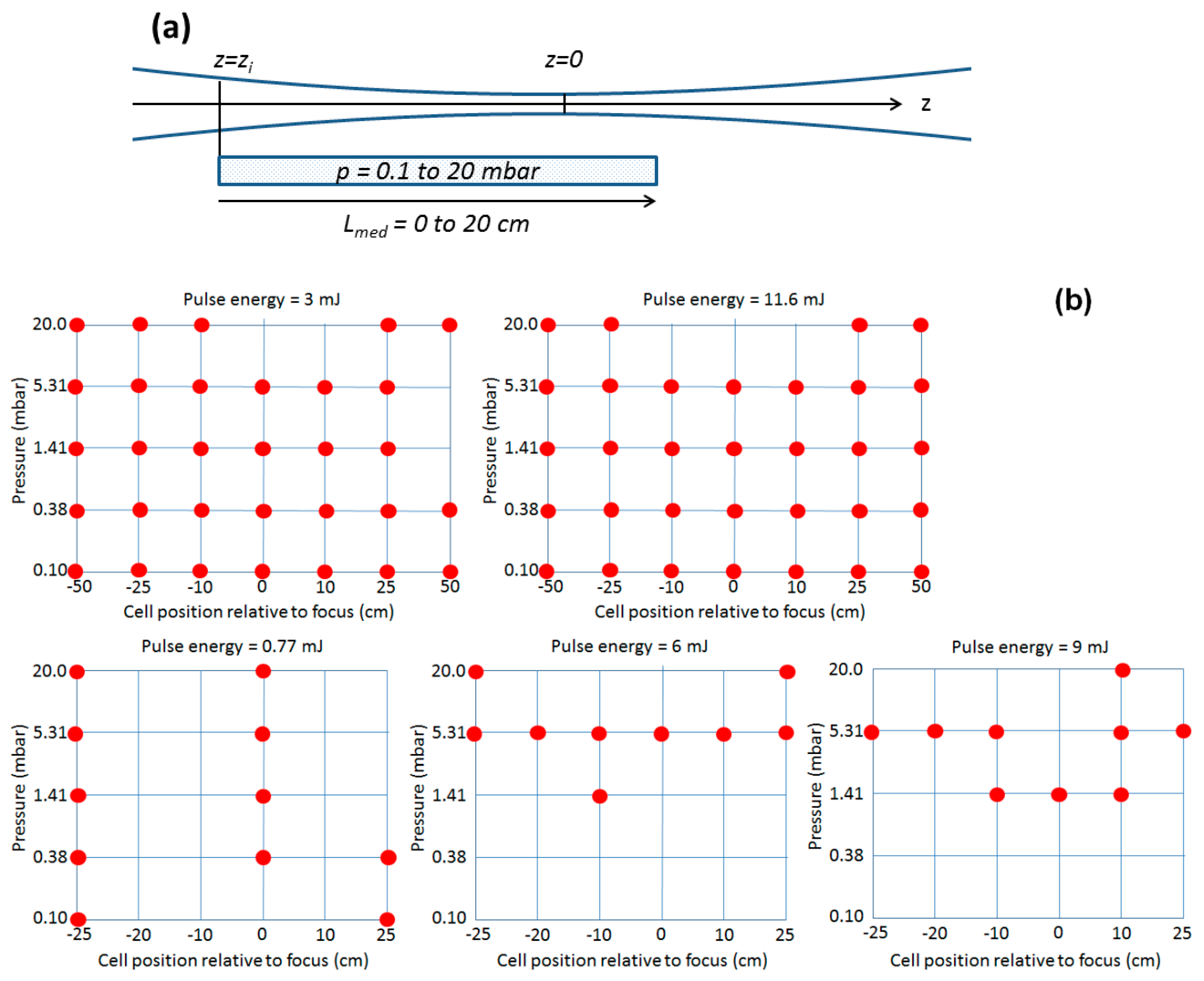
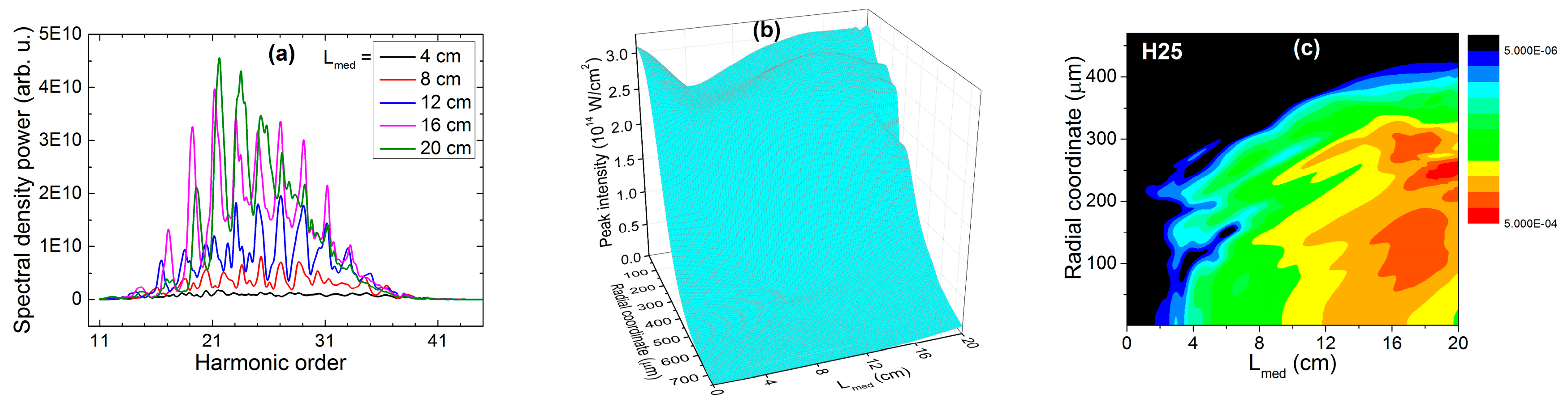
2.1. High-Harmonic Generation

In order to have sufficient input data for the training of the ANN, extensive simulation of the complete HHG process has been performed using a 3D non-adiabatic model [44] while the theoretical basis implemented in the simulation code has been described in [45]. According to the physical reality, this model has three main parts: (A) solves the propagation equation of the fundamental laser pulse in the generating medium, which is a noble gas in our case; (B) quantify the response of the individual atoms to the external laser electric field; and (C) solves the propagation equation of the dipole radiation generated in step (B) within the same medium.
(A) The propagation equation for the fundamental laser pulse is the Maxwell wave equation. This is solved with a self-consistent iterative method in frequency domain and using the paraxial approximation. The method is implemented in a way that the full electric field (carrier and envelope) is calculated, without using the slowly varying envelope approximation. The interaction configuration is considered to have cylindrical symmetry around the propagation direction defined as z axis, and r the radial coordinate. The pulse experiences an effective refractive index—function of time and spatial coordinates—which accounts for the linear refraction and absorption, the intensity-dependent optical Kerr effect and the dispersion due to the free electrons. In this way the modifications of the generating pulse during propagation are included: self-phase modulation, pulse lengthening, intensity clamping, possible self-guiding. The propagation part of the simulation code is partially parallelized. For detailed mathematical formulation we refer to [44].
(B) The elemental interaction of a laser pulse with an atom is treated within the strong-field approximation and the generated dipole is calculated by solving the Lewenstein integral [46]. This part of the simulation code has been also parallelized, but it is still the most demanding part of the calculation in terms of CPU time and memory use.
(C) The total harmonic field results from the propagation and coherent addition of the atomic polarizations calculated in step (B). The wave equation describing the propagation of the harmonic field is similar to the wave equation for the fundamental, but the source term here is the non-linear polarization calculated in step (B).
This simulation code has several advantages which make it a very useful tool in the design and interpretation of HHG experiments. When we construct one specific case all the needed input data are experimentally measurable (or can be estimated). These are information about the fundamental laser pulse like beam type, pulse energy, duration, carrier-envelope phase, chirp; geometrical arrangement like aperture, focusing, cell position and length, far-field detection configuration; interaction medium like gas type and pressure profile.
One typical full calculation yields a complex set of quantities in the grid points built over the interaction domain such as: laser pulse shape before and after propagation in time and frequency representation, peak intensity and ionization fraction, harmonic spectrum in near- and far-field (spectral domain), harmonic bursts in temporal domain, spatial build-up of selected harmonic orders. The most important outcome is the harmonic power spectrum which can be directly compared to the experimentally measured spectra. In addition, the simulation results provide a detailed insight into the physics of the whole process (laser and harmonic field propagation), at sub-optical-cycle temporal resolution, while phase-matching conditions can be examined as well.
The model is flexible in the sense that it can be modified according to diverse experimental conditions. It has been extended to be able to treat multiple electric fields (two-color [47,48,49,50,51,52,53] and three- or four-color field coming from a light-field synthesizer [22]) or multiple jets configurations. At very high laser intensities the atoms become highly charged ions, therefore we implemented also the multiple ionization scenario [54,55]. Propagation in a fiber is essentially different from free space propagation, therefore this scenario has also been recently introduced. In attosecond laboratories very diverse experimental configurations are tried, for example Airy beams obtained with drilled mirror—also implemented in one version of the code.
The theoretical model implemented in the complete 3D simulation code is suitable for exploring a multi-dimensional parameter space and searching for optimum based on a given criterion. We can search for the maximum harmonic yield in a given spectral domain, or can look for the existence of a single attosecond pulse, or maximum cutoff energy within given parameter ranges. Although such a scan along multiple parameters is possible to be performed also experimentally, this process would require much more resources than usually affordable, therefore it is recommended to perform a scan with computer simulations.
Depending on the complexity of the possible experimental situation to be simulated, one whole calculation typically takes between a few hours to 1–2 days. This estimation is done based on the typical cases implemented so far on a cluster IBM System iDataPlex M4 dx360 (in Data Center of INCDTIM Cluj-Napoca).
When we need to explore an unknown parameter space, and we have to scan along several experimental parameters, the number of cases to be run is on the order of hundreds to thousands. Even though, one can afford only sparse sampling along each parameter. Therefore, if we want to search for an optimum output, for example harmonic yield, this sparse sampling (maximum 5 values for one parameter) is far not enough and cannot guarantee that an optimum configuration can be found. Typically in an experiment the gas pressure for example can be varied continuously.

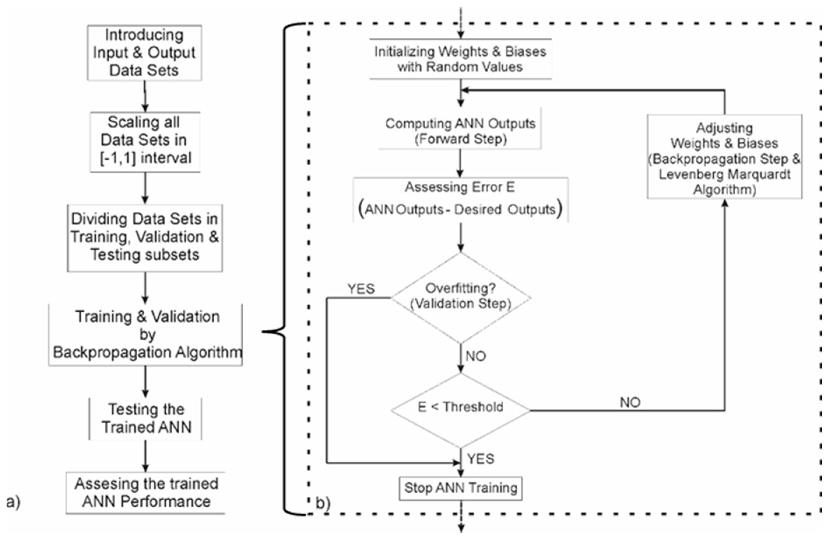
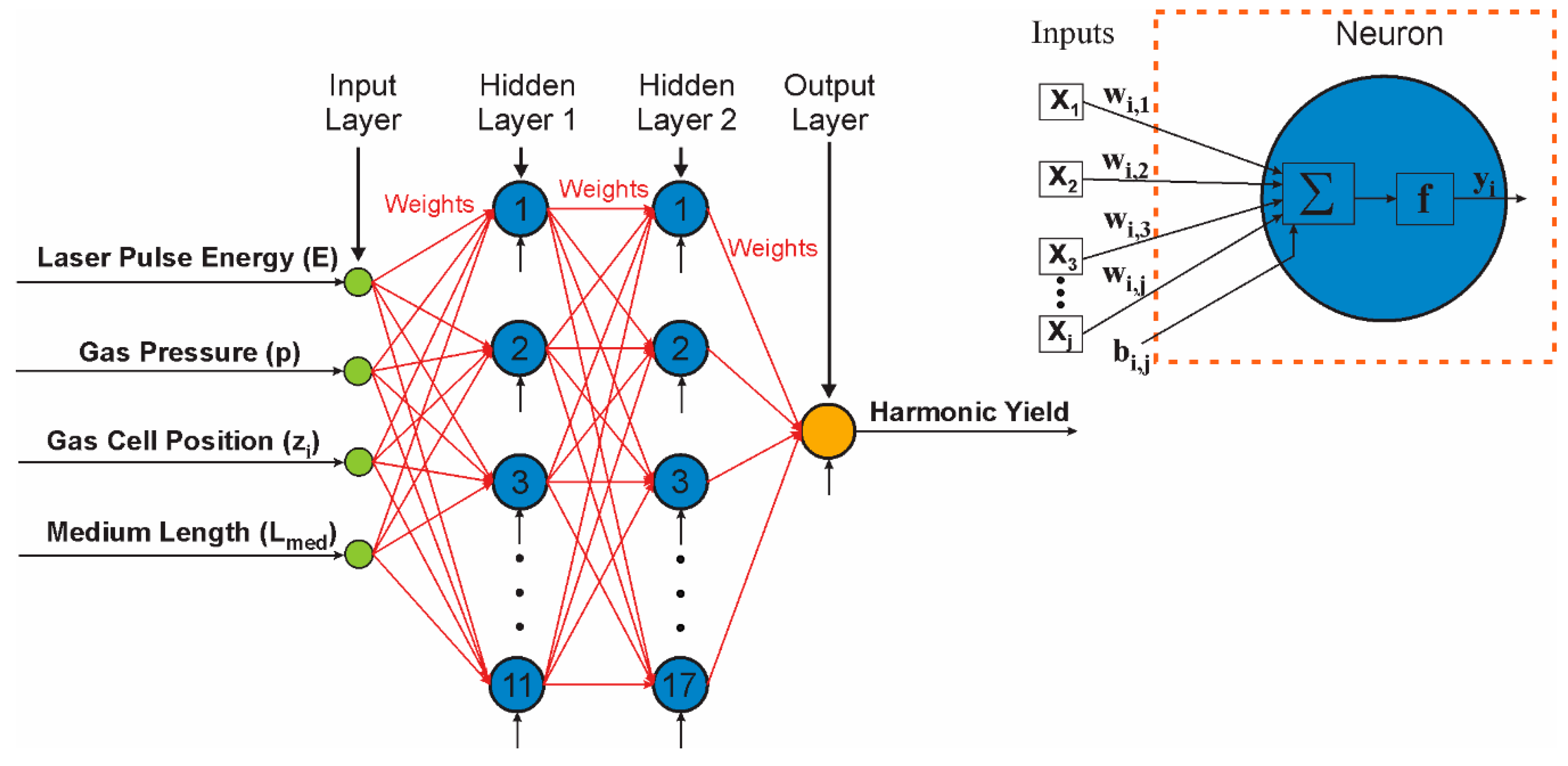
2.2. Artificial Neural Networks

In an ANN, neurons are the ones responsible for processing the information. Each computing unit receives a weighted signal from all the previous neighboring neurons, sums the received signals and its own bias, processes the information via a transfer function and generates the output [27,56]. The neurons are organized in input layer, output layer and one or several hidden layers. As general feature, for prediction purposes, the connections between the neurons that belong to the same layer are not allowed, the information being directed from the input towards the output layer [57,58]. This kind of ANN is named feed-forward neural network and, in most cases, it is associated with the back-propagation learning algorithm [26,59,60].
The main steps performed for training the ANN using the backpropagation algorithm are presented in Figure 1a. Input and desired output data sets are firstly scaled into the [−1, 1] interval for computation accuracy and then divided in training, validation and testing subsets. The backpropagation algorithm, presented in the detail of Figure 1b, iteratively adjusts the weights and biases of the ANN, starting from random values, until the difference between the ANN computed and desired outputs (error) is less than an imposed threshold. In order to avoid overfitting, the validation subset is used to early stop the training procedure. The trained ANN performance is then assessed using the testing data subset, not yet seen by the ANN.
Regarding the HHG process, it is known that the harmonic yield is non-linearly influenced by several parameters such as the fundamental laser pulse characteristics, focusing geometry, gas type and pressure which characterize the medium where HHG takes place. For this particular study we chose as varying parameters the laser pulse energy (E), gas pressure (p), gas cell position (zi) and medium length (Lmed). Consequently, these four process parameters are chosen to be the ANN inputs, whereas the harmonic yield is the model output. Based on the 3D non-adiabatic model, a total number of 453 input-output data sets were obtained and, subsequently, were divided in: (i) training data which represent 77.9% of the total amount of input-output data sets, (ii) validation data (15.7%) and (iii) testing data (6.4%). The testing data subset is obtained by uniformly extracting every sixteenth sample from the initial data. From the remaining data, every sixth sample was extracted to obtain the validation subset, whereas the remaining data represent the training data subset. The higher percentage of the training and validation subsets with respect to the testing subset is explained by the fact that the process is extremely nonlinear and, for good training results, more data are needed for the training and validation steps.
As a result of the complexity of the HHG process, the multilayer feed-forward network is structured in one input layer, two hidden layers and one output layer, the appropriate number of neurons in the hidden layers being found by systematically testing the ANN performance (Figure 2). The information from the hidden and output layers is processed with two different transfer functions: the hidden layer uses a tansigmoid function (Equation (2)) [61], whereas a linear transfer function is applied for the output layer. The ANN is trained with the Levenberg-Marquardt backpropagation algorithm, which is a standard technique for solving nonlinear least square problems [62,63], is included in the backpropagation procedure.
f = 2 1 + exp ( 2 n ) 1
where n is the sums of the neuron received signals and its own bias.
Several networks are trained and the best is chosen such that the ANN performance is maximized. The performance of the model is statistically evaluated using the Pearson correlation factor (R) and the relative errors (RE). Consequently, the best ANN has the highest correlation factor and the lowest relative errors.
R = i = 1 n ( X s i X s ¯ ) ( X A N N i X A N N ¯ ) i = 1 n ( X s i X s ¯ ) 2 i = 1 n ( X A N N i X A N N ¯ ) 2
where Xsi is the simulated output value, XANNi is the model predicted output value, X S ¯ and X A N N ¯ are the arithmetic means of the experimental and respectively, of the predicted output values.
RE = 100 X A N N i X s i X s i

3. Results and Discussion

The main goal of this research is to explore a possible loose focusing HHG configuration and find a combination of input experimental parameters which enable the generation of XUV attosecond pulses at high flux. We have built up one scenario which is experimentally feasible in currently operating large attosecond science facilities, for example the ELI-ALPS. All input parameters are experimentally measurable, from which we fix all but 4 parameters, these are the scanned parameters.
Fixed input data are: pulse duration 10 fs, central wavelength 800 nm, focal length 21 m, radius (1/e2 intensity) of the beam at the focusing element is 30 mm, total length of the interaction region is 20 cm, gas medium is argon. The scanned parameters with the values chosen for the full 3D calculations are the following: input laser pulse energy E (0.77; 3; 6; 9; 11.6) mJ; argon pressure p (0.1; 0.38; 1.41; 5.31; 20) mbar; cell entrance position relative to the nominal focus zi (−50; −25; −20; −10; 0; 10; 25; 50) cm, medium length Lmed (4; 8; 12; 16; 20) cm. Negative values for zi stand for gas cell beginning before the focus position. Although the parameters are very sparsely spaced, scanning along all these parameters and performing complete 3D simulations, while also to individually analyze and interpret the results means an enormous data pool and working time and effort, which would be very inefficient. In Figure 3 we represent in a very schematic manner the general configuration (Figure 3a) and the cases for which the complete 3D simulations have been performed, checked, validated and analyzed (Figure 3b).
The unprecedented power of the ANN comes in exactly at this stage of the research. (1) We set the ranges of all the moving parameters; (2) we perform—in a carefully chosen way—a sufficient number of complete simulations, such as to have representative points from every part of the multi-dimensional parameter space; (3) use these simulation results as inputs for the ANN; (4) train, test and validate the ANN as it was presented in Section 2.2. The expected results are the estimated high-harmonic yields in the whole multi-dimensional parameter space with arbitrarily fine resolution along each parameter. We emphasize that the ANN method in the present stage of implementation is not yet a parameter optimization method, but an efficient prediction method. However, the trained ANN is also suitable to search for optimum, and the maximum yield within this 4-dimensional parameter space can be found by the user.
The results obtained with the complete 3D code are discussed in detail elsewhere [43]. There the main result was that the highest harmonic yield around 40 eV can be obtained with the parameter combination: E = 11.6 mJ; p = 5.31 mbar; zi = −25 cm; Lmed = 16 cm. In this study we also test this result, and present other parameter combinations which guarantee high yield comparable to the one found with the multi-parameter scan. We also propose experimentally feasible configurations for existing attosecond science laboratories.

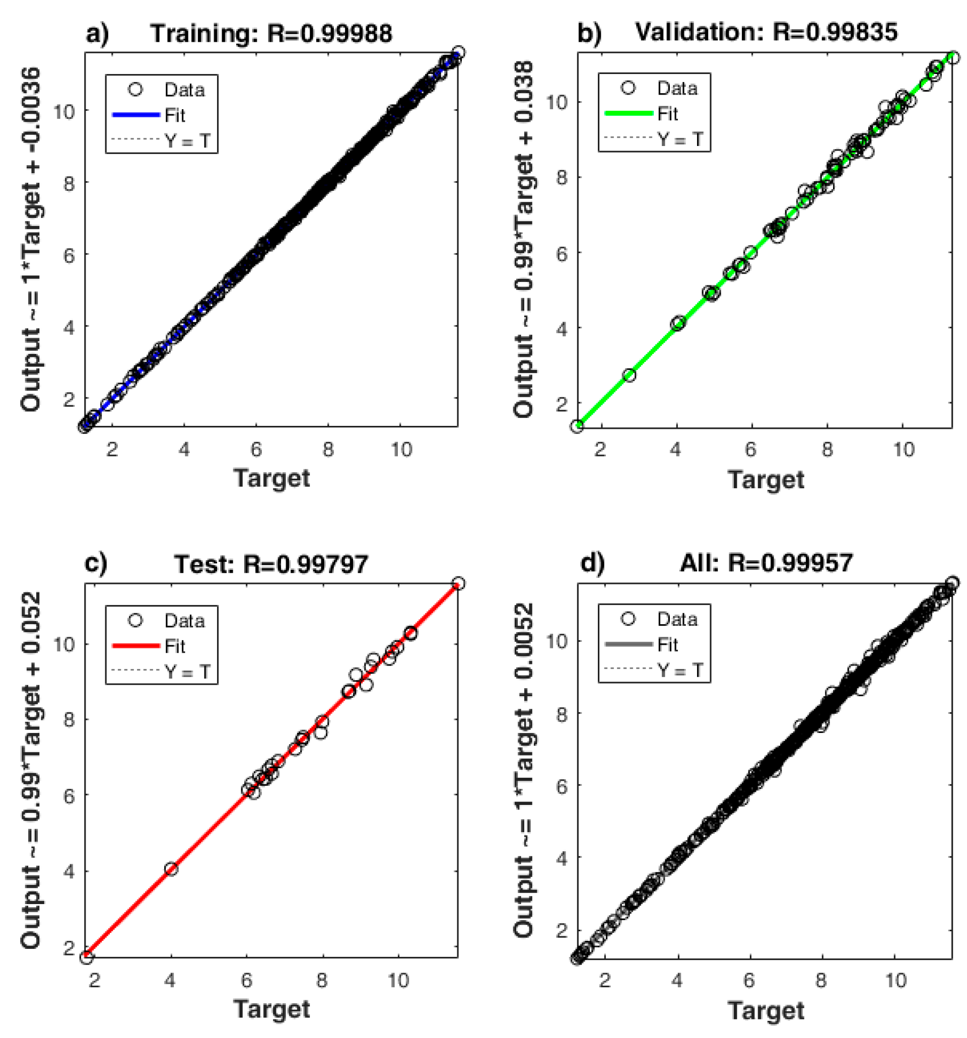
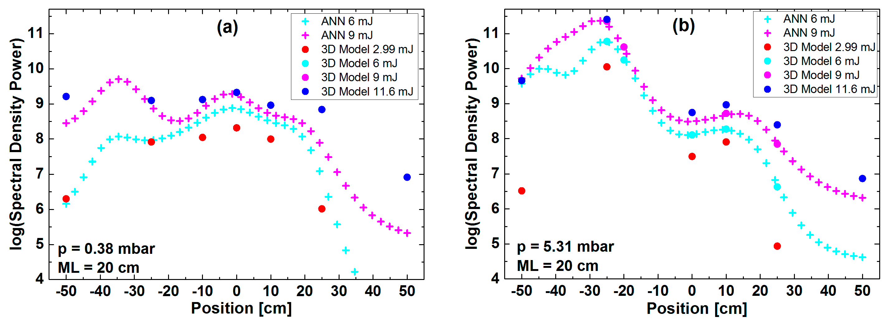
3.1. Testing the ANN against the Full 3D Simulation Results

The optimum topology of the ANN is found to have 11 neurons in the first hidden layer and 17 neurons in the second hidden layer. To obtain this topology several ANNs are trained and for each the number of neurons in the hidden layers is being found by systematically testing the ANN performance. The best ANN is chosen such that the model has the highest correlation factor and the lowest relative errors. In this respect, for this best trained ANN the Pearson coefficient and mean relative errors are calculated for the training and validation data subsets and its prediction capabilities are tested considering a subset of data that were not yet seen by the model (i.e., the testing data subset). The excellent correlation between the experimental results (from 3D simulations) and the predicted values is demonstrated by the regression plots and the high Pearson coefficients (Figure 4).
From Figure 4 one can observe that the correlation factor has values greater than 0.99 for all data subsets: 0.9998 for the training data subset, 0.9983 for the validation data subset, 0.9979 for the testing data and 0.9996 for the overall data set. As a consequence, the best linear fit of the points and the dotted line that represents the perfect correlation (R = 1) overlap, indicating an extremely reduced deviance of the ANN predictions from the 3D model data. The high performance of the ANN is also demonstrated by the low relative errors which are calculated for the three data sets and are presented in Table 1.
The maximum value of the relative error is 4.48% and is obtained for the validation data subset. The testing data subset has a similar maximum relative error of 3.94%, whereas the training data subset has a value of 1.8%. In case of the mean relative errors, the testing data subset has the highest relative errors among the three data subsets, with a fairly reduced value of 1.41%. This is expected, as the input testing subset of data was processed by the ANN only after the training-validation step, in order to prove its prediction capacity for the newly met testing data.
As a result of the excellent ANN prediction capabilities (extremely low relative errors and high correlation factors), the model was further used to predict the harmonic yield for various input variables. In further applications it is very important to have sufficient flux in a given spectral domain, therefore increasing the harmonic yield is of great interest.
We here show that the correctly trained ANN predicts the expected harmonic yield of a possible HHG experiment with the parameters changing in the given range. The ANN works best if the new parameters take values in the range of those used for training and validation. At first glance it may look as a typical interpolation in the multivariable space, however if we consider the complexity of the HHG process given by the highly nonlinear nature of the laser-atom interaction, entangled in the macroscopic effects like propagation, phase matching, etc., then we can understand that the potential of a good prediction method goes far beyond the capabilities of an interpolation.

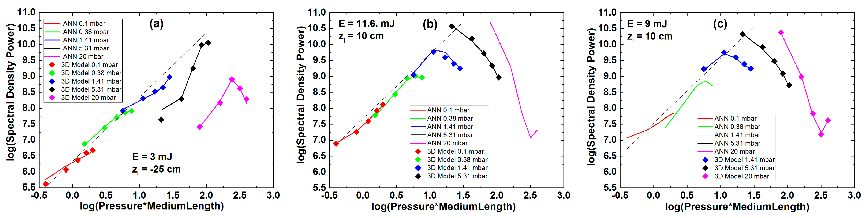
3.2. Prediction Potential of the ANN

The quantity we propose to predict as the main outcome of a virtual HHG experiment is the logarithm of the harmonic yield (Equation (1)) in the specified spectral domain, namely in the 20–40 eV region (between harmonic orders H13–H27). We have chosen this quantity because it can be directly related to the total photon flux in the specified spectral domain which is of central interest in any attosecond science experiment. Since the harmonic yield spans several orders of magnitude, it was more convenient in the training procedure to take its logarithm as the output quantity.
One very important parameter in a HHG experiment is the optical density of the generation medium. In the usual cases the length of the interaction medium is constant, thus the optical density is proportional to the gas pressure. However, since we have as scanning parameter the medium length as well, we here use p × Lmed as parameter, a quantity which is proportional to the optical density. In the absorption limited HHG regime the harmonic yield (i.e., the total photon number) should grow with the square of the optical density in a configuration with fixed phase-matching conditions [64]. In order to have better insight into the physics of how the harmonic yield evolves with the optical density of the medium, we show the results as a function of the log10(p[mbar] × Lmed[cm]).
In Figure 5 we show the prediction capability of the ANN. Dots represent full 3D calculations, while the “+” symbols are the ANN predicted yields for two intermediate pulse energies, namely 6 mJ and 9 mJ. In Figure 5 we represent the expected evolution of the harmonic yield as a function of the gas cell position relative to focus for different laser pulse energy values, while the gas pressure and medium length are fixed: (a) p = 0.38 mbar and Lmed = 20 cm; (b) p = 5.31 mbar and Lmed = 20 cm. Comparing the data in (a) and (b), we expect that the ratio of the yields for the same pulse energy should be close to the ratio of the square of the pressures (around 200) which is clearly not the case. This is because the cell position is a critical factor in every HHG process, influencing the yield via propagation of the fields, phase-matching effects and absorption of the harmonics.
The prediction potential of the ANN simulation proves to be excellent, and captures the highly nonlinear dependence of the macroscopic harmonic yield on many parameters. Especially important conclusion can be drawn from the position-dependence of the yield, namely that very high input pulse energy is not in all cases necessary in order to obtain high harmonic efficiency. Harmonic yield predicted with E = 9 mJ pulse is almost as high as those obtained from 3D simulations with E = 11.6 mJ pulse energy. In order to correctly interpret the results we compare the full 3D simulation results with the ANN predictions as presented in Figure 5b. Magenta dots are yields from 3D simulations and agree well with magenta “+” symbols which are yields predicted by the ANN, being a signature of the ANN high performance. Blue dots are yields obtained from 3D simulations with 11.6 mJ pulse energy. At the zi = −25 cm starting position the ANN predicts the same high yield also for 9 mJ input energy. Even if we use logarithmic scale, the yields predicted with 9 mJ are very close to those obtained with 11.6 mJ. The explanation for this situation can be found in the self-guiding propagation of strong laser pulses in ionizing medium. This result can be good news for attosecond science infrastructures where the other parameters—including cell position and length—are tunable, but the available laser power is limited.
Particularly, the ANN simulation was able to reproduce the transition between two different regimes of laser pulse propagation and consequently different conditions for HHG. At low pulse energy (i.e., starting intensity) and also low pressure conditions we find two comparable maxima of conversion efficiency—see data in Figure 5a with the cell positions before and after the focus. The harmonic yield is calculated with Equation (1), where the radial integration guaranties that off-axis contributions are also taken into account. In these mild macroscopic conditions the fundamental pulse does not suffer serious distortions during propagation, therefore we find a confirmation of the phase-matching model of Balcou [65,66]: in the converging beam harmonics find favorable phase-matching conditions off-axis; while in the diverging beam collinear phase-matching on-axis helps the constructive build-up of the generated harmonic field. The situation is different at higher pressure as seen in Figure 5b. The maximum conversion efficiency found in the whole explored multi-dimensional parameter space has been found at E = 11.6 mJ, p = 5.31 mbar, zi = −25 cm, Lmed = 16 cm. The maximum harmonic yield in Figure 5b (p = 5.31 mbar) is two orders of magnitude higher than the maximum yield in Figure 5a (p = 0.38 mbar). The physical reason for this behavior is that the conditions for the formation of a self-guided beam propagation are fulfilled. A stable “working intensity” is maintained in a large interaction volume (both axially and radially) which creates good phase-matching conditions for a range of harmonics. The conditions that have to be fulfilled in order to have plasma-core induced self-guiding, as well as its effect on the phase-matching of HHG was also studied [67], but goes beyond the scope of this paper.
The ANN has no knowledge about the physics of HHG, however it has been trained with data that contain synthetically the whole nonlinear process. It is highly recommended to perform the complete 3D simulation in cases when ANN predicts less intuitive output. In Figure 6 we present the main results obtained with the full 3D model for the parameter combination (9 mJ; 5.31 mbar; −25 cm; 20 cm). The power spectrum in Figure 6a confirms that the highest yield is expected towards the end of the interaction region. In Figure 6b we show the spatial (r,z) evolution of the laser pulse’s peak intensity, which confirms the formation of a self-guided propagation regime with stable peak intensity 2.5–3 × 10¹⁴ W/cm2. Figure 6c shows the spatial (r,z) evolution of the harmonic order H25. In accordance with the power spectrum, it is confirmed that H25 builds up constructively and attains maximum yield towards the end of the interaction region, predominantly off-axis. In correlation with the evolution of the fundamental pulse (Figure 6b) the spatial region of maximum H25 intensity is the same where the off-axis refocalization of the fundamental beam happens.
In the absorption limited HHG regime the harmonic yield (i.e., the output photon number) should grow quadratically with the optical density under given phase-matching conditions [64]. In Figure 7 we represent the harmonic yield as function of the optical density of the medium. Symbols are data coming from the full 3D simulations, lines are the results predicted by the ANN. With dashed line we show as guide to the eye the line with slope = 2. In Figure 7a,b the 3D simulations provide sufficient data and they confirm that under low optical density conditions the quadratic growth of the yield is valid. Data in Figure 7c have been obtained for an intermediate pulse energy E = 9 mJ and the cell positioned in the diverging beam at zi = 10 cm. In this parameter combination there are few 3D simulation results available, being a good opportunity to test the accuracy of the ANN against the basic physics of the HHG process. Figure 7c shows that the ANN works correctly in this respect, predicting quadratic growth of the yield in the low density regime. Moreover, the end of the region for the absorption limited HHG is also reproduced in a similar manner by the ANN as by the complete 3D simulations. It is not possible to show all results, but the main conclusion is that the ANN is capable to predict regions in the multi-dimensional parameter space where the absorption limited HHG can take place. Furthermore, ANN also predicts for which parameter combinations there is a transition from the initially absorption limited HHG to a saturation, then to a drop in obtainable harmonic yield. This dynamics is represented for example in Figure 7b,c at pressure values 0.38 mbar (green symbols and lines) and 1.41 mbar (blue symbols and lines).

4. Conclusions

In this work, we presented preliminary results for the prediction of the harmonic yield in different HHG configurations. The results have been obtained with the combination of a complete 3D simulation model and an artificial neural network model. The main result of this work is that we succeeded to build a complex computational tool which is able to predict the expected outcome of a HHG experiment covering conditions when several experimental parameters are varied in a given range. Since this is a usual situation in most attosecond science laboratories, we consider our achievement being a useful and very practical numerical instrument. We need to perform a sufficient number of full 3D simulations designed such as to cover (if possible uniformly) the whole explored parameter space. The next step is to introduce these results as input into the ANN, train it, validate and test. A correctly trained ANN is capable to predict the expected outcome of a possible HHG experiment to be performed with parameter combinations that were not implemented in the 3D simulations.
In general terms: the 3D model for HHG combined with the ANN model provide a smooth scan of the parameter space along any variable parameter, and can indicate combinations of possible experimental circumstances which are favorable for the targeted outcome.
In particular: within the present study we targeted to obtain enhanced harmonic yield in the 20–40 eV spectral domain. The variable experimental parameters were: input laser pulse energy E = [0.77; 11.6] mJ; argon pressure p = [0.1; 20] mbar; cell entrance position relative to the nominal focus zi = [−50; 50] cm, medium length Lmed = [0; 20] cm, while we kept unchanged the pulse duration, wavelength, focal length, beam size, gas type.
The main message of the obtained results is that a correctly trained ANN fed with reliable input data originating from the full 3D calculations is capable to predict the outcome of a HHG experiment in the unexplored parts of the multi-dimensional parameter space.
In this particular case study we only demonstrated the capabilities of the prediction method which uses the results of full 3D simulations as input and the harmonic yield as output. However, other physical quantities of interest can be defined and predicted if the ANN is modified accordingly. We can define for example a spectral domain where we search for the existence of isolated attosecond pulse; if it has satellites, then we can predict the contrast relative to the main pulse; we can look for the configuration which provides highest brightness for a specified harmonic order, i.e., high yield combined with low divergence.
ANN as a numerical instrument for prediction can use as input data either data originating from complex simulations (like in our case), or real experimental data (if available), or even a combination of experimental and simulation results. Obviously in the latter case one has to check for the agreement between them, and to perform a calibration of the simulated against the experimental data.
We foresee that this prediction method can be extended to become an easy to use optimization tool, which would mean an essential progress in the way to solve the problem of low conversion efficiency in HHG.

Author Contributions

Conceptualization, V.T.; Software, V.T. (3D model), M.V.C. (ANN model); Validation, K.K. and A.M.M.G.; Investigation, K.K. and A.M.M.G.; Running and analysis of the 3D simulations, K.K.; Running and analysis of the ANN simulations, A.M.M.G.; Writing-Original Draft Preparation, K.K. and A.M.M.G.; Writing-Review & Editing, K.K., A.M.M.G. and V.T.; Visualization, K.K. and A.M.M.G.; All authors discussed the results and contributed to the final manuscript. K.K. and A.M.M.G. contributed equally to this work.

Funding

This research was funded by the Romanian Ministry of Research and Innovation (MCI) Core Program project no. PN 18 03 02/01.

Acknowledgments

We acknowledge the Data Center of INCDTIM Cluj-Napoca where the 3D simulations have been performed.

Conflicts of Interest

The authors declare no conflict of interest.

References

  1. Krausz, F.; Ivanov, M. Attosecond physics. Rev. Modern Phys. 2009, 81, 163–234. [Google Scholar] [CrossRef]
  2. Calegari, F.; Sansone, G.; Stagira, S.; Vozzi, C.; Nisoli, M. Advances in attosecond science. J. Phys. B At. Mol. Opt. Phys. 2016, 49, 062001. [Google Scholar] [CrossRef] [Green Version]
  3. Tate, J.; Auguste, T.; Muller, H.G.; Salières, P.; Agostini, P.; Dimauro, L.F. Scaling of wave-packet dynamics in an intense midinfrared Field. Phys. Rev. Lett. 2007, 98, 1–4. [Google Scholar] [CrossRef] [PubMed]
  4. Kühn, S.; Dumergue, M.; Kahaly, S.; Mondal, S.; Füle, M.; Csizmadia, T.; Farkas, B.; Major, B.; Várallyay, Z.; Calegari, F.; et al. The ELI-ALPS facility: The next generation of attosecond sources. J. Phys. B At. Mol. Opt. Phys. 2017, 50, 132002. [Google Scholar] [CrossRef]
  5. Heyl, C.M.; Güdde, J.; Lhuillier, A.; Höfer, U. High-order harmonic generation with μJ laser pulses at high repetition rates. J. Phys. B At. Mol. Opt. Phys. 2012, 45, 074020. [Google Scholar] [CrossRef]
  6. Rudawski, P.; Heyl, C.M.; Brizuela, F.; Schwenke, J.; Persson, A.; Mansten, A.; Rakowski, R.; Rading, L.; Campi, F.; Kim, B.; et al. A high-flux high-order harmonic source. Rev. Sci. Instrum. 2013, 84, 073103. [Google Scholar] [CrossRef] [PubMed] [Green Version]
  7. Gibson, E.A.; Paul, A.; Wagner, N.; Tobey, R.; Gaudiosi, D.; Backus, S.; Christov, I.P.; Aquila, A.; Gullikson, E.M.; Attwood, D.T.; et al. Coherent Soft X-ray Generation in the Water Window with Quasi—Phase Matching. Science 2003, 302, 95–98. [Google Scholar] [CrossRef] [PubMed]
  8. Sidorenko, P.; Kozlov, M.; Bahabad, A.; Popmintchev, T.; Murnane, M.; Kapteyn, H.; Cohen, O. Sawtooth grating-assisted phase-matching. Opt. Express 2010, 18, 22686–22692. [Google Scholar] [CrossRef] [PubMed]
  9. Serrat, C.; Biegert, J. All-regions tunable high harmonic enhancement by a periodic static electric field. Phys. Rev. Lett. 2010, 104, 1–4. [Google Scholar] [CrossRef] [PubMed]
  10. Biegert, J.; Austin, D.R. Attosecond pulse shaping using partial phase matching. New J. Phys. 2014, 16, 113011. [Google Scholar] [CrossRef] [Green Version]
  11. O’Keeffe, K.; Lloyd, D.T.; Hooker, S.M. Quasi-phase-matched high-order harmonic generation using tunable pulse trains. Opt. Express 2014, 22, 7722–7732. [Google Scholar] [CrossRef] [PubMed]
  12. Ganeev, R.A.; Suzuki, M.; Kuroda, H. Quasi-phase-matching of high-order harmonics in multiple plasma jets. Phys. Rev. A At. Mol. Opt. Phys. 2014, 89, 2–7. [Google Scholar] [CrossRef]
  13. Ganeev, R.A.; Toşa, V.; Kovács, K.; Suzuki, M.; Yoneya, S.; Kuroda, H. Influence of ablated and tunneled electrons on quasi-phase-matched high-order-harmonic generation in laser-produced plasma. Phys. Rev. A At. Mol. Opt. Phys. 2015, 91, 1–8. [Google Scholar] [CrossRef]
  14. Strelkov, V.V.; Ganeev, R.A. Quasi-phase-matching of high-order harmonics in plasma plumes: Theory and experiment. Opt. Express 2017, 25, 21068–21083. [Google Scholar] [CrossRef] [PubMed]
  15. Cormier, E.; Lewenstein, M. Optimizing the effciency in high order harmonic generation optimization by two-color fields. Eur. Phys. J. D 2000, 12, 227. [Google Scholar] [CrossRef]
  16. Schütte, B.; Weber, P.; Kovács, K.; Balogh, E.; Major, B.; Tosa, V.; Han, S.; Vrakking, M.J.J.; Varjú, K.; Rouzée, A. Bright attosecond soft X-ray pulse trains by transient phase-matching in two-color high-order harmonic generation. Opt. Express 2015, 23, 33947. [Google Scholar] [CrossRef] [PubMed] [Green Version]
  17. Luo, J.; Hong, W.; Zhang, Q.; Liu, K.; Lu, P. Dramatic cutoff extension and broadband supercontinuum generation in multi-cycle two color pulses. Opt. Express 2012, 20, 9801. [Google Scholar] [CrossRef] [PubMed]
  18. Chipperfield, L.E.; Robinson, J.S.; Tisch, J.W.G.; Marangos, J.P. Ideal waveform to generate the maximum possible electron recollision energy for any given oscillation period. Phys. Rev. Lett. 2009, 102, 2–5. [Google Scholar] [CrossRef] [PubMed]
  19. Haessler, S.; Balčiunas, T.; Fan, G.; Andriukaitis, G.; Pugžlys, A.; Baltuška, A.; Witting, T.; Squibb, R.; Zaïr, A.; Tisch, J.W.G.; et al. Optimization of Quantum Trajectories Driven by Strong-Field Waveforms. Phys. Rev. X 2014, 4, 021028. [Google Scholar] [CrossRef]
  20. Winterfeldt, C.; Spielmann, C.; Gerber, G. Colloquium: Optimal control of high-harmonic generation. Rev. Modern Phys. 2008, 80, 117–140. [Google Scholar] [CrossRef]
  21. Jin, C.; Wang, G.; Le, A.-T.; Lin, C.D. Route to optimal generation of soft X-ray high harmonics with synthesized two-color laser pulses. Sci. Rep. 2014, 4, 7067. [Google Scholar] [CrossRef] [PubMed] [Green Version]
  22. Balogh, E.; Bódi, B.; Tosa, V.; Goulielmakis, E.; Varjú, K.; Dombi, P. Genetic optimization of attosecond-pulse generation in light-field synthesizers. Phys. Rev. A At. Mol. Opt. Phys. 2014, 90, 1–7. [Google Scholar] [CrossRef]
  23. Bódi, B.; Balogh, E.; Tosa, V.; Goulielmakis, E.; Varjú, K.; Dombi, P. Attosecond pulse generation with an optimization loop in a light-field-synthesizer. Opt. Express 2016, 24, 21957. [Google Scholar] [CrossRef] [PubMed]
  24. Xi, J.; Xue, Y.; Xu, Y.; Shen, Y. Artificial neural network modeling and optimization of ultrahigh pressure extraction of green tea polyphenols. Food Chem. 2013, 141, 320–326. [Google Scholar] [CrossRef] [PubMed]
  25. Neocleous, C.; Schizas, C. Artificial Neural Network Learning: A Comparative Review. In Methods and Applications of Artificial Intelligence; Lecture Notes in Computer Science; Springer: Berlin/Heidelberg, Germany, 2002; Volume 2308, pp. 300–313. [Google Scholar]
  26. Maleki, N.; Kashanian, S.; Maleki, E.; Nazari, M. A novel enzyme based biosensor for catechol detection in water samples using artificial neural network. Biochem. Eng. J. 2017, 128, 1–11. [Google Scholar] [CrossRef]
  27. Belalia Douma, O.; Boukhatem, B.; Ghrici, M.; Tagnit-Hamou, A. Prediction of properties of self-compacting concrete containing fly ash using artificial neural network. Neural Comput. Appl. 2017, 28, 707–718. [Google Scholar] [CrossRef]
  28. Sitton, J.D.; Zeinali, Y.; Story, B.A. Rapid soil classification using artificial neural networks for use in constructing compressed earth blocks. Constr. Build. Mater. 2017, 138, 214–221. [Google Scholar] [CrossRef]
  29. Cimpoiu, C.; Cristea, V.M.; Hosu, A.; Sandru, M.; Seserman, L. Antioxidant activity prediction and classification of some teas using artificial neural networks. Food Chem. 2011, 127, 1323–1328. [Google Scholar] [CrossRef] [PubMed]
  30. Durodola, J.F.; Li, N.; Ramachandra, S.; Thite, A.N. A pattern recognition artificial neural network method for random fatigue loading life prediction. Int. J. Fatigue 2017, 99, 55–67. [Google Scholar] [CrossRef]
  31. Cristea, M.V.; Roman, R.; Agachi, S.P. Neural Networks Based Model Predictive Control of the Drying Process. Eur. Symp. Comput. Aided Process Eng. 2003, 13, 389–394. [Google Scholar]
  32. Bouhoune, K.; Yazid, K.; Boucherit, M.S.; Chériti, A. Hybrid control of the three phase induction machine using artificial neural networks and fuzzy logic. Appl. Soft Comput. J. 2017, 55, 289–301. [Google Scholar] [CrossRef]
  33. Mihet, M.; Cristea, V.M.; Agachi, S.P. FCCU simulation based on first principle and artificial neural network models. Asia-Pac. J. Chem. Eng. 1999, 4, 878–884. [Google Scholar] [CrossRef]
  34. Erzin, Y.; Ecemis, N. The use of neural networks for the prediction of cone penetration resistance of silty sands. Neural Comput. Appl. 2017, 28, 727–736. [Google Scholar] [CrossRef]
  35. Bhatikar, S.R.; DeGroff, C.; Mahajan, R.L. A classifier based on the artificial neural network approach for cardiologic auscultation in pediatrics. Artif. Intell. Med. 2005, 33, 251–260. [Google Scholar] [CrossRef] [PubMed]
  36. Hakeem, M.A.; Kamil, M. Analysis of artificial neural network in prediction of circulation rate for a natural circulation vertical thermosiphon reboiler. Appl. Therm. Eng. 2017, 112, 1057–1069. [Google Scholar] [CrossRef]
  37. Chen, Z.; Ma, W.; Wei, K.; Wu, J.; Li, S.; Xie, K.; Lv, G. Artificial neural network modeling for evaluating the power consumption of silicon production in submerged arc furnaces. Appl. Therm. Eng. 2017, 112, 226–236. [Google Scholar] [CrossRef]
  38. Oladunjoye, A.O.; Oyewole, S.A.; Singh, S.; Ijabadeniyi, O.A. Prediction of Listeria monocytogenes ATCC 7644 growth on fresh-cut produce treated with bacteriophage and sucrose monolaurate by using artificial neural network. LWT Food Sci. Technol. 2017, 76, 9–17. [Google Scholar] [CrossRef]
  39. Youshia, J.; Ali, M.E.; Lamprecht, A. Artificial neural network based particle size prediction of polymeric nanoparticles. Eur. J. Pharm. Biopharm. 2017, 119, 333–342. [Google Scholar] [CrossRef] [PubMed]
  40. Gherman, A.M.M.; Tosa, N.; Cristea, M.V.; Tosa, V.; Porav, S. Artificial neural networks modeling of the parameterized gold nanoparticles generation through photo-induced process. Mater. Res. Express 2018, 5. [Google Scholar] [CrossRef]
  41. Lagaris, I.E.; Likas, A.; Fotiadis, D.I. Artificial neural network methods in quantum mechanics. Comput. Phys. Commun. 1997, 104, 1–14. [Google Scholar] [CrossRef] [Green Version]
  42. Kim, H.T.; Kim, I.J.; Tosa, V.; Lee, Y.S.; Nam, C.H. High brightness harmonic generation at 13 nm using self-guided and chirped femtosecond laser pulses. Appl. Phys. B Lasers Opt. 2004, 78, 863–867. [Google Scholar] [CrossRef]
  43. Kovács, K.; Major, B.; Kőrös, C.P.; Rudawski, P.; Heyl, C.M.; Johnsson, P.; Arnold, C.L.; L’Huillier, A.; Toşa, V.; Varjú, K. Multi-parameter optimization of a loose focusing high flux high-harmonic beamline. J. Phys. B At. Mol. Opt. Phys. 2018, submitted. [Google Scholar]
  44. Tosa, V.; Takahashi, E.; Nabekawa, Y.; Midorikawa, K. Generation of high-order harmonics in a self-guided beam. Phys. Rev. A 2003, 67, 063817. [Google Scholar] [CrossRef]
  45. Priori, E.; Cerullo, G.; Nisoli, M.; Stagira, S.; De Silvestri, S.; Villoresi, P.; Poletto, L.; Ceccherini, P.; Altucci, C.; Bruzzese, R.; et al. Nonadiabatic three-dimensional model of high-order harmonic generation in the few-optical-cycle regime. Phys. Rev. A 2000, 61, 1–8. [Google Scholar] [CrossRef]
  46. Lewenstein, M.; Balcou, P.; Ivanov, M.Y.; L’Huillier, A.; Corkum, P.B. Theory of high-harmonic generation by low-frequency laser fields. Phys. Rev. A 1994, 49, 2117–2132. [Google Scholar] [CrossRef] [PubMed]
  47. Tosa, V.; Kovacs, K.; Altucci, C.; Velotta, R. Generating single attosecond pulse using multi-cycle lasers in a polarization gate. Opt. Express 2009, 17, 17700–17710. [Google Scholar] [CrossRef] [PubMed]
  48. Balogh, E.; Kovacs, K.; Dombi, P.; Fulop, J.A.; Farkas, G.; Hebling, J.; Tosa, V.; Varju, K. Single attosecond pulse from terahertz-assisted high-order harmonic generation. Phys. Rev. A At. Mol. Opt. Phys. 2011, 84, 1–9. [Google Scholar] [CrossRef]
  49. Negro, M.; Vozzi, C.; Kovacs, K.; Altucci, C.; Velotta, R.; Frassetto, F.; Poletto, L.; Villoresi, P.; de Silvestri, S.; Tosa, V.; et al. Gating of high-order harmonics generated by incommensurate two-color mid-IR laser pulses. Laser Phys. Lett. 2011, 8, 875–879. [Google Scholar] [CrossRef]
  50. Tosa, V.; Altucci, C.; Kovcs, K.; Negro, M.; Stagira, S.; Vozzi, C.; Velotta, R. Isolated attosecond pulse generation by two-mid-ir laser fields. IEEE J. Sel. Top. Quantum Electron. 2012, 18, 239–247. [Google Scholar] [CrossRef]
  51. Balogh, E.; Kovács, K.; Toşa, V.; Varjú, K. A case study for terahertz-assisted single attosecond pulse generation. J. Phys. B At. Mol. Opt. Phys. 2012, 45, 074022. [Google Scholar] [CrossRef] [Green Version]
  52. Kovacs, K.; Tosa, V.; Major, B.; Balogh, E.; Varju, K. High-Efficiency Single Attosecond Pulse Generation with a Long-Wavelength Pulse Assisted by a Weak Near-Infrared Pulse. IEEE J. Sel. Top. Quantum Electron. 2015, 21. [Google Scholar] [CrossRef]
  53. Major, B.; Balogh, E.; Kovács, K.; Han, S.; Schütte, B.; Weber, P.; Vrakking, M.J.J.; Tosa, V.; Rouzée, A.; Varjú, K. Spectral shifts and asymmetries in mid-infrared assisted high-order harmonic generation. J. Opt. Soc. Am. B 2018, 35, A32. [Google Scholar] [CrossRef]
  54. Tosa, V.; Kovács, K.; Ursescu, D.; Varjú, K. Characteristics of femtosecond laser pulses propagating in multiply ionized rare gases. Nuclear Instrum. Methods Phys. Res. B 2017, 408, 271–275. [Google Scholar] [CrossRef]
  55. Tosa, V.; Kovács, K.; Major, B.; Balogh, E.; Varjú, K. Propagation effects in highly ionised gas media. Quantum Electron. 2016, 46, 321–326. [Google Scholar] [CrossRef] [Green Version]
  56. Nabipour, M. Prediction of surface tension of binary refrigerant mixtures using artificial neural networks. Fluid Phase Equilib. 2018, 456, 151–160. [Google Scholar] [CrossRef]
  57. Cristea, M.V.; Varvara, S.; Muresan, L.; Popescu, I.C. Neural networks approach for simulation of electrochemical impedance diagrams. Indian J. Chem. 2002, 42, 764–768. [Google Scholar]
  58. Rezakazemi, M.; Razavi, S.; Mohammadi, T.; Nazari, A.G. Simulation and determination of optimum conditions of pervaporative dehydration of isopropanol process using synthesized PVA-APTEOS/TEOS nanocomposite membranes by means of expert systems. J. Membr. Sci. 2011, 379, 224–232. [Google Scholar] [CrossRef]
  59. Vanneschi, L.; Castelli, M. Delta Rule and Backpropagation. Encycl. Bioinform. Comput. Biol. 2019, 621–633. [Google Scholar] [CrossRef]
  60. Hecht-Nielsen, R. Theory of the Backpropagation Neural Network. In Proceedings of the International 1989 Joint Conference on Neural Networks, Washington, DC, USA, 18–22 June 1989; Volume 1, pp. 593–605. [Google Scholar] [CrossRef]
  61. Hyperbolic Tangent Sigmoid Transfer Funcion. Available online: https://www.mathworks.com/help/deeplearning/ref/tansig.html;jsessionid=5a52bc6806308ec1f28edf572e5d (accessed on 30 October 2018).
  62. Hagan, M.T.; Menhaj, M.B. Training Feedforward Networks with the Marquardt Algorithm. IEEE Trans. Neural Netw. 1994, 5, 989–993. [Google Scholar] [CrossRef] [PubMed]
  63. Hagan, M.T.; Demuth, H.B.; Beale, M.H.; De Jesús, O. Neural Network Design, 2nd ed. eBook. 2014. Available online: hagan.okstate.edu/nnd.html (accessed on 30 October 2018).
  64. Constant, E.; Garzella, D.; Breger, P.; Mével, E.; Dorrer, C.; Le Blanc, C.; Salin, F.; Agostini, P. Optimizing High Harmonic Generation in Absorbing Gases: Model and Experiment. Phys. Rev. Lett. 1999, 82, 1668–1671. [Google Scholar] [CrossRef]
  65. Balcou, P.; Salieres, P.; L’Huillier, A.; Lewenstein, M. Generalized phase-matching conditions for high harmonics: The role of field-gradient forces. Phys. Rev. A 1997, 55, 3204–3210. [Google Scholar] [CrossRef]
  66. Salières, P.; L’Huillier, A.; Lewenstein, M. Coherence control of high-order harmonics. Phys. Rev. Lett. 1995, 74, 3776–3779. [Google Scholar] [CrossRef] [PubMed]
  67. Anderson, D.; Kim, A.V.; Lisak, M.; Mironov, V.A.; Sergeev, A.M.; Stenflo, L. Self-sustained plasma waveguide structures produced by ionizing laser radiation in a dense gas. Phys. Rev. E 1995, 52, 4564–4567. [Google Scholar] [CrossRef]
Figure 1. (a) Flowchart of the computation, (b) Flowchart of the backpropagation algorithm.
Applsci 08 02106 g001
Figure 2. ANN architecture and the schematic representation of a neuron.
Applsci 08 02106 g002
Figure 3. (a) Sketch of the geometrical arrangement: laser pulse propagates from left to right; interaction cell filled with gas at p pressure, begins at zi position relative to focus; Lmed is the length of the interaction medium. (b) Schematic representation of the parameter space where the full 3D calculations have been performed. For each pulse energy full 3D calculations were performed for several cell positions relative to focus (x axis) and gas pressures (y axis). Red bullets represent the particular cases solved by full 3D simulations and used by ANN for training, validation and testing. The forth scanned parameter is the medium length which is included in every simulation with values 4, 8, 12, 16, 20 cm.
Applsci 08 02106 g003
Figure 4. Plot of ANN calculated log10(harmonic yield) against the values obtained with the complete 3D model for the following data subsets: (a) training, (b) validation, (c) testing and (d) overall data.
Applsci 08 02106 g004
Figure 5. Harmonic yield as function of the gas cell position relative to the nominal focus. Dots are data obtained from the complete 3D simulations, “+” symbols are the results of the ANN predictions. Panel (a) synthesizes the results obtained for different laser pulse energies at the fixed parameter values p = 0.38 mbar and Lmed = 20 cm, i.e., at the cell end. Panel (b) shows the results obtained with p = 5.31 mbar and Lmed = 20 cm. Colors of the symbols dots and “+” are the same for the same energy. At the intermediate energies, 6 and 9 mJ, we have performed merely a few but computationally demanding 3D simulations and only with p = 5.31 mbar.
Applsci 08 02106 g005
Figure 6. Results of the complete 3D simulation performed with the following values of the parameters: E = 9 mJ; p = 5.31 mbar; zi = −25 cm. (a) Radially integrated power spectrum calculated at every 4 cm of medium length. (b) (r,z) map of the driving pulse’s intensity spatial evolution. (c) (r,z) map of how the H25 builds up during propagation. Other parameters are specified in the main text at the beginning of Section 3.
Applsci 08 02106 g006
Figure 7. Harmonic yield as function of the optical density of the medium. We represent the logarithm of both quantities, the units are arbitrary. Slope = 2 indicates the quadratic growth of the harmonic yield with the optical density.
Applsci 08 02106 g007
Table 1. The mean and maximum values of the relative error.
|Mean Relative Error| [%]|Maximum Relative Error| [%]
Training Data Subset0.331.80
Validation Data Subset1.044.48
Testing Data Subset1.413.94

