A Novel One-Camera-Five-Mirror Three-Dimensional Imaging Method for Reconstructing the Cavitation Bubble Cluster in a Water Hydraulic Valve

Abstract

In order to study the bubble morphology, a novel experimental and numerical approach was implemented in this research focusing on the analysis of a transparent throttle valve made by Polymethylmethacrylate (PMMA) material. A feature-based algorithm was written using the MATLAB software, allowing the 2D detection and three-dimensional (3D) reconstruction of bubbles: collapsing and clustered ones. The valve core, being an important part of the throttle valve, was exposed to cavitation; hence, to distinguish it from the captured frames, the faster region-based convolutional neural network (R-CNN) algorithm was used to detect its morphology. Additionally, the main approach grouping the above listed techniques was implemented using an optimized virtual stereo vision arrangement of one camera and five plane mirrors. The results obtained during this study validated the robust algorithms and optimization applied.

1. Introduction

Cavitation is an omnipresent phenomenon observed during flows in valves, pipes, pressure vessels, and so on. Its occurrence favors considerable material losses in complex situations, which requires costly replacements to be made thereby causing significant performance drawbacks to industries. Studies on fluid dynamics about solving issues related to cavitation due to bubbles collapse are being done by researchers from both universities and companies. To be more precise, understanding bubble dynamics in valves requires in-depth investigations as the presence of void fractions in optically dense multiphase flows have been hindering the observation of bubbles [1].

To the best of our knowledge, fewer studies about bubble morphology in throttle valves have been done, albeit with both the invasive techniques (impedance probe and optical fiber probe) and the non-invasive techniques (PIV, PTV, PT) being prevalent. The non-invasive approach has widely been promoted through high speed photography in bubble measurement studies, inclusive of the 2D bubble columns [2,3,4,5], the channels [6,7,8,9], the flat plates [10], the hydrofoils [11,12], the mixing tanks [13], the liquid-solid interface [14], the dynamically loaded journal bearings [15], the ultrasonic devices [14,16,17,18], the axisymmetric geometry [10], the throttle orifice, and so on.

To start with, the first ever experiment on capturing the motion of Helium-filled bubbles in an engine using a single camera and multiple mirrors, was done by Kent and Eaton [19] in 1982. Next, Racca and Dawey [20] implemented a measuring method by using a single high speed cine camera through a split field mirror to track small resin beads (tracers) and Belden et al. proposed a “3D synthetic aperture imaging (SA imaging)” by using nine (9) high speed photon cameras to capture the bubbly flow induced by a turbulent circular plunging jet.

Similarly, to study the fluid flow, virtual stereo vision was implemented in this research to observe and reconstruct the 3D bubbles formed in the area between the valve seat, the valve core and the outlet port. Xue et al. [21] applied virtual binocular stereo vision in a glass-made water tank to match and reconstruct the bubble trajectory motion through a “3D polar coordinate homonymy correlation algorithm”, thereby determining the analogous relation of alike bubbles from two-half images. Additional studies by Xue et al. [22,23,24] dealt with the bubble behaviour characteristics in the gas-liquid two-phase flow, modality factors of bubbles, intrinsic and extrinsic parameters of the virtual cameras, and the segmentation of multi-bubbles.

Likewise, by implementing robust algorithms to estimate the velocities and reconstruct the trajectories of bubbles, broad investigations were made by Mitra et al. [25], Acuna et al. [26], Racca et al. [20], Dencks et al. [16], Cheng et al. [27], Krimerman [28], and Bakshi et al. [29], respectively.

For a clearer approach of the stereo vision concept, significant contributions were brought by the following researchers: Feng et al. [30] established a 3D mathematical model to measure a 3D point through a combination of the single camera stereo vision sensor with planar mirror imaging. Upon comparison with the binocular stereo vision, the output in terms of calibration, measurement speed and errors resulted in being more accurate. Figueroa et al. [31] studied a nearly non-dispersed 2D bubbly flow in a thin channel by means of a high speed camera- image processing routine to validate bubble clusters trajectory and sealing arguments to estimate their lifespan. Moreover, bubbly flows were continuously studied by Yucheng et al. [8,32], Chakraborty [33], Lau et al. [3], and Tayler et al. [5] from the last decade. Prolonged observations in dense bubbly flows containing overlapped ellipse-like bubbles through image analysis using algorithms were achieved by de Langlard et al. [34], Honkanen et al. [35,36], and Zhang et al. [37], respectively.

On the other hand, Fujisawa et al. [38] examined erosion caused by bubble implosion and shock waves formed by a cavitating jet. This was carried out using shadowgraph imaging, time-difference analysis, and laser schlieren imaging techniques, thereby giving adequate results.

Similarly, studies about object detection in fluid flow were carried out by Kompella et al. [39] who detected semi-transparent objects in single images, while Hata et al. [40] and Kai et al. [41], emphasized the shape extraction and the dense reconstruction of transparent objects.

On the basis of virtual stereo motion, this paper illustrates a novel approach of using five reflectors (single camera with two-symmetrical reflectors and one stand-alone reflector) in contrast to the literature where single cameras with only two symmetrical reflector sets were used. In addition, compared with using three high-speed cameras, the experimental images reflected from the plane mirrors did not only cut the equipment costs, but also ensured the synchronization of the images from the three directions (x, y, and z). A deep learning method developed by Ren et al. [42] was applied to detect the valve core (opaque) during the bubbly fluid flow. Lastly, the original algorithms written using MATLAB (R2016b, The MathWorks, Inc., Natick, MA, USA) software in this research helped to determine the optimal design of the reflector sets set-up and perform the 3D reconstruction of the bubbles.

The overall structure of the paper is as follows: the introduction is followed by Section 2 in which the overall structure of the 3D imaging experiment system is explained. Next, Section 3 elaborates on the optimized arrangement of the one-camera-five mirror module, while Section 4 illustrates the development of the proposed algorithm used for bubble detection. Finally, Section 5 and Section 6 elucidate on the analysis of the results and the conclusion, respectively.

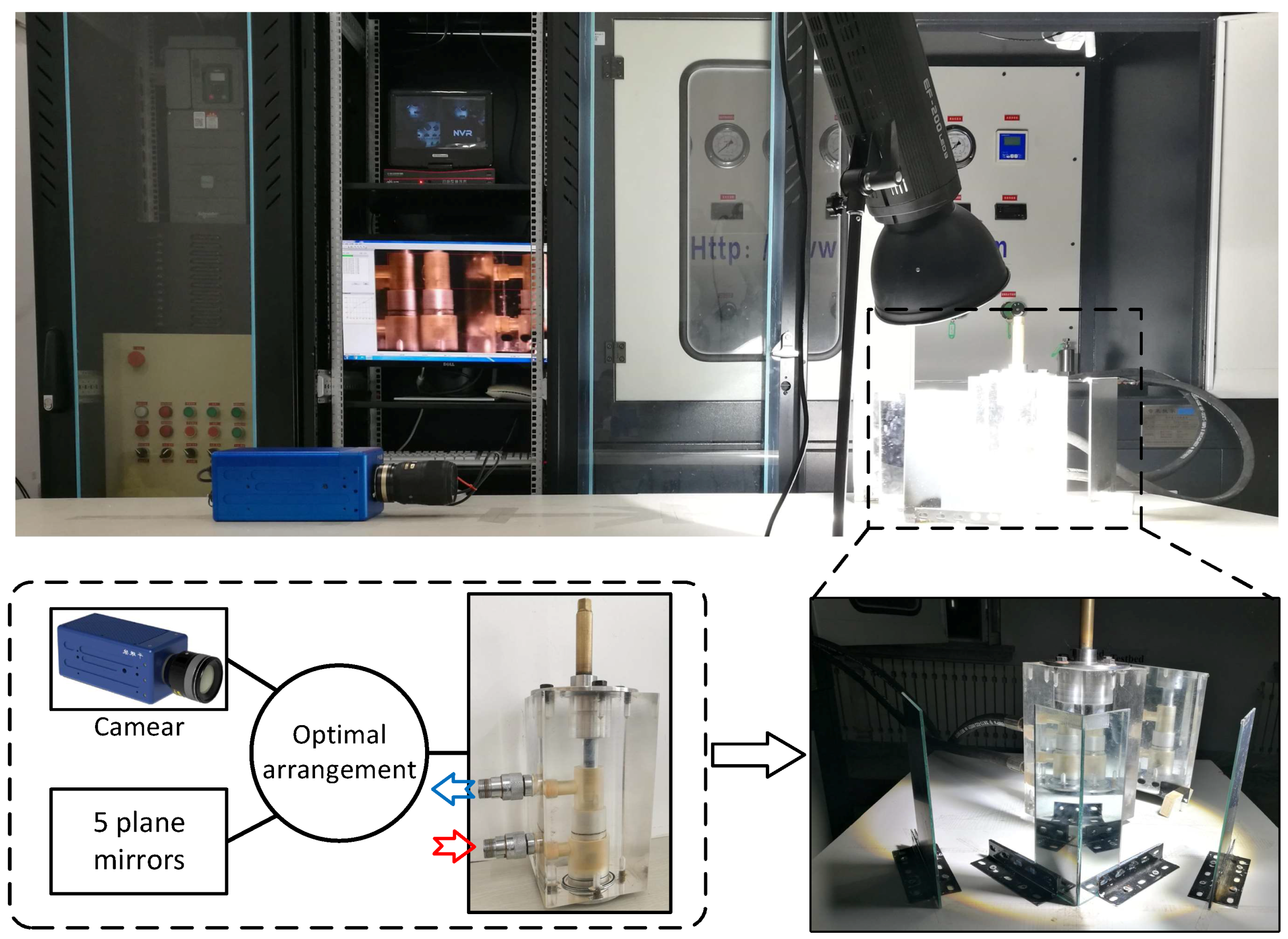
2. Overall Structure of the 3D Imaging Experiment System

Figure 1 shows the experimental setups of the hydraulic system, which consists of a water hydraulic power transmission subsystem, an electric control subsystem and the water hydraulic valve. The dimensions of the transparent valve used in this research were marked in right figure. In addition, the inlet and outlet ports were noted. The “electric control subsystem” consists of a frequency inverter and a component switching panel. The frequency inverter (Schneider Altivar 610, Paris, France) ensures suitable power for the hydraulic test bench through adequate control of the water pumps working frequency (input pressure). Water pump used in the transmission system allows a constant pressure water supply, which eliminates the shortcomings in terms of pressure fluctuations owing to subsequent improvements in the AC frequency conversion technology.

Figure 2 clearly demonstrates the optimal arrangement of the one-camera-five-mirror 3D imaging module on the water hydraulics experiment platform. The arrangement allowed the capture and storing of the experimental videos by the high-speed camera and the computer, respectively. High-speed camera can capture thousands of photographs per second. However, because of the very short time interval of two adjacent pictures, the Light Emitting Diode (LED) lamp was an essential device to compensate for the lack of exposure.

2.1. Measurement Principle of the 3D Imaging

Viewing cavitating bubbles in the fluid flow from one side might not give satisfying results in terms of the size, the position, and the quantity of bubbles. Hence, to avoid partial invisibility while recording, a 3D approach based on one-camera-five-mirror device was applied in this study.

The 3D virtual stereo vision measurement principle of the bubbles illustrated in Figure 3 explains the arrangement of the reflector sets. To observe the cavitating area in a transparent throttle valve through different view angles, a high-speed camera (Revealer 5KF10, Hefei, China) with a 60 mm Nikkor lens (Tokyo, Japan): resolution and frame rate of $1280\times 860$ pixels and 4000 fps, a lighting equipment, and five reflectors (mirror glass) were used. The concept of virtual stereoscopic parallax eased the capturing of the cavitation bubbles around the valve core. With the real camera imaged into virtual cameras: two mirrors positioned symmetrically (L, R) and one mirror placed behind the valve (B). The specular reflection along the inherent optical paths eased mirroring of the real camera. Even with intersecting optical paths, the virtual image planes from the three sides (L, R and B) were distinctively separated on the real camera. Moreover, with the inlet–outlet coupler and the hydraulic hoses hindering the vision, the fourth virtual camera was omitted. As observed during the experiment, this novel method successfully captured clearly both the growth and the collapse of the bubbles.

2.2. Transparent Throttle Valve

In previous studies, the refractive index of glass-made tanks (1.52) [13,21,22,23,24] was suitable for analyzing bubbly flows. However, the advent of an easily machined transparent thermoplastic called Polymethylmethacrylate (PMMA, Perspex, acrylic glass), eased the capturing of images by high speed photography. Along with its refractive index (1.490) being relatively closer to the fluid used (water (1.333)) and its ability to withstand higher pressures of 20 bar, PMMA was used to manufacture the throttle valve’s body. Operating at 20 ${}^{°}$C, no correction factor was required and high light transmission was observed with no substantial image distortion. Having a modular structure, analysis of the bubble features was eased throughout the area under study. To counteract with the effects of high pressure, the chosen material for the valve core was brass while its connecting rod and the valve core were made using stainless steel. In addition, to induce cavitating bubbles in the fluid flow, a pressure difference of 0.2 MPa (the inlet pressure: 0.3 MPa; the outlet pressure: 0.1 MPa) was applied in the valve port area. The bursting effect of the bubbles resulted in the flaking off the materials, thus, eroding the inner area of the valve.

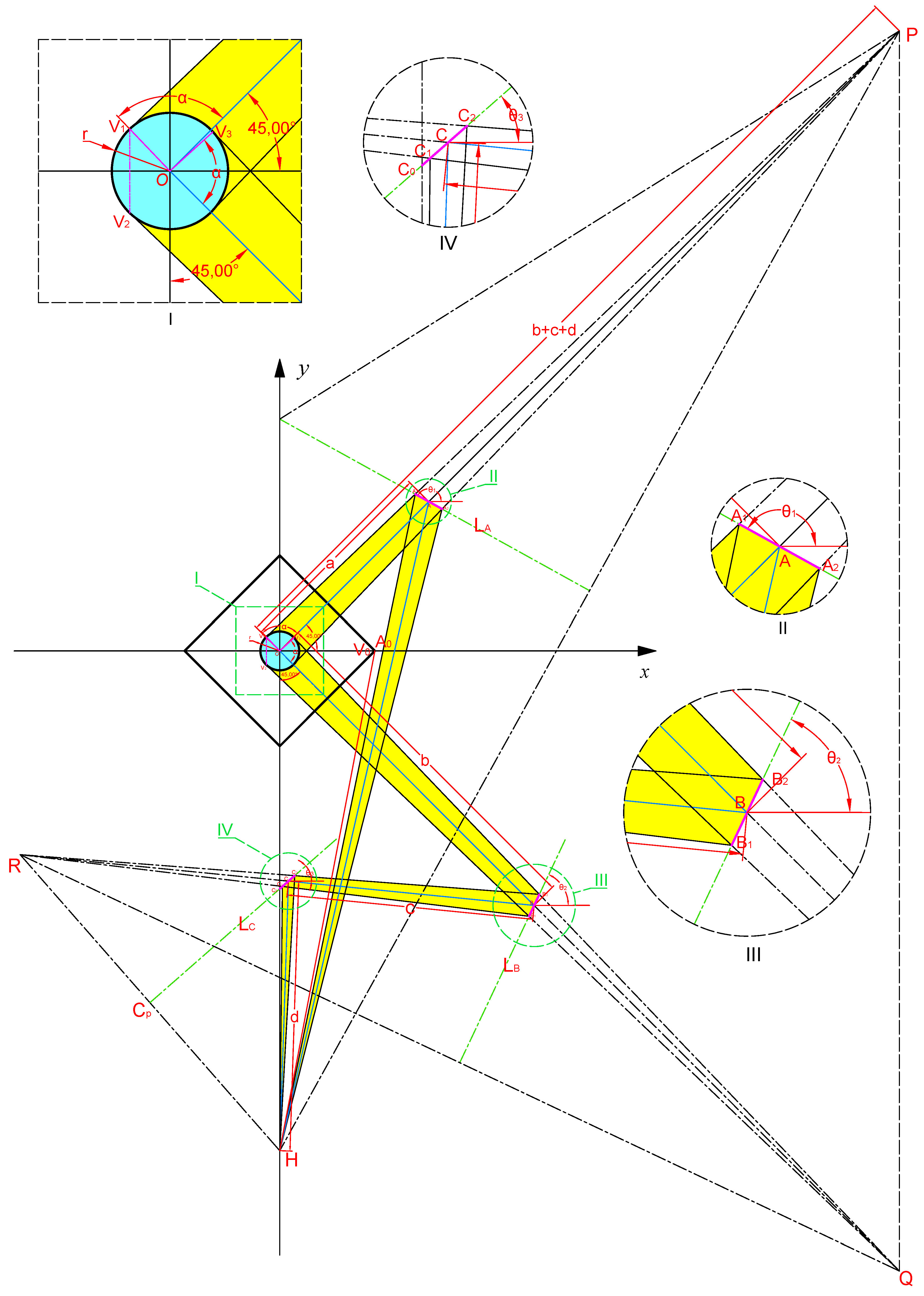
3. Optimization Arrangement of the One-Camera-Five-Mirror Module

The 3D Bubble reconstruction algorithm developed in this paper was based on space rectangular coordinate system. The spatial coordinates of the cavitation bubbles in the valve was provided by the position information of the experiment images from the three directions of left (L), right (R), and back (B). The bubble position coordinates on the horizontal axis from the L and B sides’ images were directly used as the x-coordinate values of the bubbles in the spatial location and the R side’s image provided the y-coordinate values. In case a virtual camera has an oblique angle with the corresponding observed side of the valve, the transparent surface made by PMMA material will cause image refringence, then the 3D bubble position in the x–y plane will be inaccurate with its actual space position. The larger the oblique angle, the greater the error of the bubble in space position. To eliminate this problem, the light center axes of the three virtual cameras were all defined to be perpendicular to the observed faces.

The resolution of the experiment videos was limited by the capability of the high-speed camera and the distance from the observed field to the camera lens. The resolution capability of the camera and the lens used in the experiment are fixed. The cavitation bubbles in the valve were quite small. In order to ensure the resolution of the bubble images, the distance of the optical path were maintained as short as possible. In addition, the distance of the optical path of the three virtual cameras was set to be equal to ensure the consistent image resolution in the L, R and B three sides.

To optimize the arrangement of the high-speed camera and five plane mirrors to meet the expectation above, the optimization model was built. As shown in Figure 4, the point P and Q are the position of the virtual camera 3 (B) and 2 (R) in Figure 3. Due to the symmetrical relationship of the virtual camera 1 (L) and 2 (R), the optimal design of the two mirrors of virtual camera 1 was omitted. Thus, the optimization design variables in practice were the position parameters of the camera (point H) and the three mirrors (marked as A, B and C).

3.1. Optimization Model

As shown in Figure 4, with regard to the nonlinear constrained optimization in this paper, the optimization objective is defined as $J(\mathbf{x})=b+c+d$. The objective function is mathematically defined by:

$$\min J(\mathbf{x}),$$

(1)

Subject to:

$$\left\{\begin{array}{c}\arctan k_{H{C}_2}-\arctan k_{H{V}_0}>\frac{1^{°}}{{180}^{°}}\pi ,\hfill \\ x_{A_0}-x_{V_0}>3,\hfill \\ x_{C_1}>1,\hfill \end{array}\right.$$

where $\mathbf{x}={[a,b,c,d,{\theta }_1,{\theta }_2,{\theta }_3]}^T$.

3.2. Optimization Variables

The four length optimization variables are defined as follows: $l_{OA}=a>0$, $l_{OB}=b>0$, $l_{BC}=c>0$, $l_{CH}=d>0$. The three angle optimization variables are defined as follows ${\theta }_1$ (mirror A), ${\theta }_2$ (mirror B) and ${\theta }_3$ (mirror C). Hence, the optimal objective can be represented as $l_{OP}=l_{OQ}=b+c+d$ and the coordinates of the virtual cameras 2 and 3 are expressed as follows: $Q(\frac{b+c+d}{\sqrt{2}},-\frac{b+c+d}{\sqrt{2}})$, $P(\frac{b+c+d}{\sqrt{2}},\frac{b+c+d}{\sqrt{2}})$. In addition, the coordinates of the plane mirrors A and B can be expressed as $A(\frac{a}{\sqrt{2}},\frac{a}{\sqrt{2}})$, $B(\frac{b}{\sqrt{2}},-\frac{b}{\sqrt{2}})$.

All the coordinates in Figure 4 can be deviated and expressed by the optimization variables, $a,b,c,d,{\theta }_1,{\theta }_2,{\theta }_3$, based on the optical and geometrical relationship among them. In addition, the coordinate values are listed in

Table 1. Coordinate values of the design points.

Point	x coordinate	y coordinate
H	$x_P+y_P\tan {\theta }_1-y_H\tan {\theta }_1$	${\displaystyle \frac{2x_P\tan {\theta }_1+y_P({\tan }^2{\theta }_1-1)+\sqrt{2}a(1-\tan {\theta }_1)}{1+{\tan }^2{\theta }_1}}$
R	$x_Q+y_Q\tan {\theta }_2-y_R\tan {\theta }_2$	${\displaystyle \frac{2x_Q\tan {\theta }_2+y_Q({\tan }^2{\theta }_2-1)-\sqrt{2}b(1+\tan {\theta }_2)}{1+{\tan }^2{\theta }_2}}$
C	${\displaystyle \frac{\frac{y_B-y_R}{x_B-x_R}{x}_R-y_R-\frac{x_R+x_H}{2}\tan {\theta }_3+\frac{y_R+y_H}{2}}{\frac{y_B-y_R}{x_B-x_R}-\tan {\theta }_3}}$	${\displaystyle \frac{y_B-y_R}{x_B-x_R}(x_C-x_R)+y_R}$
$V_1$	${\displaystyle r\cos (\arccos \frac{r}{\sqrt{x_P^2+y_P^2}}+{45}^{°})}$	${\displaystyle r\sin (\arccos \frac{r}{\sqrt{x_P^2+y_P^2}}+{45}^{°})}$
$A_1$	${\displaystyle \frac{y_P-\frac{y_{V_1}-y_P}{x_{V_1}-x_P}{x}_P-\frac{a}{\sqrt{2}}(1-\tan {\theta }_1)}{\tan {\theta }_1-\frac{y_{V_1}-y_P}{x_{V_1}-x_P}}}$	${\displaystyle x_{A_1}\tan {\theta }_1+\frac{a}{\sqrt{2}}(1-\tan {\theta }_1)}$
$A_0$	${\displaystyle x_H-\frac{x_{A_1}-x_H}{y_{A_1}-y_H}{y}_H}$	0
$V_0$	${\displaystyle \frac{l_V}{\sqrt{2}}}$	0
$V_2$	$x_{V_1}$	$-y_{V_1}$
$B_1$	${\displaystyle \frac{\frac{y_Q-y_{V_2}}{x_Q-x_{V_2}}{x}_Q-y_Q-\frac{b}{\sqrt{2}}(1+\tan {\theta }_2)}{\frac{y_Q-y_{V_2}}{x_Q-x_{V_2}}-\tan {\theta }_2}}$	${\displaystyle x_{B_1}\tan {\theta }_2-\frac{b}{\sqrt{2}}(1+\tan {\theta }_2)}$
$C_1$	${\displaystyle \frac{\frac{y_R+y_H}{2}-\frac{x_R+x_H}{2}\tan {\theta }_3+\frac{y_R-y_{B_1}}{x_R-x_{B_1}}{x}_R-y_R}{\frac{y_R-y_{B_1}}{x_R-x_{B_1}}-\tan {\theta }_3}}$	${\displaystyle \tan {\theta }_3(x_{C_1}-\frac{x_R+x_H}{2})+\frac{y_R+y_H}{2}}$
$V_3$	${\displaystyle r\cos (\arccos \frac{r}{\sqrt{x_P^2+y_P^2}}-{45}^{°})}$	${\displaystyle r\sin (\arccos \frac{r}{\sqrt{x_P^2+y_P^2}}-{45}^{°})}$
$B_2$	${\displaystyle \frac{\frac{b}{\sqrt{2}}(1+\tan {\theta }_2)-\frac{y_Q-y_{V_3}}{x_Q-x_{V_3}}{x}_Q+y_Q}{\tan {\theta }_2-\frac{y_Q-y_{V_3}}{x_Q-x_{V_3}}}}$	${\displaystyle x_{B_2}\tan {\theta }_2-\frac{b}{\sqrt{2}}(1+\tan {\theta }_2)}$
$C_2$	${\displaystyle \frac{\frac{y_R+y_H}{2}-\frac{x_R+x_H}{2}\tan {\theta }_3+\frac{y_R-y_{B_2}}{x_R-x_{B_2}}{x}_R-y_R}{\frac{y_R-y_{B_2}}{x_R-x_{B_2}}-\tan {\theta }_3}}$	${\displaystyle \tan {\theta }_3(x_{C_2}-\frac{x_R+x_H}{2})+\frac{y_R+y_H}{2}}$

.

The calculation of the following parameters was to define the constraint conditions to meet the requirements of the one-camera-five-mirror 3D imaging module and ensure no interference between the optical paths.

To prevent the optical image reflected by the mirror A from being interrupted by the valve, there should be a certain interval between $A_0$ and $V_0$, as expressed in Equation (2):

$$x_{A_0}-x_{V_0}>3.$$

(2)

The left boundary of the optical path reflected by the mirror C is on the positive side of the y-axis, in case of influencing the mirror belonging to the virtual camera 1, which is symmetrical with the mirror C. Thus, the x-coordinate should meet the following constraint:

$$x_{C_1}>1.$$

(3)

The slope of the line $H{C}_2$ and $H{V}_0$ can be expressed as:

$$k_{H{C}_2}=\frac{y_H-y_{C_2}}{x_H-x_{C_2}},$$

$$k_{H{V}_0}=\frac{y_H-y_{V_0}}{x_H-x_{V_0}}.$$

To prevent the optical path from the mirror A and C from interfering with each other, the slopes angle of the line $H{C}_2$ and $H{A}_1$ should meet:

$$\arctan k_{H{C}_2}-\arctan k_{H{V}_0}>\frac{1^{°}}{{180}^{°}}\pi .$$

(4)

3.3. Optimization Solution

The fmincon function provided by Matlab optimization toolbox was applied to solve the minimum value of the multi-variable constrained nonlinear function in this paper. The variable initial values was defined as

$${\mathbf{x}}_0={[184.79,315.54,216.71,236.45,{151.03}^{°},{64.68}^{°},{41.25}^{°}]}^T,$$

which was a quite good arrangement scheme by manual adjustments in the CAD drawing. After the calculation, the optimal solution is obtained as follows:

$$\begin{array}{cc}\hfill {\mathbf{x}}_{opt}=& {[a_{opt},b_{opt},c_{opt},d_{opt},{\theta }_{1opt},{\theta }_{2opt},{\theta }_{3opt}]}^T\hfill \\ \hfill =& {[179.85,307.36,197.60,219.90,{150.75}^{°},{64.71}^{°},{41.25}^{°}]}^T.\hfill \end{array}$$

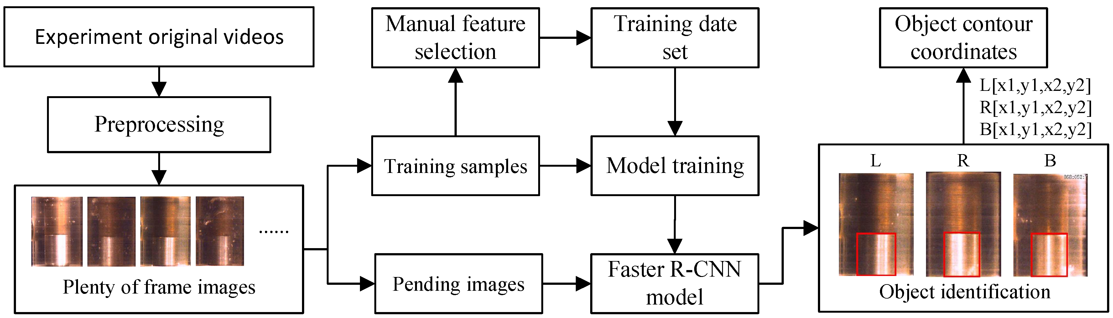
4. Algorithm Development

4.1. 2D Bubble Feature Detection

To extract the morphological data of the bubbles from the recorded experimental videos, we used the MATLAB software. The valve port area where the cavitating bubbles appeared was thoroughly analyzed by an image processing algorithm based on the frame differencing method. Obtaining the bubble feature data of bubbles from the images requires the pre-processing and the process is shown in Figure 5. The original images were converted to grayscale image using rgb2gray function in MATLAB software. The difference between two frames within a defined internal would be calculated. In addition, the result was converted to binary image (also called as BW image) using im2bw function in MATLAB software. As a result, the 2D bubble feature data can be obtained for further calculation.

Figure 6 presents the process for detecting the 2D feature of cavitation bubbles. The semi-major sizes of the cavitation bubble on the x, y, and z axes. The shape of the 2D bubble was defined as ellipse. In addition, the long or short axes of the ellipse are determined by the width (w) and height (h) of the detected area. Furthermore, the center of a bubble is estimated by the detected coordinate $(x_{lt},y_{lt})$, w and h:

$$\left\{\begin{array}{c}x=x_{lt}+0.5\times w,\hfill \\ y=y_{lt}+0.5\times h.\hfill \end{array}\right.$$

(5)

The center coordinate can be used to reconstruct the 3D motion parameters of bubbles afterwards. The 2D bubble features of the relative motion equalling the previous frame were extracted. Bubble clusters were assumed to be larger bubbles while those in developing or under collapsing mode were presumed smaller bubbles. The motion features in terms of the smallest pixel point were detected by the 2D cavitation bubble detection algorithm; the smallest discernable bubble size was restricted by the resolution of the video.

4.2. Feature Identification of the Opaque Object

The valve seat and core were manufactured by stainless steel materials. The brass material was used to compose the valve rod. Ultimately, it was separately distinguished by its color difference feature at the interface between the valve core and rod. A 3D coordinate system built by the mid-point of the boundary line between the valve core and the its rod to define the coordinates origin of the 3D model. The algorithm of the valve core identification was based on the Faster R-CNN method developed by Ren et al. [42], which is a mainstream deep learning method in object detection. Figure 7 illustrates the object detection model that is based on deep learning, requiring a large number of training samples. The detection accuracy meets the adequate requirements after processing the training model and the coordinates of the valve core contour were generated through the Faster R-CNN model. In addition, getting the valve core’s diameter in pixel scale and its real size ($r_{\mathrm{core}}=17$ mm), it is easy to transform the pixel value of the position of the bubbles into the actual size, whose unit is millimeters (mm).

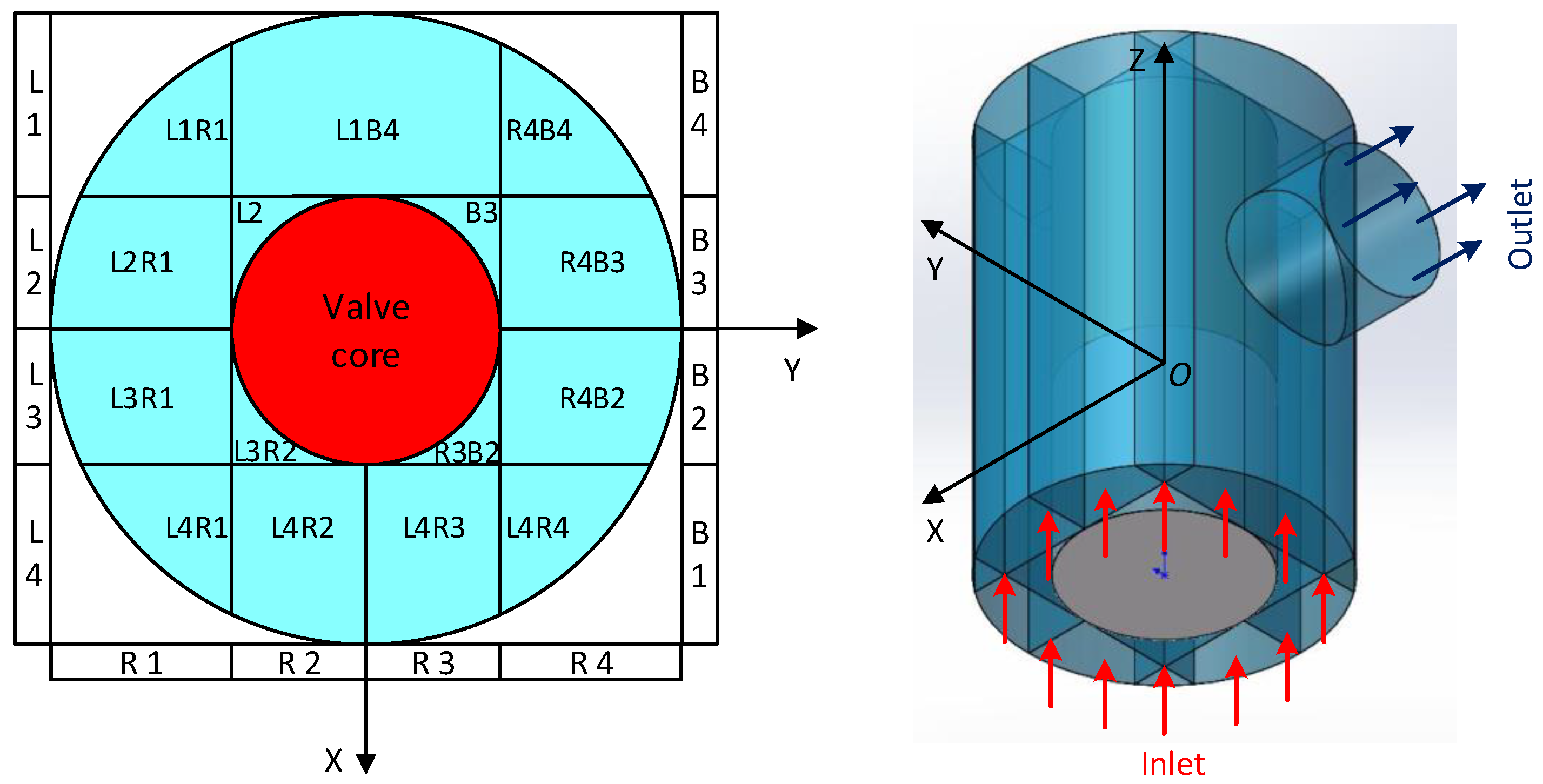
4.3. 3D Bubble Cluster Reconstruction

Reconstructing the 3D bubbles was simplified using the 3D Cartesian coordinates system. The origin of the model was determined from the contact surface of the valve core and the valve rod. From Figure 8b, the x and z axes in the left (L) side and back (B) side of the valve body represent the horizontal and vertical directions, respectively. It is worth emphasizing that the type of the space rectangular coordinate system is left-handed cartesian coordinate. And it is different with the x-y coordinate for optimization calculation. Due to different conditions of the mirror reflection, the positive x-axis of the L-side and the B-side was analogous. Concerning the right (R) side of the valve body, the y and z-axes were set in the corresponding horizontal and vertical directions. Additionally, the valve port area in Figure 9 was divided into 15 parts so as to decrease the matching scope and the possible associated errors. The left-handed Cartesian coordinates was used to express the spatial location of the reconstructed bubble.

The requirement of the 3D bubble cluster reconstruction was to match the bubbles from the different sides of the valve with the same bubbles in the 3D space. In addition, the bubbles y-axis values on the L and B sides were obtained from the B-side. The lack of vision from the R-side resulted the y-axis values of the bubbles belonging to the L2, L1B4, and B3 space to be fixed with a random value. The following equations illustrate the mathematical model of the bubble matching process:

$$D_{ij}=1+|Z_i-Z_j|,$$

(6)

where i and j are two bubbles on different sides. In addition, $Z_i$ and $Z_j$ are their coordinate values on the z-axis. $Z_i$ and $Z_j$ can be get through the 2D bubble detection results of Equation (5). The $Z_i$ and $Z_j$ are equal to the corresponding value of y in Equation (5). The index $D_{ij}$ is the difference of the z-axes regarding the two matching 2D bubbles:

$$H_{ij}=\frac{h_i}{h_j}+\frac{h_j}{h_i},$$

(7)

where $H_{ij}$ is termed as the height difference. In addition, $h_i$, $h_j$ are the height of the i and j frames, which can be also obtained according to the calculation results of the 2D bubble detection algorithm, as shown in Figure 8b:

$$M_{ij}=D_{ij}{H}_{ij},$$

(8)

where $M_{ij}$ is the marching index of the complete judgement of $D_{ij}$ and $H_{ij}$. If $M_{ij}$ is less than the $M_{max}$, the bubbles i and j are considered a probable 3D bubble. Prior to the pairs with the minimum $M_{ij}$ being designated as coordinating 3D bubbles, the bubbles from the three sides (L, R, and B) are matched. To simulate the bubbles (small ones, clustered ones) using the reconstruction algorithm, ellipses were used to extract their outer contours, as shown in Figure 8c.

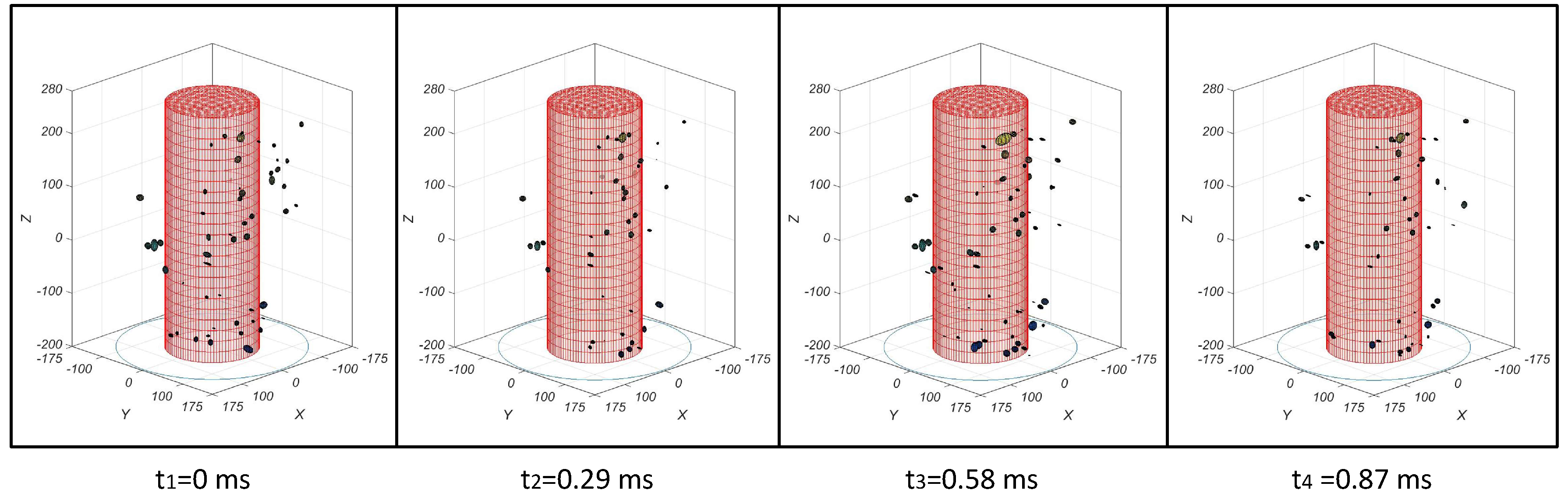
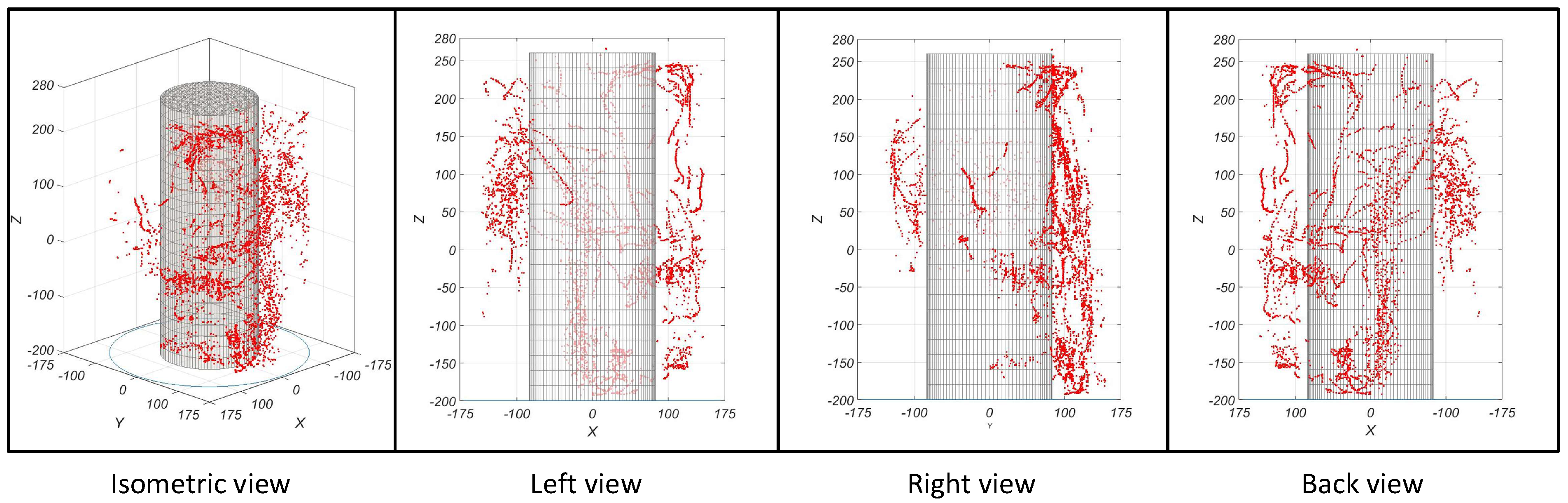
5. Results and Analysis

The flow profiles of the bubbles were analyzed based on the calculated results of the 3D bubble reconstruction algorithm. Figure 8c displays the size and distribution of the 3D bubbles recreated by computing and processing a certain frame from the recorded video. Stereoscopic parallax explains the following results: the bubble viewed in the mirror deviated from its actual appearance. Hence, the 3D bubble image from the back (B) side appeared to opposite left and right when compared with the mirror image of the B side in Figure 8a,b. As per the 3D reconstruction results, the bubble algorithm gave satisfying results. Even if not all bubbles were reconstructed, the results of the 3D reconstruction tallied with the original experimental images, thereby concluding with a vivid and solid reference for recreating the bubble morphology.

Figure 10 illustrates the 3D reconstructed bubble flow profile of four adjacent frames from 0 ms to 0.87 ms. The time interval between two adjacent frames was the least time difference captured by the high-speed camera, which was equal to 0.29 ms. Furthermore, the 3D bubble reconstruction algorithm was stable enough to simulate and evaluate the bubble flow profile in each frame.

As an example, a short experimental video which consisted of 50 frames of images was used to further analyze the characteristics of the reconstructed 3D cavitation bubble cluster. Its first four frames were the same frames in Figure 10. It is worth noting that the time of 50 frames of experimental images is only 14.5 ms, which exhibits the advantage of the high-camera camera. The number of 3D bubbles fluctuating within 50 frames of experiment images was showed in Figure 11, which can present the size of the bubbles and its number in each time interval The blue-color curve mainly floats between 40 to 70, which indicates that the generation and collapse of the cavitation bubbles can achieve a relative balance in a short time. The average number of bubble is 57.78.

The cavitation volume percentage in each frame is stated as Equation (9):

$$P_v=\frac{{\displaystyle \sum _{i=1}^n}\frac{4}{3}\pi a_i{b}_i{c}_i}{\pi (R_{\mathrm{fluid}}-r_{\mathrm{core}})h}\times 100\%,$$

(9)

where $R_{\mathrm{fluid}}$ is the radius of the fluid field in the valve and $r_{\mathrm{core}}$ is the radius of the valve core. In addition, $R_{\mathrm{fluid}}$ and $r_{\mathrm{core}}$ are constants. $a_i$, $b_i$, $c_i$ are the three semi-major sizes of the cavitation bubble on the x, y, and z-axes.

The variation of the cavitation volume percentage $P_v$ over time is shown in Figure 11. The change of the $P_v$ and the number of bubbles between the adjacent frames revealed that the growth and collapse of the cavitation bubbles were recurrent and fast. While comparing the $P_v$ curve with the number of bubble curve in Figure 11, an obvious positive correlation between the number of bubbles and the percentage of cavitation can be found. Moreover, the increase in the number of bubble and the $P_v$ did not exactly match; at times, while the cavitation volume percentage was decreasing, the number of bubbles did increase. Through the analysis of both results in Figure 11 and the original experiment images, it was concluded that scattering of the bubble clusters into small bubbles increased the number of bubbles in the cavitating space.

As shown in Figure 12, a short experimental video with 100 frames were analyzed. Various perspectives of the bubble clouds were presented and from the 100th frame (at about 29 ms), 5635 cavitation bubbles were detected and reconstructed, respectively. Based on the scatter diagram, the flow pattern of the 3D bubble cluster could be inferred. For example, the path and direction of the bubble flow were analyzed in Figure 13 through the presence of an obvious bubble headstream on the back side. The bubbles generated by this headstream were then separated into three paths (arrows)as shown in Figure 13. In addition, a large number of bubbles were flown out of the observed area through the outlet port, although there were certainly many that imploded and collapsed in the observed field.

Based on the calculated data of the bubbles’ space coordinates, the kernel densities of the bubbles on the x–y plane are shown in Figure 14. Almost all of the cavitation bubbles in the 100 frames are on the positive side of the y-axis. The high density around the point (0,100) validates the analysis of the bubble headstream. A maximum number of bubbles were detected by the algorithm that gave satisfying results as they were easily defined and selected across all the concerned fluid domain, as shown in Figure 8. The regions with the highest kernel densities in Figure 14 (output of the 100th frame) are based on the space partitions R4B4, R4B3, R4B2, and R4B1, respectively. Likewise, partition L1B4 represents the exit of the valve, which directly influences the flow in the partition L1R1 and R4B4, respectively. The bubble cluster rapidly shifted on the right side of the valve core within 29 ms due to the high velocity-low pressure zone (vortices) developed after the vena contracta formed soon after the fluid leaves the valve seat (the valve core opening was set to 1 mm).

6. Conclusions

Throughout this study, the optimal arrangement of the one-camera-five-mirrors module, the different algorithms applied in detecting the valve core and the bubbles morphology, and the reconstruction of the 3D bubble clusters along with the calculation of the cavitation volume percentage together provided favorable results. In addition, analysis of the recorded bubbly flow using the stable and effective algorithms in the transparent throttle valve proved to be ideal. Lastly, calculating the cavitation volume percentage broadened the concept of bubbles detection in the fluid flow, and it could be applied successfully in other cases as well.

References

1. Belden, J.; Ravela, S.; Truscott, T.T.; Techet, A.H. Three-dimensional bubble field resolution using synthetic aperture imaging: Application to a plunging jet. Exp. Fluids 2012, 53, 839–861. [Google Scholar] [CrossRef]
2. Ahmed, F.S.; Sensenich, B.A.; Gheni, S.A.; Znerdstrovic, D.; Al Dahhan, M.H. Bubble dynamics in 2D bubble column: Comparison between high-speed camera imaging analysis and 4-point optical probe. Chem. Eng. Commun. 2015, 202, 85–95. [Google Scholar] [CrossRef]
3. Lau, Y.M.; Deen, N.G.; Kuipers, J.A.M. Development of an image measurement technique for size distribution in dense bubbly flows. Chem. Eng. Sci. 2013, 94, 20–29. [Google Scholar] [CrossRef]
4. Zhang, Y.; Liu, M.; Xu, Y.; Tang, C. Three-dimensional volume of fluid simulations on bubble formation and dynamics in bubble columns. Chem. Eng. Sci. 2012, 73, 55–78. [Google Scholar] [CrossRef]
5. Tayler, A.B.; Holland, D.J.; Sederman, A.J.; Gladden, L.F. Applications of ultra-fast MRI to high voidage bubbly flow: Measurement of bubble size distributions, interfacial area and hydrodynamics. Chem. Eng. Sci. 2012, 71, 468–483. [Google Scholar] [CrossRef]
6. Zhao, L.; Sun, L.; Mo, Z.; Tang, J.; Hu, L.; Bao, J. An investigation on bubble motion in liquid flowing through a rectangular Venturi channel. Exp. Therm. Fluid Sci. 2018, 97, 48–58. [Google Scholar] [CrossRef]
7. Xia, G.; Cai, B.; Cheng, L.; Wang, Z.; Jia, Y. Experimental study and modelling of average void fraction of gas-liquid two-phase flow in a helically coiled rectangular channel. Exp. Therm. Fluid Sci. 2018, 94, 9–22. [Google Scholar] [CrossRef]
8. Fu, Y.; Liu, Y. Development of a robust image processing technique for bubbly flow measurement in a narrow rectangular channel. Int. J. Multiphase Flow 2016, 84, 217–228. [Google Scholar] [CrossRef]
9. Lomakin, V.O.; Kuleshova, M.S.; Kraeva, E.A. Fluid Flow in the Throttle Channel in the Presence of Cavitation. Procedia Eng. 2015, 106, 27–35. [Google Scholar] [CrossRef]
10. Gavaises, M.; Villa, F.; Koukouvinis, P.; Marengo, M.; Franc, J.P. Visualisation and les simulation of cavitation cloud formation and collapse in an axisymmetric geometry. Int. J. Multiphase Flow 2015, 68, 14–26. [Google Scholar] [CrossRef]
11. Kravtsova, A.Y.; Markovich, D.M.; Pervunin, K.S.; Timoshevskiy, M.V.; Hanjalić, K. High-speed visualization and PIV measurements of cavitating flows around a semi-circular leading-edge flat plate and NACA0015 hydrofoil. Int. J. Multiphase Flow 2014, 60, 119–134. [Google Scholar] [CrossRef]
12. Singhal, A.K.; Athavale, M.M.; Li, H.; Jiang, Y. Mathematical Basis and Validation of the Full Cavitation Model. J. Fluids Eng. 2002, 124, 617–624. [Google Scholar] [CrossRef]
13. Guevara-Lopez, E.; Sanjuan-Galindo, R.; Cordova-Aguilar, M.S.; Corkidi, G.; Ascanio, G.; Galindo, E. High-speed visualization of multiphase dispersions in a mixing tank. Chem. Eng. Res. Des. 2008, 86, 1382–1387. [Google Scholar] [CrossRef]
14. Tan, D.; Mi, J. High speed imaging study of the dynamics of ultrasonic bubbles at a liquid-solid interface. In Materials Science Forum, Proceedings of the 6th International Light Metals Technology Conference (LMT 2013), Old Windsor, UK, 24–26 July 2013; Trans Tech Publications Ltd.: Zürich, Switzerland, 2013; Volume 765, pp. 230–234. [Google Scholar] [CrossRef]
15. Jacobson, B.O.; Hamrock, B.J. High-speed motion picture camera experiments of cavitation in dynamically loaded journal bearings. J. Lubr. Technol. 1983, 105, 446–452. [Google Scholar] [CrossRef]
16. Dencks, S.; Ackermann, D.; Schmitz, G. Evaluation of bubble tracking algorithms for super-resolution imaging of microvessels. In Proceedings of the 2016 IEEE International Ultrasonics Symposium (IUS), Tours, France, 18–21 September 2016; pp. 1–4. [Google Scholar] [CrossRef]
17. Lauterborn, W.; Hentschel, W. Cavitation bubble dynamics studied by high speed photography and holography: Part one. Ultrasonics 1985, 23, 260–268. [Google Scholar] [CrossRef]
18. Lauterborn, W.; Hentschel, W. Cavitation bubble dynamics studied by high speed photography and holography: Part two. Ultrasonics 1986, 24, 59–65. [Google Scholar] [CrossRef]
19. Kent, J.C.; Eaton, A.R. Stereo photography of neutral density He-filled bubbles for 3D fluid motion studies in an engine cylinder. Appl. Opt. 1982, 21, 904–912. [Google Scholar] [CrossRef] [PubMed]
20. Racca, R.G.; Dewey, J.M. A method for automatic particle tracking in a three-dimensional flow field. Exp. Fluids 1988, 6, 25–32. [Google Scholar] [CrossRef]
21. Xue, T.; Qu, L.; Wu, B. Matching and 3D Reconstruction of Multibubbles Based on Virtual Stereo Vision. IEEE Trans. Instrum. Meas. 2014, 63, 1639–1647. [Google Scholar] [CrossRef]
22. Xue, T.; Xu, L.S.; Zhang, S.Z. Bubble behavior characteristics based on virtual binocular stereo vision. Optoelectron. Lett. 2018, 14, 44–47. [Google Scholar] [CrossRef]
23. Xue, T.; Qu, L.; Cao, Z.; Zhang, T. Three-dimensional feature parameters measurement of bubbles in gas-liquid two-phase flow based on virtual stereo vision. Flow Meas. Instrum. 2012, 27, 29–36. [Google Scholar] [CrossRef]
24. Xue, T.; Chen, Y.; Ge, P. Multibubbles Segmentation and Characteristic Measurement in Gas-Liquid Two-Phase Flow. Adv. Mech. Eng. 2013, 5, 143939. [Google Scholar] [CrossRef]
25. Mitra, A.; Bhattacharya, P.; Mukhopadhyay, S.; Dhar, K.K. Experimental study on shape and path of small bubbles using video-image analysis. In Proceedings of the 2015 3rd International Conference on Computer, Communication, Control and Information Technology, C3IT 2015, West-Bengal, India, 7–8 February 2015; Institute of Electrical and Electronics Engineers Inc.: Piscataway, NJ, USA, 2015. [Google Scholar] [CrossRef]
26. Acuña, C.A.; Finch, J.A. Tracking velocity of multiple bubbles in a swarm. Int. J. Miner. Process. 2010, 94, 147–158. [Google Scholar] [CrossRef]
27. Cheng, D.C.; Burkhardt, H. Template-based bubble identification and tracking in image sequences. Int. J. Therm. Sci. 2006, 45, 321–330. [Google Scholar] [CrossRef]
28. Krimerman, M. Reconstruction of Bubble Trajectories and Velocity Estimation. Master’s Thesis, The University of British Columbia, Vancouver, BC, Canada, February 2013. [Google Scholar] [CrossRef]
29. Bakshi, A.; Altantzis, C.; Bates, R.B.; Ghoniem, A.F. Multiphase-flow statistics using 3D detection and tracking algorithm (MS3DATA): Methodology and application to large-scale fluidized beds. Chem. Eng. J. 2016, 293, 355–364. [Google Scholar] [CrossRef]
30. Feng, X.F.; Pan, D.F. Research on the application of single camera stereo vision sensor in three-dimensional point measurement. J. Mod. Opt. 2015, 62, 1204–1210. [Google Scholar] [CrossRef]
31. Figueroa-Espinoza, B.; Mena, B.; Aguilar-Corona, A.; Zenit, R. The lifespan of clusters in confined bubbly liquids. Int. J. Multiphase Flow 2018, 106, 138–146. [Google Scholar] [CrossRef]
32. Fu, Y.; Liu, Y. Experimental study of bubbly flow using image processing techniques. Nucl. Eng. Des. 2016, 310, 570–579. [Google Scholar] [CrossRef]
33. Chakraborty, S.; Das, P.K. Characterization of bubbly flow through the fusion of multiple features extracted from high speed images. In Proceedings of the 2016 IEEE First International Conference on Control, Measurement and Instrumentation (CMI), Kolkata, India, 8–10 January 2016; pp. 1–5. [Google Scholar] [CrossRef]
34. De Langlard, M.; Al-Saddik, H.; Charton, S.; Debayle, J.; Lamadie, F. An efficiency improved recognition algorithm for highly overlapping ellipses: Application to dense bubbly flows. Pattern Recognit. Lett. 2018, 101, 88–95. [Google Scholar] [CrossRef]
35. Honkanen, M. Reconstruction of a three-dimensional bubble surface from high-speed orthogonal imaging of dilute bubbly flow. Int. J. Multiphase Flow 2009, 63, 469–480. [Google Scholar] [CrossRef] [Green Version]
36. Markus, H.; Pentti, S.; Tuomas, S.; Jouko, N. Recognition of highly overlapping ellipse-like bubble images. Meas. Sci. Technol. 2005, 16, 1760–1770. [Google Scholar] [CrossRef]
37. Zhang, W.H.; Jiang, X.; Liu, Y.M. A method for recognizing overlapping elliptical bubbles in bubble image. Patt. Recognit. Lett. 2012, 33, 1543–1548. [Google Scholar] [CrossRef]
38. Fujisawa, N.; Fujita, Y.; Yanagisawa, K.; Fujisawa, K.; Yamagata, T. Simultaneous observation of cavitation collapse and shock wave formation in cavitating jet. Exp. Therm. Fluid Sci. 2018, 94, 159–167. [Google Scholar] [CrossRef]
39. Kompella, V.R.; Sturm, P. Collective-reward based approach for detection of semi-transparent objects in single images. Comput. Vis. Image Underst. 2012, 116, 484–499. [Google Scholar] [CrossRef] [Green Version]
40. Hata, S.; Saitoh, Y.; Kumamura, S.; Kaida, K. Shape extraction of transparent object using genetic algorithm. In Proceedings of the 13th International Conference on Pattern Recognition, Vienna, Austria, 25–29 August 1996; Volume 4, pp. 684–688. [Google Scholar] [CrossRef]
41. Han, K.; Wong, K.Y.K.; Liu, M. Dense reconstruction of transparent objects by altering incident light paths through refraction. Int. J. Comput. Vis. 2018, 126, 460–475. [Google Scholar] [CrossRef]
42. Ren, S.; He, K.; Girshick, R.; Sun, J. Faster R-CNN: Towards real-time object detection with region proposal networks. arXiv. 2016. Available online: https://arxiv.org/abs/1506.01497 (accessed on 23 September 2018). [CrossRef] [PubMed]
Figure 1. Overall structure of the experimental setups.
Applsci 08 01783 g001
Figure 2. Experimental configuration for the 3D imaging of cavitation bubble.
Applsci 08 01783 g002
Figure 3. Schematic diagram of the 3D imaging principle.
Applsci 08 01783 g003
Figure 4. Establishment and parameter setting of the optimization model.
Applsci 08 01783 g004
Figure 5. Bubble feature extraction framework.
Applsci 08 01783 g005
Figure 6. Image processing of the 2D bubble feature detection algorithm.
Applsci 08 01783 g006
Figure 7. Block diagram of Faster R-CNN model. (R-CNN: region-based convolutional neural network).
Applsci 08 01783 g007
Figure 8. 2D Detection and 3D reconstruction results of the bubble cluster (unit: mm). (a) original images; (b) 2D detection results; (c) 3D reconstuction results.
Applsci 08 01783 g008
Figure 9. Space partition of the flow field.
Applsci 08 01783 g009
Figure 10. 3D reconstruction results of bubble flow in a short time (unit: mm).
Applsci 08 01783 g010
Figure 11. Change of the number of bubble and P v over time.
Applsci 08 01783 g011
Figure 12. Space distribution of the cavitation bubble cluster of 100 frames (unit: mm).
Applsci 08 01783 g012
Figure 13. Flow path of the bubble cluster from the back view (unit: mm).
Applsci 08 01783 g013
Figure 14. Kernel density of the cavitation bubbles on the xy plane.
Applsci 08 01783 g014