Research Progress of Visual Inspection Technology of Steel Products—A Review

Abstract

The automation and intellectualization of the manufacturing processes in the iron and steel industry needs the strong support of inspection technologies, which play an important role in the field of quality control. At present, visual inspection technology based on image processing has an absolute advantage because of its intuitive nature, convenience, and efficiency. A major breakthrough in this field can be achieved if sufficient research regarding visual inspection technologies is undertaken. Therefore, the purpose of this article is to study the latest developments in steel inspection relating to the detected object, system hardware, and system software, existing problems of current inspection technologies, and future research directions. The paper mainly focuses on the research status and trends of inspection technology. The network framework based on deep learning provides space for the development of end-to-end mode inspection technology, which would greatly promote the implementation of intelligent manufacturing.

1. Introduction

China’s iron and steel industry has made tremendous contributions to the development of its national economy. In recent years, the rapid rise in the output of steel products has been accompanied by a large number of defects, which could bring significant economic losses to enterprises, and ultimately affect their brand image. Therefore, it is necessary to study detection methods, particularly since artificial detection methods no longer meet the enterprise requirements regarding time, cost, and precision.

Visual detection technology based on image processing has been widely used in various fields, such as medicine [1], the iron and steel industry [2,3], art [4], the textile industry [5], and the automobile industry [6] for its unique advantages of intuition, accuracy, and convenience. Early detection methods for steel defects are classified as contact detection and non-contact detection [7]. The former receives information through direct contact with the sample surface by the sensing element of a contact-detection device. The latter is based on the technology of photoelectricity, and electromagnetism to obtain the parameter information of the sample surface without contacting it.

Contact-detection methods include magnetic particle testing (MPT) and liquid penetration testing (LPT). Although intuitive images can be quickly obtained via these methods, to do so is not practicable. Non-contact methods include ultrasonic scanning, electromagnetic testing, etc., in which ultrasound or electromagnetic signals are converted to optical signals. Results are not intuitive, but need to be judged by professionals.

Visual detection based on image sensors stands out from the range of non-contact detection technologies, because it is an effective combination of the high speed achieved with contact detection methods and the independence of non-contact detection methods. The key feature is that it can be implemented by using only a universal computer and a dedicated image processor. Indeed, the number of publications related to defect detection has grown rapidly over the past decade, which is a trend that may be due to the rapid advance of computing capacity, the enhancement of sensor performance, and the great improvement of image processing technology.

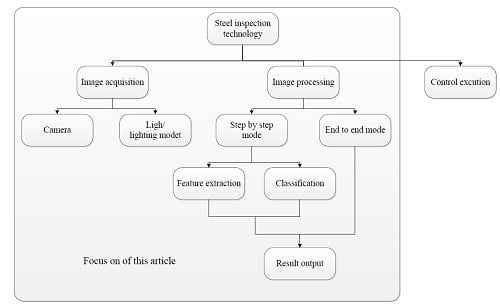
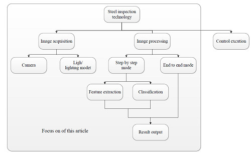
The basic components of a typical visual system are an image acquisition unit, an image processing unit, and a control execution unit (Figure 1). The image acquisition unit is the component of the system hardware, and its main task is to obtain high-quality images, since low-quality images lead to algorithm burden. Excellent visual software can quickly and accurately detect the target features in the image and minimize dependence on the system hardware. The sorting mechanism can adopt an electromechanical system or hydraulic system, but the dynamic characteristics (i.e., rapidity and stability) of the system are important. This paper focus on image acquisition and image processing units.

With the maturity of the basic theory of image analysis, the development of the detection field has advanced by leaps and bounds, and several reviews of defect detection have been undertaken. Commercially available inspection equipment and visual inspection systems, as well as practical applications of visual inspection, are summarized in Chin [8], Newman, [9]. Amongst recent literature reviews, a large number of methods and techniques for the free surface detection of parts are studied in Li [10]. Development trends of visual inspection are presented in article Shirvaikar [11], which mainly focuses on the introduction of visual detection systems relating to hardware and software, but detailed algorithm comparisons are not provided. Reviews of visual detection in the manufacture of textiles Hanbay [12], food, and agriculture Jfs [13] have also contributed to the development of detection technology. However, because the reflective properties of steel products (55–65%) [14] differ between foods and fabrics, these testing methods are for reference only. Notably, a comprehensive review of defect detection in steel surfaces has been conducted Neogi [15], and is a valuable article for researchers in the field. However, the chronological distribution of the references in Neogi [15] suggests that it is somewhat dated, with 13.82% of references from before 2000, 65.5% from 2001–2010, and 20.68% from after 2010. In contrast, the chronological distribution of references in the present paper—10.41% from prior to 2000, 37.5% from 2000–2010, and 52.08% from after 2010—indicates that it is more up-to-date with the latest technological developments. Thus, it is intended that the present study provide a supplement to Neogi [15].

In Section 2, the types of steel products and common defects are presented, so as to understand the complexity and diversity of visual detection. In Section 3, the hardware composition of inspection systems is explained. Detection and classification methods are reviewed according to different theories in Section 4 and Section 5. In Section 6, a literature analysis is conducted, which includes not only an analysis of detection technology, but also an analysis of the scale of the detection market. Conclusions and further prospects are provided in Section 7.

2. Types of Defects in Steel Products

The wide variety of steel products can be roughly divided into two categories: flat products and long products (Figure 2).

Steel products have been identified as having 55 types of defects Neogi [15]; Figure 3 shows some examples.

The wide range of defects can be classified according to the general type of steel product as follows in

Table 1. Common defect types of different steel products.

Steel Type	Type of Defect	References
Billet	Cracks, scratches	[17,18,19,20,21]
Hot strip	Cracks, longitudinal scratches,	[16,22,23,24,25,26,27,28,29,30]
	transverse scratches, scales,
	delamination, roll marks,
	pit defects, seams, inclusions
Cold strip	Bruises, slags, inclusions, seams, oxide scales, cracks, holes, feather roll marks,	[31,32,33,34,35,36,37,38,39,40,41,42,43]
	Latex marks
Stainless steel	Slag inclusions, scratches in pickling,	[44]
	scratches
Rod/bar	Cracks, scratches	[45,46,47,48,49]

.

Establishing a defect detection system is not easy. In order to create a reliable and repeatable test system, produ ct manufacturers often need to work with test engineers to conduct qualitative and quantitative analyses of potential defects. Defects can be roughly divided into three situations:

(1)

In most cases, defects can be easily detected by using standard imaging tools. For example, pinholes Liu [31] and certain impurities are usually round, and pixels that appear bright on an image fall on a dark background, or vice versa, so are easily discernible.

(2)

A slightly more complex situation is that the defect definition, including its size and shape, are not very clear, but it can still be distinguished from the underlying background. This situation mainly includes wear, or slender, low-contrast linear defects Yun [17]. Examples are scratches Dupont [18] and cracks Choi [50] on products. These types of defects may require more advanced imaging detection tools.

(3)

The most complicated case is a defect in which its definition, size, and shape are not clear, and there is no recognition mode, so that it is difficult to distinguish the defect from the underlying background. This kind of situation mainly includes printing defects and some random medium “impurities” which pose significant challenges to detection technology.

3. The Hardware Composition of the Inspection System

3.1. Camera

An industrial camera is at the core of the system hardware. The frame rate (the rate at which the camera collects and transmits images) and resolution are two important parameters of the camera. The frame rate must be greater than the detection speed; 10 fps is usually sufficient to meet industrial requirements. The required resolution depends on the size of the features relative to the overall image. For example, suppose the surface scratch of an object is detected, the size of the object to be photographed is a × b mm, and the detection accuracy is 0.01 mm. Then, the minimum resolution formula of the camera can be determined as:

$$(a/0.01)\times (b/0.01)=Resolution$$

(1)

Industrial cameras are divided into two types according to the differences of the image sensors: charge coupled devices (CCD) and complementary metal oxide semiconductor devices (CMOS) Koller [51]. The differences are as follows.

(1)

Different imaging processes: A CCD utilizes a small number of output nodes to output data uniformly, thereby ensuring good signal consistency. By contrast, each pixel in a CMOS chip has its own signal amplifier, with charge conversion done separately, so output signal consistency is poorer and more greatly affected by signal noise than with a CCD. However, a significant advantage of CMOS is low power consumption.

(2)

Different integration: The CCD manufacturing process is complex, and the output of a CCD consists only of an analog electrical signal, which requires a decoder, analog converter, and image signal processor. As a result, a CCD has low integration. A CMOS, on the other hand, can collect signals with an analog-to-digital converter on a chip with high integration and low cost. With the advancement of CMOS imaging technology, CMOS will have greater applications in the future.

(3)

Different image output speed: A CCD adopts photosensitive outputs sequentially, relatively slowly. With a CMOS, each charge element has its own switch controller, and the readout speed is very fast. Most high-speed cameras with a frame rate greater than 500 fps use CMOS.

(4)

Different noise levels: CCD technology is mature, and the imaging quality is superior to that of CMOS. CMOS has a higher degree of integration, a closer spacing distance, and more interference.

As part of so-called Industry 4.0, factories around the world are developing automation and intelligence, in which smart sensors play an important role. The smart camera Lee [52] has the functions of processor, memory, communication interface, operating system, etc., which can process a large amount of data in advance and assist subsequent automatic detection and judgment. Nguyen et al. [53] noted an ultra-high-speed silicon image sensor. The test chip of this image sensor realizes a temporal resolution of 10 ns. For a silicon image sensor, the limit is 11.1 fps. Considering the theoretical derivation, this high-speed image sensor can reach a frame rate near the theoretical limit.

3.2. Light Selection

Lighting devices will vary because of different operating environments. For hot rolled steel, the strip itself is a luminous heating element. In order to reduce the interference of internal light sources, the intensity of the light source should be much higher than that of the steel strip. Thus, the light source can only have high-power, long-distance characteristics, so that it can provide high-intensity light at a long distance. For the cold rolling environment, although the relative distance between the light source and the steel strip is short, a more continuous light is needed to attenuate unstable infrared light, in order to ensure the highest sensitivity of the lens to the visible light spectrum. Overall, high strength, life span, design freedom, heat radiation, and response speed should be considered during lighting arrangement.

At present, some classical light sources are optical fiber, LED (light-emitting diode) lights, and stroboscopic xenon lamps. Among the latter, the strobe xenon lamp is mainly used in the area array CCD detection system as shown in Figure 4a, since it can effectively deal with adverse environmental conditions, such as fog Luo [22].

An example of an optical fiber light source is the halogen lamp (Figure 4b), which is used in conjunction with a color filter adapter. The output of light through the cylinder prism can avoid overflow and increase light intensity by 10% Wu [54], which can result in an ideal performance if high-power halogen lamps are used in industrial sites. However, halogen lamps are not suitable for hot-rolled steel in poor environments, and are mainly used in the testing environments of cold-rolled steel and finished products because of their high price and susceptibility to damage.

LED lamps (Figure 4c) are a spontaneous radiation source. Spontaneous radiation is a process in which an excited atom spontaneously transitions from a high-energy state to a low-energy state, emitting a photon at the same time. LED lamps have the advantages of non-related light, no optical resonator, long lifespan, and easy maintenance. However, the weaknesses of the lamps are their narrow spectral range and that the wavelength is affected by the materials. The lifespan of LED lamps will also shorten as the ambient temperature increases, so they are not suitable for high-temperature applications. In addition, LEDs cannot be directly connected in parallel. Therefore, a method of a single-channel serial multi-channel parallel connection method is used to form an array LED, which then forms a light source through the prism. Owing to its low cost and long lifespan, LED light sources are usually equipped with cooling devices for hot-rolled inspection.

3.3. Lighting Method Selection

In addition to the influence of the light source and CCD sensor on detection effects, the lighting mode has a greater impact on the detection effect of steel products. Usually, lighting can be divided into light and dark lighting.

The bright field lighting method is shown in Figure 5a. In this mode, the light source and the CCD are on the same side of the strip. The light emitted by the light source enters the camera after being reflected by the detection target. The reflection angle β is equal to the incident angle α, and the line between the CCD sensor and the image of the light source must be on the same line as the reflected light.

The reflected light is evenly distributed on each area of the CCD sensor when there is no defect on the surface. However, reflected light at the defect position will change when a defect exists, and the illuminance entering the CCD sensor will be weakened. Therefore, the reflection of light in the defect area is altered for three-dimensional defects, and the illuminance of the defect position into the CCD sensor is less than the background light entering the CCD sensor; that is to say, the defect image is darker than the background image. As for two-dimensional defects, the reflection of the defect does not change, but two-dimensional defects are usually of different shades. The light in the darker region absorbs more light; therefore, the gray value of the defect image is higher than the background image when the defect color is lighter than the surface color of the strip. Conversely, the grayscale value of the defect image is lower than the background image when the color of defects is darker than the color of non-detects.

Therefore, the use of bright field lighting can not only detect two-dimensional (2D) defects, it can also detect three-dimensional (3D) defects. However, it is worth noting that the results will be significantly affected if a large fluctuation of the steel strip leads to exceeding the range of the reflection angle. Overall, the bright field method is more appropriate for detecting a type of defect that reflects and absorbs light, especially dark targets with a bright background, such as scales, oxide skins, pits, water marks, etc.

In the dark field lighting method (Figure 5b), the light source and the CCD sensor are also on the same side of the strip. In this case, the reflection angle β is not equal to the incident angle α, and the line between the CCD sensor and the image of the light source is not on the same line as the reflected light; therefore, it is difficult for light to enter the CCD sensor. Only when three-dimensional defects exist on the strip surface will the defect change the reflective nature of the light into a diffuse reflection. Then, the camera is able to collect some diffuse light, and the light from the defect position will be stronger than from areas without a defect. In addition, the light source itself has a collection effect of high-intensity light. Even if the incident angle is changed, it has little effect on the illumination of reflected light on CCD sensors. As a result, the CCD can still effectively detect a surface defect when the surface of the strip steel generates vibration. On the whole, the dark field lighting method is more suitable for the type of defects that can emit diffuse reflected light on the surface of a bright steel plate, and, in particular, bright targets with dark backgrounds, such as skins, pits, and indentations. There is a certain degree of tolerance to the vibration of the detection point.

The bright and dark double field lighting mode (Figure 5c) addresses the problems of detection of two-dimensional defects in dark field lighting and vibration at the detection point. However, this method has a high requirement for a high-intensity concentrated light effect of the light source; that is to say, the part of the dark field detection that is included will not be ideal if the concentrated light effect is not strong.

Overall, the appropriate light source and lighting mode allow us to capture the features of the object more accurately and improve the contrast between the object and the background. In this way, high-quality images can be obtained, and good detection results can be achieved.

4. Detection Methods

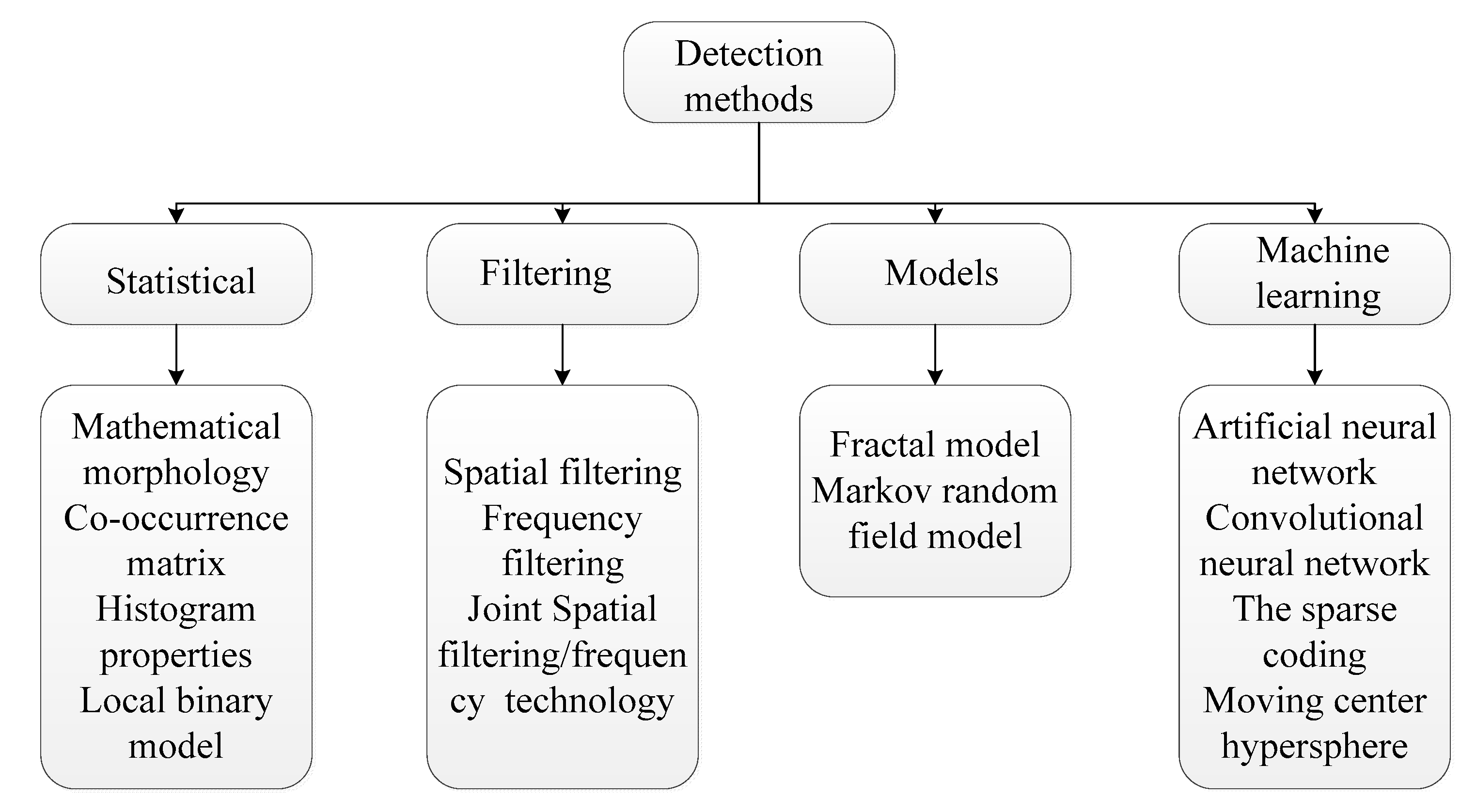
The performance of the software algorithm directly determines the result of detection. The detection task is arduous and challenging due to similarities between classes of defects and diversity within the classes. Due to this, domestic and foreign scholars have conducted significant research regarding steel inspection. Publications of the past 30 years can be classified according to basic theories, as shown in Figure 6.

4.1. Statistics

The statistical method is to establish a mathematical model using probability theory and mathematical statistics, which can be used to infer, predict, quantitatively analyze, and summarize the spatial distribution data of pixels. As a result, it can provide a basis and reference for subsequent decision-making. In the statistical method, the spatial distribution of gray values is defined with various forms of characterization, such as mathematical morphology, the co-occurrence matrix, histogram properties, and local binary models. These methods are widely used in the field of visual inspection.

Table 2. Strengths and weaknesses of statistical detection methods for steel defects.

Method	Strengths	Weaknesses
Mathematical morphology	Computational simplicity.	Morphological operations are only implemented on non-periodic steel defects.
	Geometric representation of texture images.
	Highly suitable for random or natural textures.
Co-occurrence matrix	Extracting spatial relationship of pixels with different statistical computations.	Difficult to judge the optimal displacement vector.
	High accuracy rate.
Histogram properties	Translation and rotation invariance.	Low detection rate (50–70%) for irregular textures.
	Calculation is simple.	Sensitive to noise.
Local binary pattern	Calculation is simple.	Too dependent on the gray value of the center point pixel.
	Recognition ability is strong.
	Rotation invariance and gray invariance.

compares defect detection methods based on statistics.

4.1.1. Mathematical Morphology

Mathematical morphology is a subject of image analysis based on lattice theory and topology. The basic operations include: corrosion and expansion, open and closed operations, skeleton extraction, limit corrosion, hit-and-miss transformation, morphological gradient, top-hat transformation, particle analysis, and watershed transformation. The cost matrix theory based on mathematical morphology, combined with the K-nearest neighbor (KNN) classifier, has been shown to detect eight defects of flat steel products in Dopont [18].

In Yun [19], Liu [23], Zheng [55], a genetic algorithm combined with mathematical morphology was adopted to realize the defect detection of steel products. In particular, Liu [23] studied an enhancement operator based on mathematical morphology (EOBMM), combined with a binarization method based on genetic algorithm (BMBGA), which can effectively overcome the effects of non-uniform illumination and enhance the detailed information of the image. A method using mathematical morphology in combination with filtering methods was described in Wu [24]. There are other, similar combinations; for example, mathematical morphology can be combined with the curvelet transform or the Gabor transform. Mathematical morphology in conjunction with the curvelet transform has been used for the detection of metallic surfaces Cord [56]. A morphological operation combined with an optimized Gabor filter method was derived to address the problem of detection performance decreasing due to billet shape, multiple defects, and scales Yun [57]. There are also studies on morphological methods Nguyen [53], Wu [54]. .

4.1.2. Co-Occurrence Matrix

The spatial gray level co-occurrence matrix was first proposed by Haralick [58], and it is a popular texture analysis method belonging to second-order statistics, which is defined by the joint probability density of two positional pixels. Texture features derived from the co-occurrence matrix (energy, entropy, contrast, uniformity, deficit moment, and correlation) have been used in various surface defects detection methods. The detection and classification of defects can be realized by extracting the spatial features of a gray-level co-occurrence matrix (GLCM) in combination with a classifier Yu [32].

4.1.3. Histogram Properties

Image histograms are widely used in various fields of image processing, because they have low computational cost and many other advantages, such as image translation, rotation, and scale invariance, specifically in the fields of threshold segmentation of grayscale images, image retrieval, and image classification based on color. There are many histogram statistics, four of which (mean, standard deviation, variance, and median) are the most frequently used as texture features. Liu et al. [59] performed a multivariate discriminant function based on a statistical histogram to model, and used three statistical characteristics—the deviation (Dg), the mean (mg), and the variance (Vg)—to represent the shape of a point. In Luo [22], they also adopted a method that selected a suitable threshold based on the histogram to extract features. In Martins [33], a study of principal component analysis combined with histogram statistics were presented.

4.1.4. Local Binary Pattern

The local binary pattern (LBP) is an operator that describes the local texture features of the image with rotation invariance and grayscale invariance. It is worth mentioning that the application of the LBP in classification recognition generally uses the statistical histogram of the LBP feature spectrum as the feature vector rather than the LBP feature spectrum itself. In order to improve the recognition rate, a new feature descriptor known as the adjacent evaluation completed local binary pattern (AECLBP) was proposed by Song et al. [16] for hot-rolled steel strip detection. In a recent study, an LBP operator with symbol and size, combined with a histogram and shape and distance statistic features, were developed by Chu et al. [60]. On one hand, this method can solve multi-class classification problems; on the other, it also has an anti-noise ability and high classification efficiency. On the whole, the LBP method performs better than the co-occurrence matrix and filtering methods in accurately detecting the surface texture defects of steel.

4.2. Methods Based on Filtering

Most of the methods discussed in this section have the common feature that they apply a filter bank to an image to calculate the energy of the filter response. These methods can be divided into the spatial domain, frequency domain, and joint spatial/frequency analysis methods.

Table 3. Strengths and weaknesses of filtering-based detection methods for steel defects.

Name	Strengths	Weaknesses
Spatial domain	A more centralized text-based approach (in which the segmentation of the text file is separate from the image).	Difficult to determine the optimal filter parameters.
		High computation cost.
Frequency analysis	Spatial frequency spectrum is invariant to shift, rotation, and scaling.	Lack ability of spatial orientation.
	Suitable for the detection of global and local defects.
		Not suitable for random texture detection.
	FFT (Fast Fourier transform.) calculation time is short (600 pixels with 2.2 ms).
Gabor Transform	Suitable for high dimensional feature space.	Difficult to determine the optimal filter parameters.
	An adaptive filter selection method is implemented to reduce the computational complexity.
		No rotation invariance.
	Suitable for defect detection in airspace and frequency domain.
Wavelet transform	Suitable for multi-scale image analysis.	Easily to be affected by feature correlations between the scales.
	High detection rate (83–97%).
	Efficient image compression with less information loss.
Multiscale Geometric Analysis	Suitable for the optimal and sparse representation of high-dimension data.	Redundancy problem (i.e., repeated data in a data set) cannot be solved.
	Good at image processing of strong noise background.
	Compression with less information.

compares filtering-based detection methods.

4.2.1. Spatial Domain

Spatial filtering is an enhancement method based on neighborhood processing that directly conducts operations in the two-dimensional space where the image is located. The most common operation of spatial filtering is template arithmetic, and the basic idea is to use the value of a pixel as a function of its own gray value and the gray value of its neighboring pixels. In spatial filtering, the gradient filters are mainly used to detect edges, lines, and isolated points. Sobel, Robert, Canny, Laplacian, and Deriche filters are popular tools for measuring edge density. Dupont et al. provided a method that used the Prewitt filter to extract edge information and realize defects of sheet products [18]. Guo et al. [61] used the Sobel gradient edge detection operator combined with the Fisher discriminant to detect defects on steel surfaces. Spatial filtering methods are also discussed in the literature [25,34,35,45,46,62,63,64] for the defect detection of various steel products. For the optical properties of highly reflective surfaces of cold-rolled strip, Zhao et al. [36] adopted a kind of homomorphic filtering algorithm based on a partial differential equation (PDE). Recently, the application of filter banks has been expressed in Bulnes [46], Liu [65], Li [47], and particularly in Li [47], which used mean filtering combined with a local annular contrast (LAC) detection method, which led to better performance.

4.2.2. Frequency Analysis

To address the limitation of spatial filtering methods (i.e., the kernel cannot be found in the defect image), the frequency domain analysis method was derived. This method firstly converts the image into frequency domain signals using the Fourier transform, and secondly performs a filtering analysis of the signals, and finally converts the signals back to the spatial domain to be stored by inverse Fourier transform. Three articles [25,37,38] were published successively, outlining the methods of frequency domain analysis for the defect detection of cold-rolled and hot-rolled steel. Among them, the method proposed in Wu [25] is the most effective, with a detection rate of up to 92.68%. They proposed a method of fast Fourier transform (FFT) combined with a local border search algorithm (LBSA) for the detection of hot-rolled steel strips.

4.2.3. Joint Spatial/Frequency Analysis Methods

Gabor Transform

Since the Fourier transform lacks spatial localization ability, it has a poor performance in practical applications. In order to solve this problem, the windowed Fourier transform was developed in 1946; this is known as the Gabor transform if the window function is a Gaussian function. Yun et al. [19] applied a Gabor filter optimized by genetic algorithm (GA) for the detection of corner cracking and thin cracking defects. Jeon et al. [66] adopted the Gabor filter to perform edge-pair detection in order to reduce the influence of lighting conditions, with satisfactory effects. D. Choi et al. [67] used a Gabor filter with morphological defect detection algorithms to detect pinholes on the surface of the steel plate. Choi [50] employed Gabor filtering and dual-threshold segmentation detection methods for the crack detection of steel plates. Among these methods, Choi [50] achieved the best results, with a detection rate of up to 94.43%.

Wavelet Transform

The Gabor transform is not adaptive, because the sliding window function is fixed once selected. On the contrary, the wavelet transform has a time-frequency window that can be adjusted; that is, the width of the window changes with the frequency. Thus, it overcomes the limitation of the Gabor transform. Wavelet transform was first put forward in 1974. The method was first used for defect detection Kaya [44] in 1995, because of the poor performance in diagonal detection using traditional edge-detection methods. Soon after, there were a lot of extensions of the method based on wavelet transform, such as the snake projection wavelet algorithm Li [68], undecimated wavelet transform algorithm [17], wavelet transform to obtain the approximate sub-image method Zhang [48], three-layer Haar wavelet feature set method Ghorai [26], discrete wavelet transform combined with adaptive local binarization method Yun [49], wavelet filtering in combination with center-surrounding difference method Xu [69] and, recently, anisotropic diffusion filter based on wavelet transform method [31]. The characteristics of wavelet transform are presented incisively and vividly in a large number of publications.

Multiscale Geometric Analysis

The excellent characteristics of wavelet transform in one-dimensional data analysis cannot be simply extended to two-dimensional or multi-dimensional data, because it cannot make full use of the unique geometric features of the data itself in the case of higher dimensions. Thus, it is not the optimal or the sparsest method for function representation. The multi-scale geometric analysis (MGA) method arose in response to the proper time and conditions, and typical representations of multi-scale geometric analysis appeared. Ridgelet transform Candès [70], wedgelet Claypoole [71], beamlet Donoho [72], curvelet Candès [73], bandelet Pennec [74], and contourlet Do [75] were successively proposed.

Zhang [27] studied a new image fusion method using bandelet transform based on MGA. In this method, a low-pass subband coefficient of a source image by bandelet transform is inputted into a pulse-coupled neural network (PCNN), and the fused image can then be obtained through inverse bandelet transform using the coefficient and geometric flow parameters. Ai et al. [20] applied the curvelet transform to decompose the image combined with Fourier transform to extract features. Xu et al. [76] explored a method of MGA based on the non-symmetry and anti-packing model (NAM). This method can adaptively be applied to three types of steel products—continuous casting slabs, hot-rolled steel, and cold-rolled steel—that cannot be assessed by the traditional method.

It can be seen from the theoretical development of signal analysis methods that Fourier analysis is especially suitable for analyzing stable signals over a long period of time. The Gabor transform has its own application, but its effect depends on the window function. Wavelet analysis is especially suitable for analyzing mutated and singular signals. Multi-scale geometric analysis is suitable for the “sparse” function representation of high-dimension data.

4.3. Method Based on Model

4.3.1. Fractal Model (FM)

The fractal model (FM) was first derived by Mandelbrot [77] in 1983. Fractal dimension and porosity are the most important metrics in a fractal model. The former is a measure of complexity and irregularity, while the latter represents structural change or unevenness. In 2008, Blackledge et al. [78] used a membership function to analyze the partial structure and fractal features of images for extracting new information. Yazdchi et al. [79] researched a multifractal-based segmentation method to locate defects, and then extracted 10 features, such as multi-dimensional fractal dimension, variance, mean value, and maximum value in the principal component vector to achieve defect detection. The method achieved accuracies of 97.9%.

4.3.2. Markov Random Field Model

One of the main uses of the Markov random field (MRF) model in image processing is image segmentation, which is the technology and process of dividing the image into several specific and unique regions and extracting the target of interest; hence, it is a key step between image processing and image analysis.

In MRF, two random fields are often used to describe the image. One is the labeling field, which is often called the implicit random field. The prior distribution is used to describe the local correlation of the label field. The other is the grayscale field or feature field. The distribution function is often used to describe the distribution of observation data or feature vectors under the condition of the labeling field. The process of obtaining feature vectors is the process of detection.

Based on Bayesian theory, MRF turns the image segmentation problem into a process of obtaining the maximum probability density. The formula is as follows:

$$P(W|S)=\frac{P(S|W)P\left(W\right)}{P(S)}$$

(2)

where $P\left(W\right)$, $P(S)$, and $P(S|W)$ are the prior probability, fixed value based on the observed value, and conditional probability distribution based on the observation S (also called the likelihood function), respectively. Then, the problem is converted into finding the maximum value of $P(S|W)P\left(W\right)$. The Markov random field was used as a texture analysis method, which was combined with a KNN classifier to achieve six kinds of steel surface defects detection, with classification rates of 79.36–91.36% Ünsalan [80].

Table 4. Strengths and weaknesses of model-based detection methods for steel defects.

Name	Strengths	Weaknesses
Fractal model (FM)	Remain invariant to large geometric transformations and lighting variations.	Low characteristic dimensions lead to weak judgment.
Markov random field model	Can be used with statistical and spectral methods for segmentation applications.	Not invariant to rotation and scaling.
		Cannot detect small defects.
		Not suitable for global texture analysis.
	Captures the local texture orientation information.
		Strong spatial constraint.

shows the comparison of model-based detection methods.

4.4. Method Based on Machine Learning

4.4.1. Artificial Neural Networks

Since 1980, artificial neural networks (ANN) have been a hotspot in the field of artificial intelligence. ANN abstracts the human brain neural network from the perspective of information processing to establish a simple model, and can then be used to form different networks according to different connection modes to achieve various functions (Figure 7). As early as 2000, Caleb [28] proposed an adaptive learning classification for surface defects of hot-rolled steel, and the average percentage classification accuracy was 84% for training data and 64% for test data. Later, an improved BP (Back propagation) algorithm based on error function was mentioned in Peng [39] to conduct the surface quality inspection of cold-rolled strip. Zhao [81] came up with an improved BP algorithm based on singular value decomposition and a generalized inverse matrix for five common defects (cracks, oxide, skin, holes, and scratches) of steel plate, overcoming the slow training of the traditional BP algorithm, with results showing that it could meet real-time requirements.

4.4.2. Convolutional Neural Network

Convolutional neural networks (CNNs) belong to a branch of ANN. As a network structure with fewer layers, ANNs have limited representation ability for complex functions, and generalization ability for complex classification problems is restricted to some extent. However, CNNs can realize complex function approximation by learning a deep nonlinear network structure. The deep neural network (DNN) has more layers (8–152 layers) than ANN, and needs more training data (4000–10,000 images).

An end-to-end detection network model was outlined in Yi [40]. Since the feature detection layer of CNNs is learned by training data, explicit feature extraction is avoided when using CNNs, while implicit learning is carried out from the training data. Moreover, since the weights of neurons on the same feature mapping surface are the same, the network can learn in parallel. It is worth mentioning that the detection accuracy is 99.29%. The CNN’s structure for surface defect recognition model is presented in

Table 5. Convolutional neural networks (CNNs) structure for surface defect recognition model (reproduced from Yi [40]).

Layer Type	Filter Size	Volume Size
Input	N/A	(3,144,144)
Convolution	(5,5)	(32,140,140)
Max pooling	(2,2)	(32,70,70)
Convolution	(5,5)	(32,66,66)
Max pooling	(2,2)	(32,33,33)
Convolution	(4.4)	(64,30,30)
Max pooling	(2,2)	(64,15,15)
Convolution	(4,4)	(64,12,12)
Max pooling	(2,2)	(64,6,6)
Convolution	(3,3)	(128,4,4)
Max pooling	(2,2)	(128,2,2)
Fully connected	N/A	(256)
Fully connected	N/A	(512)
Softmax	N/A	(7)

. In a recent study, Park et al. [82] employed CNNs to detect several types of defects on textured and non-textured surfaces, which was difficult to achieve by traditional machine learning methods. The recognition rate was 98%, and the time consumed for single image recognition was 0.01135 s. Masci et al. [21] proposed a max-pooling convolutional neural network method for the classification of steel defects. Compared with the commonly used support vector machine (SVM) classifier for feature descriptor training, this method can not only obtain better detection effects, it can also be directly used to detect the original image and segmentation defects, avoiding further time consumption and difficulty in optimizing adaptive preprocessing. However, changes in image size in a particular classification task have not yet been addressed by standard CNNs; nevertheless Masci et al. [41] put forward the multi-scale pyramidal pooling network, which had three characteristics: (1) a pyramidal pooling layer that made the net independent of input image size; (2) multi-scale feature extraction; and, (3) an encoding layer emulating standard dictionary-based encoding strategies. Hence, the problem of image scale in traditional CNNs was solved.

4.4.3. Moving Center Hypersphere

The moving center hypersphere (MCH) is a way to compress a reference sample. The basic idea of the MCH is to use a hypersphere to represent a cluster of points to approximate each sample with a number of hyperspheres. The center of the hypersphere is then moved, and its radius is expanded so that it should contain as many sample points as possible, and ultimately contain all of the sample points in the space. Two recent articles fully illustrate the novelty of this method. In 2017, a method with quantile hypersphere based on machine learning (QH-ML) was employed in Chu [83] for six kinds of defects on a steel surface. Soon after, in 2018, a defect classification model was established in Gong [84], which was a multi-hypersphere support vector machine (MHSVM) with additional information. It is not hard to see that this method has good generalization ability.

4.4.4. Sparse Coding

A sparse coding algorithm is an unsupervised learning method. The purpose of the sparse coding algorithm is to find a set of overcomplete base vectors φ, so that we can represent the input vector x as a linear combination of these base vectors:

$$x={\displaystyle \sum _{i=1}^k{a}_i{\varphi }_i}$$

(3)

where a is the weight. In reference Liu [85], the method of sparse coding was adopted to achieve defect detection.

Table 6. Strengths and weaknesses of machine learning-based detection methods for steel defects.

Name	Strengths	Weaknesses
Artificial neural networks	Real-time performance suitable for industrial application.	Large-scale feature vectors lead to high calculation cost.
	Can learn complex nonlinear input-output relationships.	Need lots of data (100–4000 images).
Convolutional neural network	End-to-end mode (raw image input, classification results output).	Large data sets are required (4000–10,000 images).
	High detection rate (95–100%).
Moving center hypersphere	Not sensitive to noise.	Optimal choice of parameters is difficult.
	High classification accuracy and efficiency (93–96%).
Sparse coding	Can be used not only in the input phase, but also in the output phase.	The calculation time is too long (more than 45.6 s [85]) to allow real-time detection.

shows the comparison of defect detection methods based on machine learning.

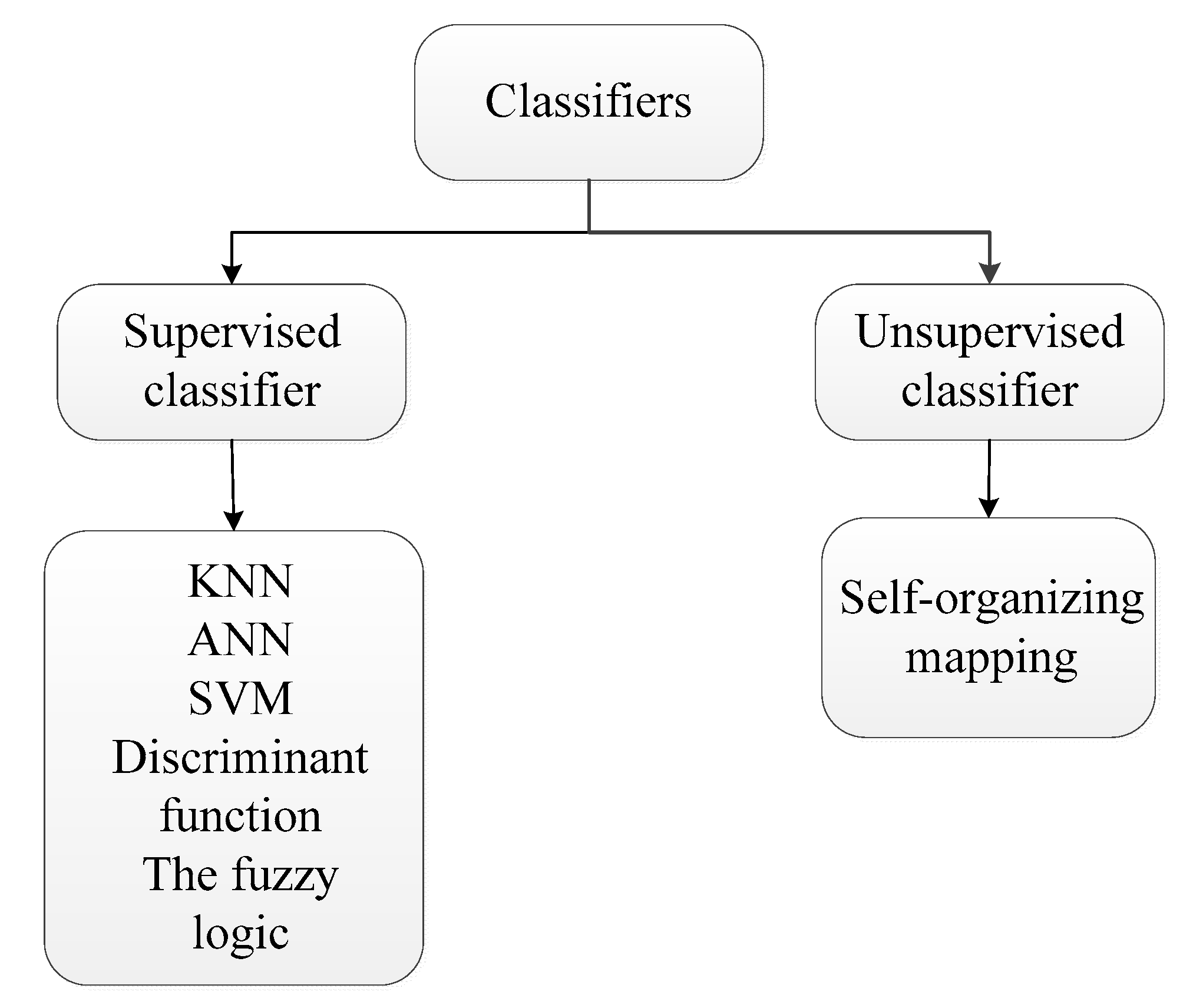
5. Classifier

The overall framework of the classifier is shown in Figure 8. There are two types of classifiers that are commonly used: supervised and unsupervised. The supervised classifier is a method of pattern recognition that is based on the samples provided by known training areas to find the characteristic parameters as decision rules, and then to establish the discriminant function to classify unknown sample images. The unsupervised classifier is an image classification method without a priori category standard, which is based on the characteristic differences of different image categories in the feature space. Based on the cluster theory, the decision rule of classification is established according to the statistical characteristics of the samples, and the classification is then presented.

5.1. Supervised Classifier

5.1.1. K-Nearest Neighbor (KNN)

The KNN method is uses the following steps. First, it extracts the characteristics of new data, and compares them with each data feature in the test set. Then, it extracts the nearest K data point’s feature labels from the test set. Finally, the most frequently occurring category of the nearest K data points is counted as the category of the new data.

The KNN algorithm is the simplest and most effective classification algorithm; it is simple and easy to implement. When the training data set is large, a large amount of storage space is required, and the distance between the samples to be measured and all of the samples in the training data set needs to be calculated, so it is very time-consuming, and time complexity is O(n) (which is a level of time complexity).

Ünsalan et al. [80] developed a texture analysis method combined with the K-nearest neighbor classifier to achieve satisfactory recognition accuracy; however, the method could not meet real-time requirements.

5.1.2. Artificial Neural Network

Artificial neural networks are free of the restrictions of early discrete transfer functions, and use continuous functions, such as sigmoid or hyperbolic tangent functions, to imitate the response of the neuron to excitation. The training process adopts the back propagation algorithm. The ANN resolves matters that could not be simulated or solved with logic problems before. Further, more layers allow the network to implement complex situations in practice. Moreover, this method can automatically construct nonlinear features, so it can be used to solve the problem of nonlinear partitions. Examples of practical applications include Martins [33], Wu [37], Kang [42], Tang [62], Li [68], Yazdchi [79], Yazdchi [86], among which Yazdchi [86] employed a three-layer feed forward neural network, with training by the error back-propagation method. Classification accuracy reached 97.89%. The publication of literatures using this classifier was mostly concentrated in 2000–2010, and its status in the mainstream has been gradually replaced since 2010.

5.1.3. Support Vector Machine

Since neural network training requires a large number of samples and there are multiple local optimums, the expression ability of shallow neural networks for feature learning is limited. However, there are many parameters in deep neural networks, which may lead to an overfitting problem. Support vector machines (SVMs) can overcome this problem. SVMs have the following advantages over neural networks (ANNs): (1) their cost function is convex, and there is a global optimal value; (2) they are able to cope with small sample sets; (3) they have good generalization performance and robustness; (4) the introduction of a kernel function solves the nonlinear problem; and, (5) they can also avoid the dimension disaster. In Neogi [87], Yu [32], Song [16], Chu [60], Wu [25], Liu [65], Jia [88], Zhao [36], Ghorai [26], Choi [43], Agarwal [29], the excellent performance of support vector machines is demonstrated. We found that there has been a large amount of literature based on support vector machine classifiers since 2010.

5.1.4. Discriminant Function (DF)

Pattern classification using discriminant functions not only depends on the geometric properties of the discriminant function (i.e., linear and nonlinear functions), it also depends on the coefficients of the discriminant function. As long as the samples that are being studied are separable, the coefficients of the discriminant function can be determined using a given set of samples [56,59].

5.1.5. Fuzzy Logic (FL)

Fuzzy logic based on the concept of a membership function makes use of fuzzy sets and fuzzy reasoning rules, and can represent transitional boundaries or qualitative knowledge experience. Therefore, fuzzy logic is good at expressing qualitative knowledge and experience with unclear boundaries. For example, an information extraction technique based on fuzzy logic and membership function theory to design decision rules is discussed in Blackledge [78].

5.1.6. Learning Vector Quantizer (LVQ)

The learning vector quantizer (LVQ) is a kind of supervised learning algorithm for pattern classification that was put forward in 1988, which is an extension of the unsupervised self-organizing map (SOM) algorithm. The basic idea of LVQ is to use a small number of weight vectors representing the topology of the data. Compared with the unsupervised self-organizing neural network algorithm, the LVQ algorithm has a wider application in the field of pattern recognition because of the introduction of supervised signals during the process of updating weight vectors. Olsson et al. [89] developed a statistical feature extraction technology combined with an LVQ classifier to complete defect inspection. Subsequently, Wu et al. [30] employed an FFT-based extraction feature combined with the LVQ classifier for the detection of surface defects in hot-rolled strips.

5.2. Unsupervised Classifier

The self-organizing map (SOM) is an important type of neural network based on unsupervised learning methods that was first put forward in 1981. Since then, with the rapid development of neural networks in the mid to late 1980s, self-organizing map theory and its applications have also made considerable progress. The self-organizing map network conducts classification by finding the optimal set of reference vectors. Compared with the traditional pattern clustering method, the clustering center can be mapped to a surface or a plane while keeping the topology unchanged. Hence, the problem of discriminating unknown cluster centers can be solved by using self-organizing maps. For example, in Kang [42], the authors researched an adaptive classification technique based on a combination of supervised learning neural network with error back-propagation (NN-BP) and unsupervised learning (SOM).

Table 7. Strengths and weaknesses of classifiers for steel defect recognition.

Name of Classifier		Strengths	Weaknesses
Supervised classifier	KNN	The algorithm is simple, clear, and easy to achieve.	Time consuming (time complexity is O(n)).
			Not suitable for the unbalanced distribution of samples.
	ANN	Suitable for nonlinear separable problems.	Too many layers (i.e., more than eight layers) make it prone to overfitting.
		High classification accuracy.
	SVM	Suitable for small sample sets.	Difficult to find the kernel function.
		Good generalization performance and robustness.
			Solving quadratic programming of functions requires a lot of storage space.
		Suitable for nonlinear problems.
		Suitable for high- dimensional situations.
	DF	Suitable for multi-class classification.	Difficult to determine the coefficients of functions.
		Accurate and efficient.
	FL	Suitable for expressing qualitative knowledge and experience in cases of unclear boundaries.	Poor classification accuracy (60%–85%).
	LVQ	Simple structure.	Input of heterogeneous samples will prevent convergence of weight vectors.
		Adaptive ability.	Information of each dimension of the input sample is not fully utilized.
Unsupervised classifier	SOM	Suitable for identifying unknown cluster centers.	“Dead nodes” can appear when the number of neuron nodes is more than the number of categories.
		Fault tolerant function.
		Self-associative function.

Note: KNN: K-nearest neighbor, ANN: Artificial neural network, SVM: Support vector machine, DF: Discriminant function, FL: Fuzzy logic, LVQ: Learning vector quantizer, SOM: Self-organizing map.

shows the performance comparison of classification methods for steel defects recognition.

6. Analysis

The following is an analysis of visual detection from the perspective of scientific literature to the perspective of market size.

6.1. Literature Analysis

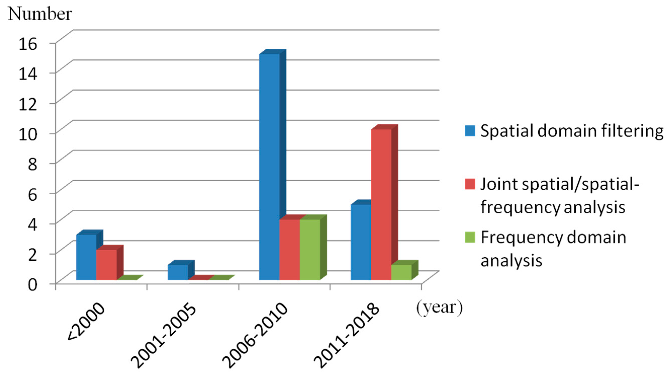
From the review of detection methods, we can see that a large number of publications over the past 30 years have been related to statistics and filtering methods, as shown in Figure 9.

From the point of development trends, both statistical methods and filtering methods have shown a significant downward trend since 2010, while the discussion of learning-based methods has steadily improved. This has much to do with the upsurge of deep learning in recent years. Model-based detection methods have always been out of the mainstream.

A detailed analysis of filtering methods is provided in Figure 10, because these methods have attracted much attention. From the 36 papers collected (relating to space filtering and frequency domains), it can be seen that although the best method of defect detection cannot be determined, it is clear that the joint spatial/frequency analysis methods (i.e., Gabor transform, wavelet transform, and MGA) have increased since 2010, which shows that these methods have been increasingly recognized by a majority of researchers.

In terms of classification methods, supervised classification methods have always dominated compared to unsupervised classification methods. As the knowledge set of defect models is imperfect, the supervised classification method is preferred if prior knowledge is available, since this method can achieve superior results.

Support vector machines and neural networks based on back propagation (NN-BP) are the mainstream supervised classification methods.

It can be seen from the Figure 11 that the NN-BP method was a classifier that was commonly discussed in the literature prior to 2010, and that the frequency of discussion of SVMs has increased sharply since 2010.

6.2. Market Size Analysis of Visual Inspection

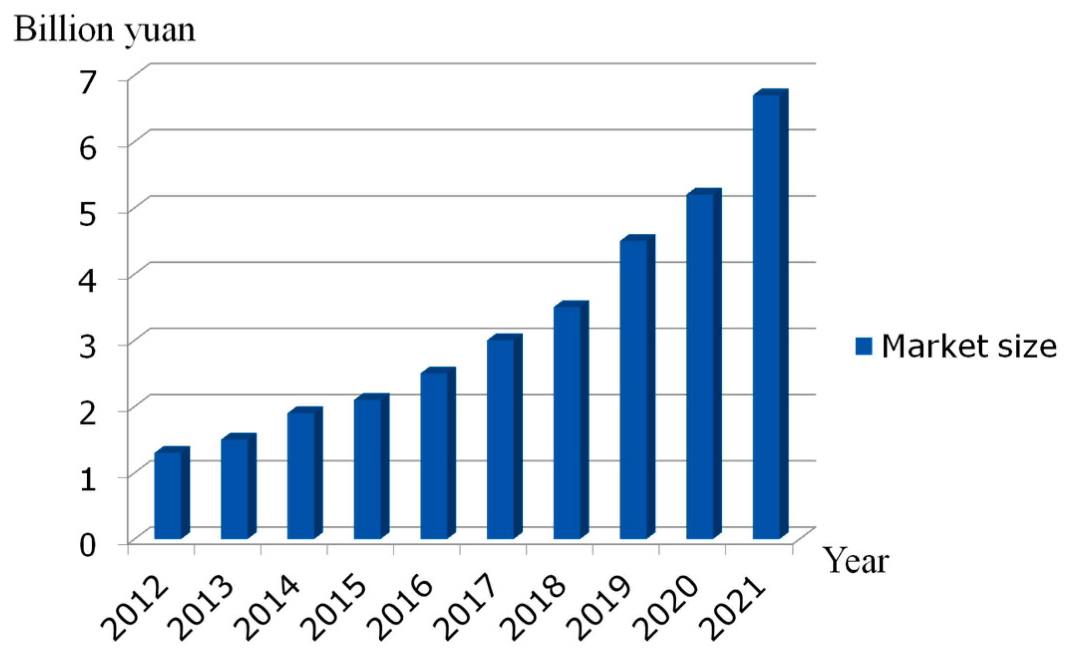
In 2017, the size of the global machine vision market was about USD $7.2 billion, growing 6.8% year-on-year. The market size is expected to be USD $7.7 billion in 2018, and could break through USD $9 billion in 2021, with an expected average annual compound growth rate of around 7.5% for 2018–2021. Germany and the United States are the world’s two largest national machine vision markets, accounting for more than 30% of the worldwide market in 2017. China’s machine vision industry has emerged since 2010, and is now in a period of rapid development. China’s market size in 2017 was CNY ¥2.9 billion (about USD $42.64 million), accounting for 6.41% of the global market, and up 18.3% year-on-year. With the deepening of automation and the intellectualization of various industries, it is estimated that the average annual growth rate of China’s machine vision market will be around 20% in 2018–2021, which was higher than the global average growth rate, as shown in Figure 12 [90].

The world’s major machine vision manufacturers include Keenshi, Konrad, Darsa, Panasonic, and Omron. In 2016, their combined market share was about 38.0%. Typical Chinese enterprises are Daheng, New Epoch Technology, and Shenzhen JT Automation Equipment, which are less competitive compared with international well-known players, and each made up less than 1.5% of the global market in 2016.

At present, Chinese machine vision products are mainly used in semiconductor, electronic manufacturing, automobile, and other fields. The demand for machine vision in these fields accounted for nearly 60% of total demand in 2017.

7. Conclusions

In this paper, studies of software and hardware for visual detection from 90 papers are reviewed. The discussion of hardware includes coverage of cameras, light sources, and lighting modes, and a basis of selection is provided. In the software discussion, detection methods are divided into the categories of statistics, filtering, models, and machine learning according to basic theories of image processing. Classification methods are divided into supervised and unsupervised learning. The main ideas, advantages, and disadvantages of these methods are discussed, which can help users choose the most appropriate methods for different application environments.

Recommendations relating to the key technologies of visual detection, cameras, light sources, and image-processing algorithms can be summarized as follows:

• The linear array camera is an inevitable choice for the selection of industrial cameras, because area-array cameras cannot achieve the resolution and frame rate required in conditions of high detection accuracy and fast motion. The frame rate of the camera must be greater than the speed of the object. Therefore, large frame rate, small pixel size line array cameras have good development prospects.
• LED light sources have good color performance, a wide spectrum range (i.e., they can cover the whole range of visible light), high luminous intensity, and a long period of stability. As their manufacturing processes and technology matures, and prices fall, LED lamps will be used more widely.
• It is difficult to select one kind of detection algorithm to meet the range of needs of accurate detection for multiple types of unbalanced defects; therefore, the fusion of multiple technologies is an expected trend.
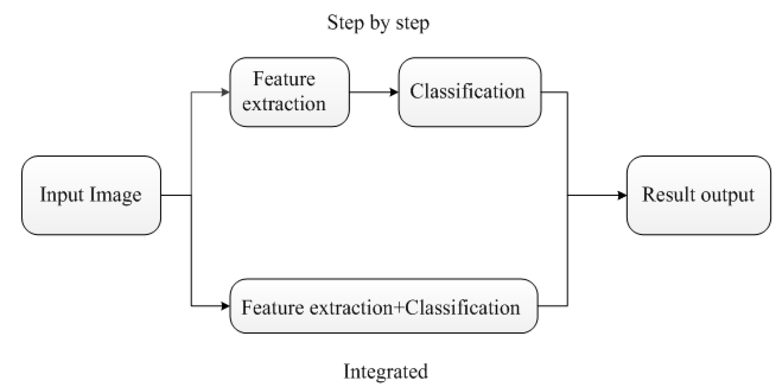
• The conventional detection process starts with feature extraction, followed by classification and a result output. The feature extraction process adopts artificial design features, and is tedious and complicated. However, the end-to-end approach combines feature extraction and the classification process into one body through deep learning neural networks, and features are extracted automatically through the learning of training sets (Figure 13), as seen in Yi [40], Park [82], Masci [21]. This method is simple and achieves high detection accuracy. Moreover, it can be readily generalized. However, its biggest disadvantage is that it needs a large number of training images, with specific needs of training sets (e.g., the training set must cover sufficient defect types); otherwise, detection results are not ideal. The excellent performance of convolutional networks based on deep learning in the field of image processing makes it inevitable that it will be developed further in the future. The convolutional neural network algorithm with small and zero samples will be the focus of future research in the field of visual detection.
• For industrial applications, it is important that real-time performance meets production requirements. However, detection accuracy depends on the complexity of the deep network, while the complexity of the network can restrict the production process. Therefore, it is a direction of future efforts to find a balance between algorithm complexity, detection accuracy, and time taken for detection.
• A well-recognized standard data set and a good communication protocol for experimental data is required for the detection of defects on steel surfaces. Only in this way can fair, comparative analysis be realized.

In addition, our future work will pay attention to research progress on the detection of surface defects of steel products based on image processing in order to continuously enrich and update the relevant literature review.

References

- Pinho, E.; Costa, C. Unsupervised learning for concept detection in medical images: A comparative analysis. Appl. Sci. 2018, 8, 1213. [Google Scholar] [CrossRef]
- Kong, X.; Li, J. Image Registration-Based Bolt Loosening Detection of Steel Joints. Sensors 2018, 18, 1000. [Google Scholar] [CrossRef] [PubMed]
- Kong, X.; Li, J. Vision-Based Fatigue Crack Detection of Steel Structures Using Video Feature Tracking. Comput.-Aided Civ. Inf. 2018, 9, SI783–SI799. [Google Scholar] [CrossRef]
- Calvo-Zaragoza, J.; Castellanos, F.J.; Vigliensoni, G.; Fujinaga, I. Deep neural networks for document processing of music score images. Appl. Sci. 2018, 8, 654. [Google Scholar]
- Cho, C.S.; Chung, B.M.; Park, M.J. Development of real-time vision-based fabric inspection system. IEEE Trans. Ind. Electron. 2005, 52, 1073–1079. [Google Scholar] [CrossRef]
- Gao, X.; Wu, Y.; Yang, K. Vehicle bottom anomaly detection algorithm based on sift. Optik 2015, 126, 3562–3566. [Google Scholar]
- Jang, T.S.; Lee, S.S.; Kwon, I.B.; Lee, W.J.; Lee, J.J. Noncontact detection of ultrasonic waves using fiber optic sagnac interferometer. IEEE Trans. Ultrason. Ferroelectr. Frequency Control 2002, 49, 767–775. [Google Scholar] [CrossRef]
- Chin, R.T.; Harlow, C.A. Automated visual inspection: A survey. IEEE Trans. Pattern Anal. Mach. Intell. 1982, 4, 557–573. [Google Scholar] [CrossRef] [PubMed]
- Newman, T.S.; Jain, A.K. A survey of automated visual inspection. Vis. Image Underst. 1995, 61, 231–262. [Google Scholar] [CrossRef]
- Li, Y.; Gu, P. Free-form surface inspection techniques state of the art review. Comput. Aided Des. 2004, 36, 1395–1417. [Google Scholar]
- Shirvaikar, M. Trends in automated visual inspection. J. Real-Time Image Process. 2006, 1, 41–43. [Google Scholar] [CrossRef]
- Hanbay, K.; Talu, M.F.; Özgüven, Ö.F. Fabric defect detection systems and methods—A systematic literature review. Optik 2016, 127, 11960–11973. [Google Scholar] [CrossRef]
- Jfs, G.; Leta, F.R. Applications of computer vision techniques in the agriculture and food industry: A review. Eur. Food Res. Technol. 2012, 235, 989–1000. [Google Scholar]
- Eui Jae, R.I. Dependences of the reflectivity and adhesion of thin metal films on the various process parameters for polyester substrates during physical vapor depositions. Met. Mater. Int. 2002, 8, 591–599. [Google Scholar]
- Neogi, N.; Mohanta, D.K.; Dutta, P.K. Review of vision-based steel surface inspection systems. EURASIP J. Image Video Process. 2014, 1, 50. [Google Scholar] [CrossRef]
- Song, K.; Yan, Y. A noise robust method based on completed local binary patterns for hot-rolled steel strip surface defects. Appl. Surf. Sci. 2013, 285, 858–864. [Google Scholar] [CrossRef]
- Yun, J.P.; Choi, S.H.; Jeon, Y.; Choi, D.; Kim, S.W. Detection of line defects in steel billets using undecimated wavelet transform. In Proceedings of the 2008 IEEE International Conference on Control, Automation and Systems, Seoul, Korea, 14–17 October 2008; pp. 1725–1728. [Google Scholar]
- Dupont, F.; Odet, C.; Cartont, M. Optimization of the recognition of defects in flat steel products with the cost matrices theory. NDT E Int. 1997, 30, 3–10. [Google Scholar] [CrossRef]
- Yun, J.P.; Choi, S.H.; Seo, B.; Chang, H.P.; Sang, W.K. Defects detection of billet surface using optimized gabor filters. IFAC Proc. Vol. 2008, 41, 77–82. [Google Scholar] [CrossRef]
- Ai, Y.H.; Xu, K. Surface Detection of Continuous Casting Slabs Based on Curvelet Transform and Kernel Locality Preserving Projections. J. Iron. Steel Res. Int. 2013, 20, 80–86. [Google Scholar] [CrossRef]
- Masci, J.; Meier, U.; Ciresan, D.; Schmidhuber, J. Steel defect classification with Max-Pooling Convolutional Neural Networks. International Joint Conference on Neural Networks, Brisbane, QLD, Australia, 10–15 June 2012; IEEE: Piscataway, NJ, USA, 2012; Volume 20, pp. 1–6. [Google Scholar]
- Luo, Q.; He, Y. A cost-effective and automatic surface defect inspection system for hot-rolled flat steel. Robot. Cim.-Int. Manuf. 2016, 38, 16–30. [Google Scholar] [CrossRef]
- Liu, M.; Liu, Y.; Hu, H.; Nie, L. Genetic algorithm and mathematical morphology based binarization method for strip steel defect image with non-uniform illumination. J. Vis. Commun. Image Represent. 2016, 37, 70–77. [Google Scholar] [CrossRef]
- Wu, X.; Xu, K.; Xu, J. Application of Undecimated Wavelet Transform to Surface Defect Detection of Hot Rolled Steel Plates. In Proceedings of the 2008 IEEE Conference on Image and Signal, Sanya, China, 27–30 May 2008; pp. 528–532. [Google Scholar]
- Wu, G.; Kwak, H.; Jang, S.; Xu, K.; Xu, J. Design of online surface inspection system of hot rolled strips. In Proceedings of the 2008 IEEE International Conference on Automation and Logistics, Qingdao, China, 1–3 September 2008; pp. 2291–2295. [Google Scholar]
- Ghorai, S.; Mukherjee, A.; Gangadaran, M. Automatic defect detection on hot-rolled flat steel products. IEEE Trans. Instrum. Meas. 2013, 62, 612–621. [Google Scholar] [CrossRef]
- Zhang, X. Image Fusion Method for Strip Steel Surface Detect Based on Bandelet-PCNN. Adv. Mater. Res. 2012, 546–547, 806–810. [Google Scholar] [CrossRef]
- Caleb, P.; Steuer, M. Classification of surface defects on hot rolled steel using adaptive learning methods. In Proceedings of the International Conference on Knowledge-Based Intelligent Engineering Systems and Allied Technologies, Brighton, UK, 30 August–1 September 2000; IEEE: Piscataway, NJ, USA, 2000; pp. 103–108. [Google Scholar]
- Agarwal, K.; Shivpuri, R.; Zhu, Y.; Chang, T.S.; Huang, H. Process knowledge based multi-class support vector classification (PK-MSVM) approach for surface defects in hot rolling. Expert. Syst. Appl. 2011, 38, 7251–7262. [Google Scholar] [CrossRef]
- Wu, G.; Zhang, H.; Sun, X. A Bran-new Feature Extraction Method and its application to Surface Defect Recognition of Hot Rolled Strips. In Proceedings of the IEEE International Conference on Automation and Logistics, Jinan, China, 18–21 August 2007; pp. 2069–2074. [Google Scholar]
- Liu, W.; Yan, Y. Automated surface defect detection for cold-rolled steel strip based on wavelet anisotropic diffusion method. Int. J. Ind. Syst. Eng. 2014, 17, 224–239. [Google Scholar] [CrossRef]
- Yu, Y.W.; Yin, G.F.; Du, L.Q. Image classification for steel strip surface defects based on support vector machines. Adv. Mater. Res. 2011, 217–218, 336–340. [Google Scholar] [CrossRef]
- Martins, L.A.O.; PaáDua, F.L.C.; Almeida, P.E.M. Automatic detection of surface defects on rolled steel using Computer Vision and Artificial Neural Networks. In Proceedings of the IECON 2010—36th Annual Conference on IEEE Industrial Electronics Society, Glendale, AZ, USA, 7–10 Novrmber 2010; pp. 1081–1086. [Google Scholar]
- Toshihiro, S.; Hideki, T.; Yasuo, T. Automatic surface inspection system for tin mill black plate (TMBP). JFE Tech. Rep. 2007, 9, 60–63. [Google Scholar]
- Yun, S.W.; Kong, N.W.; Lee, G.; Park, P.G. Development of defect detection algorithm in cold rolling. Int. J. Control Autom. 2008, 1, 1729–1733. [Google Scholar]
- Zhao, J.; Zhao, J.; Yang, Y.; Li, G. The Cold Rolling Strip Surface Defect On-Line Inspection System Based on Machine Vision. In Proceedings of the Second Pacific-Asia Conference on IEEE Circuits, Communications and System (PACCS), Beijing, China, 1–2 August 2010; pp. 402–405. [Google Scholar]
- Wu, G.F. Online Surface Inspection Technology of Cold Rolled Strips, Multimedia; InTech: London, UK, 2010. [Google Scholar]
- Wu, G.; Xu, K.; Xu, J. Application of a new feature extraction and optimization method to surface defect recognition of cold rolled strips. Int. J. Min. Met. Mater. 2007, 14, 437–442. [Google Scholar] [CrossRef]
- Peng, K.; Zhang, X. Classification Technology for Automatic Surface Defects Detection of Steel Strip Based on Improved BP Algorithm. In Proceedings of the International Conference on Natural Computation IEEE, Tianjin, China, 14–16 August 2009; Volume 1, pp. 110–114. [Google Scholar]
- Yi, L.; Li, G.; Jiang, M. An End-to-End Steel Strip Surface Defects Recognition System Based on Convolutional Neural Networks. Steel Res. Int. 2016, 88, 176–187. [Google Scholar] [CrossRef]
- Masci, J.; Meier, U.; Fricout, G.; Schmidhuber, J. Multi-scale pyramidal pooling network for generic steel defect classification. In Proceedings of the International Joint Conference on Neural Networks, Dallas, TX, USA, 4–9 August 2013; Piscataway, NJ, USA, 2014; pp. 1–8. [Google Scholar]
- Kang, G.W.; Liu, H.B. Surface defects inspection of cold rolled strips based on neural network. In Proceedings of the International Conference on Machine Learning and Cybernetics IEEE, Guangzhou, China, 18–21 August 2005; Volume 8, pp. 5034–5037. [Google Scholar]
- Choi, K.; Koo, K.; Jin, S.L. Development of Defect Classification Algorithm for POSCO Rolling Strip Surface Inspection System. In Proceedings of the International Joint Conference IEEE, SICE-ICASE, Busan, Korea, 18–21 October 2006; Volume 2007, pp. 2499–2502. [Google Scholar]
- Kaya, K.; Bilgutay, N.M.; Murthy, R. Flaw detection in stainless steel samples using wavelet decomposition. In Proceedings of the 1994 IEEE Conference on Ultrasonics Symposium, Cannes, France, 31 October–3 November 1994; pp. 1271–1274. [Google Scholar]
- Choi, S.H.; Yun, J.P.; Seo, B.; Sang, W.K. Real-time defects detection algorithm for high-speed steel bar in coil, world academy of science. Eng. Technol. 2007, 25, 66–70. [Google Scholar]
- Bulnes, F.G.; Usamentiaga, R.; García, D.F.; Molleda, J. Vision-based sensor for early detection of periodical defects in web materials. Sensors 2012, 12, 10788–10809. [Google Scholar] [CrossRef] [PubMed]
- Li, W.B.; Lu, C.H.; Zhang, J.C. A local annular contrast based real-time inspection algorithm for steel bar surface defects. Appl. Surf. Sci. 2012, 258, 6080–6086. [Google Scholar] [CrossRef]
- Zhang, J.; Kang, D.; Won, S. Detection of scratch defects for wire rod in steelmaking process. In Proceedings of the 2010 IEEE International Conference on Control, Automation and Systems, Gyeonggi-do, Korea, 27–30 October 2010; pp. 319–323. [Google Scholar]
- Yun, J.P.; Choi, D.C.; Jeon, Y.J. Defect inspection system for steel wire rods produced by hot rolling process. Int. J. Adv. Manuf. Technol. 2014, 70, 1625–1634. [Google Scholar] [CrossRef]
- Choi, D.C.; Jeon, Y.J.; Lee, S.J.; Yun, J.P.; Kim, S.W. Algorithm for detecting seam cracks in steel plates using a gabor filter combination method. Appl. Opt. 2014, 53, 4865–4872. [Google Scholar] [CrossRef] [PubMed]
- Koller, N.; O’Leary, P.; Lee, P. Comparison of cmos and ccd cameras for laser profiling. In Proceedings of the SPIE the International Society for Optical Engineering, San Jose, CA, USA, 3 May 2004; pp. 108–115. [Google Scholar]
- Lee, S.H.; Yang, C.S. A real time object recognition and counting system for smart industrial camera sensor. IEEE Sens. J. 2017, 17, 2516–2523. [Google Scholar] [CrossRef]
- Nguyen, A.Q.; Vts, D.; Shimonomura, K.; Takehara, K.; Etoh, T.G. Toward the ultimate-high-speed image sensor: From 10 ns to 50 ps. Sensors 2018, 18, 2407. [Google Scholar] [CrossRef] [PubMed]
- Wu, L.; Zhu, J.; Xie, H. A modified virtual point model of the 3d dic technique using a single camera and a bi-prism. Meas. Sci. Technol. 2014, 25, 115008. [Google Scholar] [CrossRef]
- Zheng, H.; Kong, L.X.; Nahavandi, S. Automatic inspection of metallic surface defects using genetic algorithms. J. Mater. Process. Technol. 2002, 125, 427–433. [Google Scholar] [CrossRef] [Green Version]
- Cord, A.; Bach, F.; Jeulin, D. Texture classification by statistical learning from morphological image processing: Application to metallic surfaces. J. Microsc. 2010, 239, 159–166. [Google Scholar] [CrossRef] [PubMed]
- Yun, J.P.; Park, C.; Bae, H.; Hwang, H.; Choi, S. Vertical Scratch Detection Algorithm for High-speed Scale-covered Steel BIC (Bar in Coil). In Proceedings of the 2010 IEEE International Conference on Control Automation and Systems, Gyeonggi-do, Korea, 27–30 October 2010; Volume 6245, pp. 342–345. [Google Scholar]
- Haralick, R.M. Statistical and structural approaches to texture. Proc. IEEE 2005, 67, 786–804. [Google Scholar] [CrossRef]
- Liu, W.; Yan, Y.; Li, J.; Zhang, Y.; Sun, H. Automated On-Line Fast Detection for Surface Defect of Steel Strip Based on Multivariate Discriminant Function. In Proceedings of the 2008 IEEE Second International Symposium on Intelligent Information Technology Application, Computer Society, Shanghai, China, 20–22 December 2008; Volume 2, pp. 493–497. [Google Scholar]
- Chu, M.; Gong, R.; Gao, S.; Zhao, J. Steel surface defects recognition based on multi-type statistical features and enhanced twin support vector machine. Chemometr. Intell. Lab. 2017, 171, 140–150. [Google Scholar] [CrossRef]
- Guo, J.H.; Meng, X.D.; Xiong, M.D. Study on Defection Segmentation for Steel Surface Image Based on Image Edge Detection and Fisher Discriminant. J. Phys. Conf. Ser. 2006, 48, 364–368. [Google Scholar] [CrossRef] [Green Version]
- Tang, B.; Kong, J.Y.; Wang, X.D.; Chen, L. Surface Inspection System of Steel Strip Based on Machine Vision. In Proceedings of the First International Workshop on Database Technology and Applications, Wuhan, China, 25–26 April 2009; pp. 359–362. [Google Scholar]
- Yang, S.S.; He, Y.H.; Wang, Z.L.; Zhao, W.S. A method of steel strip image segmentation based on local gray information. In Proceedings of the 2008 IEEE International Conference on Industrial Technology, Chengdu, China, 21–24 April 2008; pp. 1–4. [Google Scholar]
- Guan, S. Strip Steel Defect Detection Based on Saliency Map Construction Using Gaussian Pyramid Decomposition. ISIJ Int. 2015, 55, 1950–1955. [Google Scholar] [CrossRef] [Green Version]
- Liu, Y.C.; Hsu, Y.L.; Sun, Y.N.; Tsai, S.J.; Ho, C.Y.; Chen, C.M. A computer vision system for automatic steel surface inspection. In Proceedings of the fifth IEEE conference on Industrial Electronics and Applications (ICIEA), Taichung, Taiwan, 15–17 June 2010; pp. 1667–1670. [Google Scholar]
- Jeon, Y.J.; Choi, S.H.; Yun, J.P. Detection of scratch defects on slab surface. In Proceedings of the 1994 IEEE International Conference on Control, Automation and Systems, Gyeonggi-do, Korea, 26–29 October 2011; pp. 1274–1278. [Google Scholar]
- Choi, D.; Yun, J.P.; Sang, W.K.; Jeon, Y. Pinhole detection in steel slab images using gabor filter and morphological features. Appl. Opt. 2011, 50, 5122–5129. [Google Scholar] [CrossRef] [PubMed]
- Li, J.; Shi, J.; Chang, T.S. On-line seam detection in rolling processes using snake projection and discrete wavelet transform. J. Manuf. Sci.-Trans. ASME 2006, 129, 926–933. [Google Scholar] [CrossRef]
- Xu, S.H.; Guan, S.Q.; Chen, L.L. Steel Strip Defect Detection based on Human Visual Attention Mechanism Model. Appl. Mech. Mater. 2014, 530–531, 456–462. [Google Scholar] [CrossRef]
- Candès, E.J.; Donoho, D.L. Ridgelets: A key to higher-dimensional intermittency? Philos. Trans. Math. Phys. Eng. Sci. 1999, 357, 2495–2509. [Google Scholar]
- Claypoole, R.L., Jr.; Baraniuk, R.G. Multiresolution wedgelet transform for image processing. In Proceedings of the SPIE—The International Society for Optical Engineering, San Diego, CA, USA, 4 December 2000; Volume 4119, pp. 253–262. [Google Scholar]
- Donoho, D.L.; Huo, X. Beamlets and Multiscale Image Analysis. Multiscale Multiresolut. Methods 2001, 20, 149–196. [Google Scholar]
- Candès, E.J.; Donoho, D.L. Recovering edges in ill-posed inverse problems: Optimality of curvelet frames. Ann. Stat. 2002, 30, 784–842. [Google Scholar] [CrossRef]
- Pennec, E.L.; Mallat, S. Bandelet representations for image compression. In Proceedings of the 2001 IEEE International Conference on Image Processing, Thessaloniki, Greece, 7–10 October 2001; p. 12. [Google Scholar]
- Do, M.N.; Vetterli, M. Contourlets: A Directional Mulitresolution Image Representation. In Proceedings of the 1994 IEEE International Conference on Image Processing, Rochester, NY, USA, 22–25 September 2002; pp. 357–360. [Google Scholar]
- Xu, K.; Xu, Y.; Zhou, P.; Wang, L. Application of RNAMlet to surface defect identification of steels. Opt. Laser Eng. 2018, 105, 110–117. [Google Scholar] [CrossRef]
- Mandelbrot, B.B. The Fractal Geometry of Nature; W. H. Freeman: New York, NY, USA, 1983. [Google Scholar]
- Blackledge, J.; Dubovitskiy, D. A Surface Inspection Machine Vision System that Includes Fractal Texture Analysis. Dublin Inst. Technol. 2008, 3, 76–89. [Google Scholar]
- Yazdchi, M.; Yazdi, M.; Mahyari, A.G. Steel Surface Defect Detection Using Texture Segmentation Based on Multifractal Dimension. In Proceedings of the International Conference on Digital Image Processing, Bangkok, Thailand, 7–9 March 2009; pp. 346–350. [Google Scholar]
- Ünsalan, C.; Erçil, A. Automated Inspection of Steel Structures, Recent Advances in Mechatronics; Springer Ltd.: Singapore, 1999. [Google Scholar]
- Zhao, X.Y.; Lai, K.S.; Dai, D.M. An improved bp algorithm and its application in classification of surface defects of steel plate. J. Iron Steel Res. (Int.) 2007, 14, 52–55. [Google Scholar] [CrossRef]
- Park, J.K.; Kwon, B.K.; Park, J.H.; Kang, D.J. Machine learning-based imaging system for surface defect inspection. Int. J. Precis. Eng. Manuf. Green Technol. 2016, 3, 303–310. [Google Scholar] [CrossRef]
- Chu, M.; Zhao, J.; Liu, X.; Gong, R. Multi-class classification for steel surface defects based on machine learning with quantile hyper-spheres. Chemometr. Intell. Lab. 2017, 168, 15–27. [Google Scholar] [CrossRef]
- Gong, R.; Wu, C.; Chu, M. Steel surface defect classification using multiple hyper-spheres support vector machine with additional information. Chemometr. Intell. Lab. 2018, 172, 109–117. [Google Scholar] [CrossRef]
- Liu, Z.; Hu, J.; Hu, L.; Zhang, X.L.; Kong, J.Y. Research on on-line surface defect detection for steel strip based on sparse coding. Adv. Mater. Res. 2012, 548, 749–752. [Google Scholar] [CrossRef]
- Yazdchi, M.R.; Mahyari, A.G.; Nazeri, A. Detection and Classification of Surface Defects of Cold Rolling Mill Steel Using Morphology and Neural Network. In Proceedings of the 2008 IEEE International Conference on Computational Intelligence for Modelling Control & Automation, Vienna, Austria, 24 July 2009; pp. 1071–1076. [Google Scholar]
- Neogi, N.; Mohanta, D.K.; Dutta, P.K. Defect detection of steel surfaces with global adaptive percentile thresholding of gradient image. J. Inst. Eng. 2017, 98, 557–565. [Google Scholar] [CrossRef]
- Jia, H.; Yi, L.M.; Shi, J.; Chang, T.S. An Intelligent Real-time Vision System for Surface Defect Detection. In Proceedings of the International Conference on Pattern Recognition IEEE, Cambridge, UK, 26 August 2004; pp. 239–242. [Google Scholar]
- Olsson, J.; Gruber, S. Web process inspection using neural classification of scattering light. IEEE Trans. Ind. Electron. 1993, 40, 228–234. [Google Scholar] [CrossRef]
- Global and China Machine Vision Industry Report. Available online: http://www.pday.com.cn/Htmls/Report/201704/24516162.html (accessed on 24 April 2017).
Figure 1.
Visual inspection system. Note: CCD: Charge coupled devices; ROI: Region of interest.
Figure 2.
Types of steel products (reproduced from Neogi [15]).
Figure 3.
Examples of steel defects (reproduced from Song [16]).
Figure 4.
(a) Stroboscopic xenon lamps; (b) Halogen lamps; (c) Light-emitting diode (LED) lamps.
Figure 5.
Lighting methods.
Figure 6.
Classification map of steel surface defect detection methods.
Figure 7.
Artificial neural networks (ANN) model.
Figure 8.
Kinds of classifiers. Note. KNN: K-nearest neighbor, ANN: artificial neural network, SVM: support vector machine.
Figure 9.
Distribution map detection method.
Figure 10.
Distribution of filtering detection methods.
Figure 11.
Distribution of classification methods.
Figure 12.
China machine vision market size.
Figure 13.
Two models of image processing.