Failure Identification of Dump Truck Suspension Based on an Average Correlation Stochastic Subspace Identification Algorithm

Abstract

This paper proposes a fault identification method based on an improved stochastic subspace modal identification algorithm to achieve high-performance fault identification of dump truck suspension. The sensitivity of modal parameters to suspension faults is evaluated, and a fault diagnosis method based on modal energy difference is established. The feasibility of the proposed method is validated by numerical simulation and full-scale vehicle tests. The result shows that the proposed average correlation signal based stochastic subspace identification (ACS-SSI) method can identify the fluctuation of vehicle modal parameters effectively with respect to different spring stiffness and damping ratio conditions, and then fault identification of the suspension system can be realized by the variation of the modal energy difference (MED).

1. Introduction

The suspension system is the component of a vehicle that connects the vehicle body and the wheel, which supports the car body and isolates the shock and vibration caused by road unevenness [1]. The suspension system is crucial for vehicle safety and riding comfort, and also plays an important role in handling and braking. Due to a poor working environment and complex operating conditions, failures often occur during in dump truck suspension systems in operation, which have a huge impact on the efficiency and reliability of fleet operations, and also endanger property and driver safety [2].

Therefore, methods for condition monitoring of the vehicle suspension system have attracted much attention [3,4,5,6]. There are two main types of fault diagnosis algorithms: data-driven methods and model-based methods. If the diagnosis process does not require a physical model and instead depends on measured data, it is referred to as a data-driven fault diagnosis method [7]; for example, independent component analysis (ICA), and principle component analysis (PCA). Furthermore, many methods are published to be applied in the fault diagnosis of suspension systems. He et al. combine k-means clustering with Fisher discriminant analysis (FDA) to conduct fault diagnoses of suspension systems [8]. Likewise, canonical vitiate analysis (CVA) and dynamical principle components analysis (DPCA) are applied to detect early faults [9]. Moreover, adaptive fuzzy c-means (FCM) clustering has been developed for condition monitoring, and possibilistic c-means (PCM) clustering with fault lines have been designed to isolate the faults [10,11].

Data-driven fault diagnosis methods have the advantage of not requiring a numerical model. However, these models are susceptible to noise and varied operation conditions. Unfortunately, because of the poor working environment and complex operation conditions, the noise is strong and excitation from the road is intensive and varied, so data-driven methods have not been well suited to the failure identification of dump truck suspension to date.

By contrast, in model-based fault diagnosis methods, a precise model is needed to be built [12,13,14,15,16,17]. Several model-based fault diagnosis methods are implemented in research; a Kalman-filter based fault diagnosis method with high efficiency has been developed [18], and a distributed-observer based fault detection and an interaction multi-model approach are proposed respectively for the damper and spring [19,20]. However, the difficulty makes it hard to obtain the parameters of a dynamic system for modeling.

Identification of modal parameters is an approach to obtain the dynamic characteristic of a system [21,22], and it can acquire accurate dynamic parameters via test signals, such as subspace identification (SI) [23,24]. Moaveni et al. [25] used deterministic subspace identification (DSI) to identify the modal parameters of nonlinear systems, and proposed a method of determining the nonlinear dynamic characteristics based on the identification of deterministic subspace and time-varying modal parameters. Moreover, the output-only identification methods can recognize the mode using the response only [26]. Sarmadi et al. [27] proposed a recursive adaptive stochastic subspace method to monitor the modes of the dynamic system online using wide-area synchronous vector data. Chen et al. [28,29] used the average correlated stochastic subspace method (ASC-SSI) to identify the operating modal of the frame online, obtained the frame modal parameters under constraint conditions, and matched the relevant components according to the identification result. Dong et al. [30] used the stochastic subspace method to identify vehicle modal parameters and calculate the variation in vehicle inertia parameters. This study illustrates that the noise and high damping ratio (20–30%) greatly influences the identification results of the stochastic subspace method.

This paper puts forward an online monitoring and diagnosis method for early faults of truck suspension systems. The average correlation signal based stochastic subspace identification (ACS-SSI) is adopted because of its advantages, including the low testing hardware requirements, high identification accuracy, and suitability for random vibration conditions. However, the challenge is dealing with the impact of noise and high damping ratios, so the vehicle vibration model with 11 degrees of freedom (DOFs) is established to verify the performance under different signal-to-noise ratios (SNR) and damper damping ratios, and then the modal parameters of the vehicle are identified by both numerical simulation and experiments. Moreover, the sensitivity of each modal parameter is evaluated, and a fault diagnosis method based on the modal energy difference method is established. Finally, the feasibility of the developed fault diagnosis method is validated by experimental tests carried out on a full-scale vehicle.

The rest of this paper is organized as follows. Section 2 introduces the principles of ACS-SSI briefly, and verifies its robustness under noise and high damping ratios. Section 3 proposes the failure identification method and builds the 11 DOF model to simulate the diagnosis process. Section 4 conducts the real-scale experiment. Finally, the paper ends with conclusions in Section 5.

2. ACS-SSI Algorithm and Its Verification

Considering the advantages and disadvantages of covariance-driven stochastic subspace identification (COV-SSI), this paper improves the covariance-driven subspace method using the noise suppression characteristics of the average correlation function. The use of multiple average correlation functions to replace the original vibration signal as the input can theoretically reduce the influence of noise signals on the identification accuracy. Therefore, the average correlation signal based stochastic subspace identification (ACS-SSI) is applied to the identification of modal characteristics of dynamic systems. The effectiveness of the improved method is initially verified based on a multi-DOF dynamic model.

2.1. Basic Principle of ACS-SSI

Stochastic subspace identification (SSI) can achieve modal identification only with output signals relying on the system input data. The process can be summarized as follows. First, the control matrix and the observable matrix are obtained by the singular value decomposition of the covariance of the response data; then, the modal parameters of the state matrix can be derived [29]. The kinematic equations can be written as the discrete-state space stochastic equation

$$\{\begin{array}{l}x(k+1)=Ax(k)+w(k)\\ y(k+1)=Cx(k)+v(k)\end{array},$$

(1)

where A is the state space matrix, C is the output space matrix, w(k) is the representative random input signal which includes the process noise, v(k) is the measurement of noise and k is the discrete time value. The state space matrix A contains the modal information of the system.

The state matrix A is reconstructed by the stochastic subspace method and the modal parameters can be extracted from it. The matrix of l-channel measurement signals collected by l channels is y(t), in which the one with a better signal-to-noise ratio (SNR) is chosen and set as the k-th signal y_k(t). The correlation function of all the original signals for the k-th channel is:

$$r_k(\tau )=\frac{1}{n}[y(t+\tau )\cdot y_k(t)],$$

(2)

where τ = 1, 2,…, N − n is the discrete time series of the correlation function, with N being the total length of the collected signal. The correlation function $r_k(\tau )\in R^{l*\tau }$ is an l-way signal related to a set of τ correlation functions. In order to improve the denoising effect, a multi-group experiment was carried out to obtain the n-group signal r_k1, r_k2, …, r_kn; the n-group signal was averaged to obtain an average correlation function $\overline{r_k(\tau )}$ used to replace the original y(t) as the input for modal identification.

The subsequent steps are the same as the covariance-driven stochastic subspace method [26]: using the covariance of $\overline{r_k(\tau )}$ to form the matrix $T_{1/i}$, the singular value decomposition (SVD) is carried out to obtain the discrete state matrix A. After decomposing matrix A, the eigenvalue ${\lambda }_i$ and eigenvector ${\Psi }_i$ are obtained and then converted into natural frequency f_ni, modal damping ratio ξ_i, and modal vector v_i.

2.2. Numerical Simulation in Multi-DOF System

2.2.1. Multi-DOF Numerical Simulation

A three-DOFs numerical simulation model is established in Matlab/Simulink software to verify the robustness of the improved stochastic subspace algorithm and its reliability for high damping ratios (Figure 1). The mass blocks m₁, m₂, m₃ are connected by the fixed stiffness k₁, k₂, k₃ and damping c₁, c₂, c₃, respectively. The three natural frequencies of the system f_n1 = 2.5 Hz, f_n2 = 5.8 Hz, f_n3 = 9.9 Hz, are determined by both mass and stiffness. Three low-pass filtered white noise signals, w₁, w₂, and w₃, are applied to the three mass units to simulate dynamic behaviors under random excitation.

The sampling frequency of the simulation system is 200 Hz, the solution time is 20 s, and the average correlation calculation is carried out 50 times. The dynamic responses of the vehicle suspension are concentrated primarily in the frequency range of 0–50 Hz [31]. Therefore, according to the Nyquist sampling theorem, the sampling frequency of the simulation system is selected as 200 Hz. As seen in Figure 2, the calculated acceleration of the three masses exhibits obvious random characteristics, while correlation function signals are more regular. The average correlation calculation reduces the random component in the original acceleration response signal, so the correlation function obtained after averaging has a higher periodicity than the original acceleration signal.

2.2.2. Effect of Noise on Identification Results

The signal-to-noise ratio (SNR) can substantially affect the identification accuracy. Due to the complexity of actual testing and monitoring conditions, noise generation is inevitable and it is difficult to remove from effective signals, which requires the identification algorithm to have good robustness to noise suppression. Therefore, it is necessary to verify the identification correctness of the ACS-SSI algorithm under different SNRs.

The robustness of the ACS-SSI algorithm is checked under six different SNRs, i.e., 9, 4, 2.3, 1.5, 1, and 0.67 respectively. Each case of the experiment was repeated 10 times, and noise occupying 10%, 20%, 30%, 40%, 50% and 60% of the total signal power was added to the system response. The average correlation calculation is still carried out 50 times, and the sampling time of each segment is 20 s. The comparison among the SNRs shows that the third order mode presents obvious divergent trends, so the third mode is selected for the statistical verification.

As

Table 1. Identification error of ACS-SSI under different signal-to-noise ratios (SNRs).

SNR	9	4	2.3	1.5	1	0.67
Frequency error (%)	0.14	0.55	0.64	0.57	1.21	1.02
Damping ratio error (%)	5.03	42.89	25.52	40.57	28.01	30.2
Modal shape error (%)	0.34	0.46	1.21	1.41	2.43	3.81

shows, although the identification of frequency and mode shapes is still valid when the SNR in the simulation reached 0.67, the damping ratio shows a divergent trend. It shows that the SNR has a great influence on the identification accuracy. To improve the identification accuracy, tolerance values of frequency, mode shape, and damping ratio must be properly adjusted to achieve better results.

2.2.3. Effect of Damping on Identification Results

Due to the negative influence of high damping ratio on the identification results, the stochastic subspace identification is rarely applied in the case of high damping ratios [30]. The damping ratio of a vehicle’s suspension system is higher than that of other mechanical systems, and the highest value is even up to 20–30%. The higher system damping ratio tends to deteriorate the effect of modal identification. Therefore, it is necessary to verify the reliability of the improved average correlated random subspace algorithm under high damping ratios before its formal application.

First, nine damping ratios varying between 2.5% and 40% are set, as shown in

Table 2. Damping ratios ($\xi$ ) of test.

Number	1	2	3	4	5	6	7	8	9
$\xi$	2.5%	5%	10%	15%	20%	25%	30%	35%	40%

, to compare the changes in identification error of SSI and ACS-SSI with the changes of damping ratio.

The sampling frequency was set to 200 Hz, and the modal assurance criterion (MAC) was set to 30% to avoid false modes being identified. The input data is set for a period of 100 s and is averaged 50 times. Monte Carlo tests were performed 10 times for each damping ratio, and corresponding mean value of the identification error is shown in Figure 3.

At the highest damping ratio (40%), the frequency error of ACS-SSI (3.9%) is less than half of the SSI (8.7%). Although both of them have large errors in damping ratio, ACS-SSI (29.3%) is still lower than SSI (42.4%). The trend of modal vector error for ACS-SSI (2.1%) and SSI (6.3%) is basically consistent with the frequency error.

As can be seen from Figure 3, the identification result of ACS-SSI is obviously superior to that of SSI. It can be seen from the identification stabilization diagram (Figure 4) that the ACS-SSI algorithm has better identification stability and better convergence of recognition results than SSI.

In the case of high damping ratio, the ACS-SSI algorithm is still applicable and maintains considerable accuracy. Since modal vectors are not easily disturbed by speed and load, it was selected for the development of condition monitoring algorithms.

Simulations based on the three-DOFs model show that the ACS-SSI algorithm can effectively identify the modal parameters of the system containing random white noise and non-stationary impact components. ACS-SSI can effectively suppress the noise in the raw signal and maintain a good identification accuracy in the case of high damping ratio.

3. Modal Simulation Analysis

To verify the feasibility of applying the ACS-SSI algorithm to fault diagnosis of dump truck suspension, an eleven-DOFs dynamic model of a dump truck was established. Secondly, the road roughness signal simulated using Matlab/Simulink software, was input into the dynamic model to obtain vibrational responses [31,32]. Finally, the proposed ACS-SSI algorithm is used to diagnose possible faults of the vehicle suspension. Figure 5 shows the flowchart of simulation analysis.

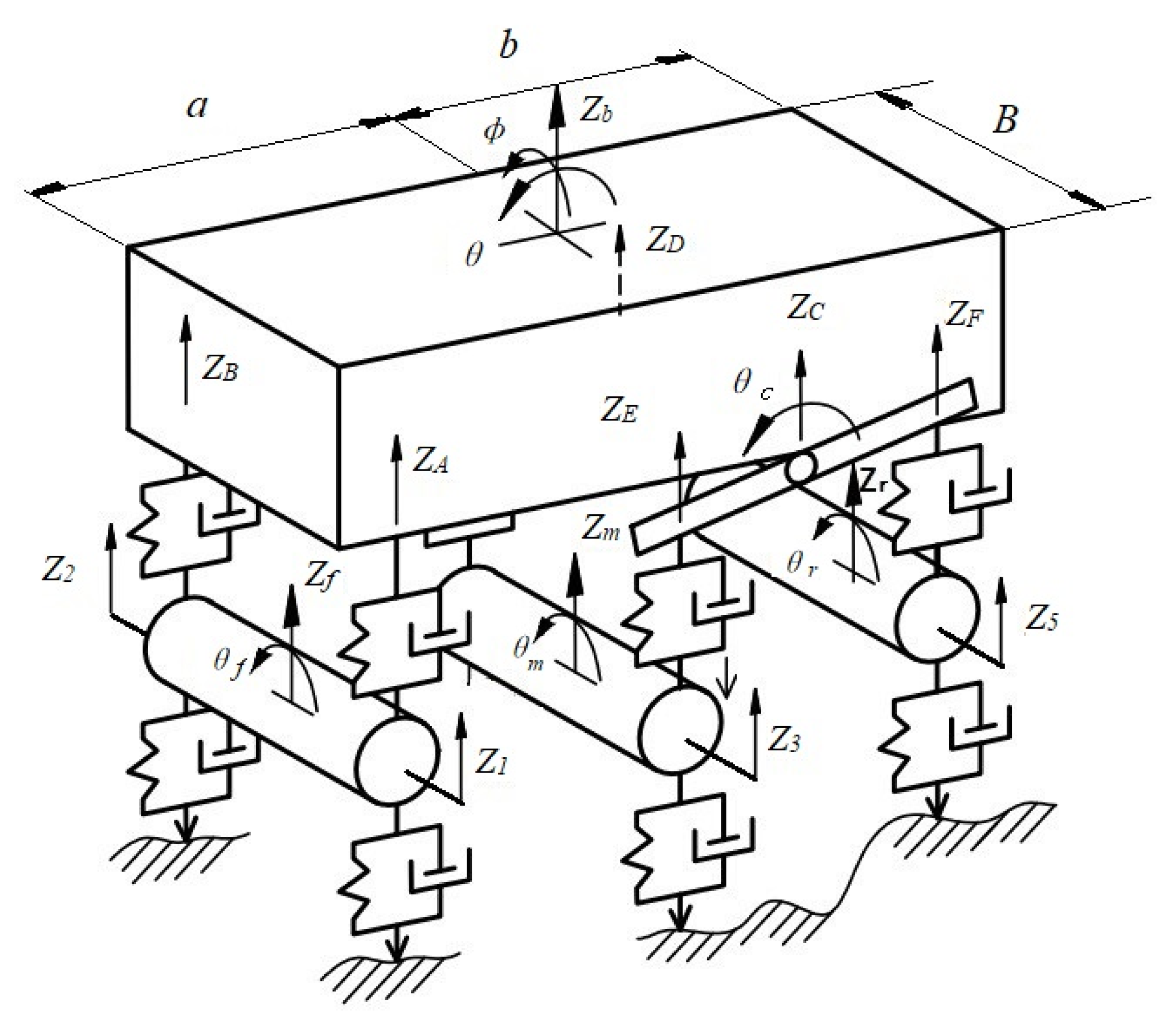
3.1. Eleven-DOFs Dump Truck Model

The dump truck is simplified to an 11-DOFs model comprising three DOFs associated with the vehicle body (Z_b, θ, Φ), six DOFs associated with the bounce and rolling motions of three integral axles (Z_A, Z_B, Z_C, Z_D, Z_E, Z_F), and two DOFs describe the pitch motions of the balanced suspension (θ_C, θ_D), as seen in Figure 6.

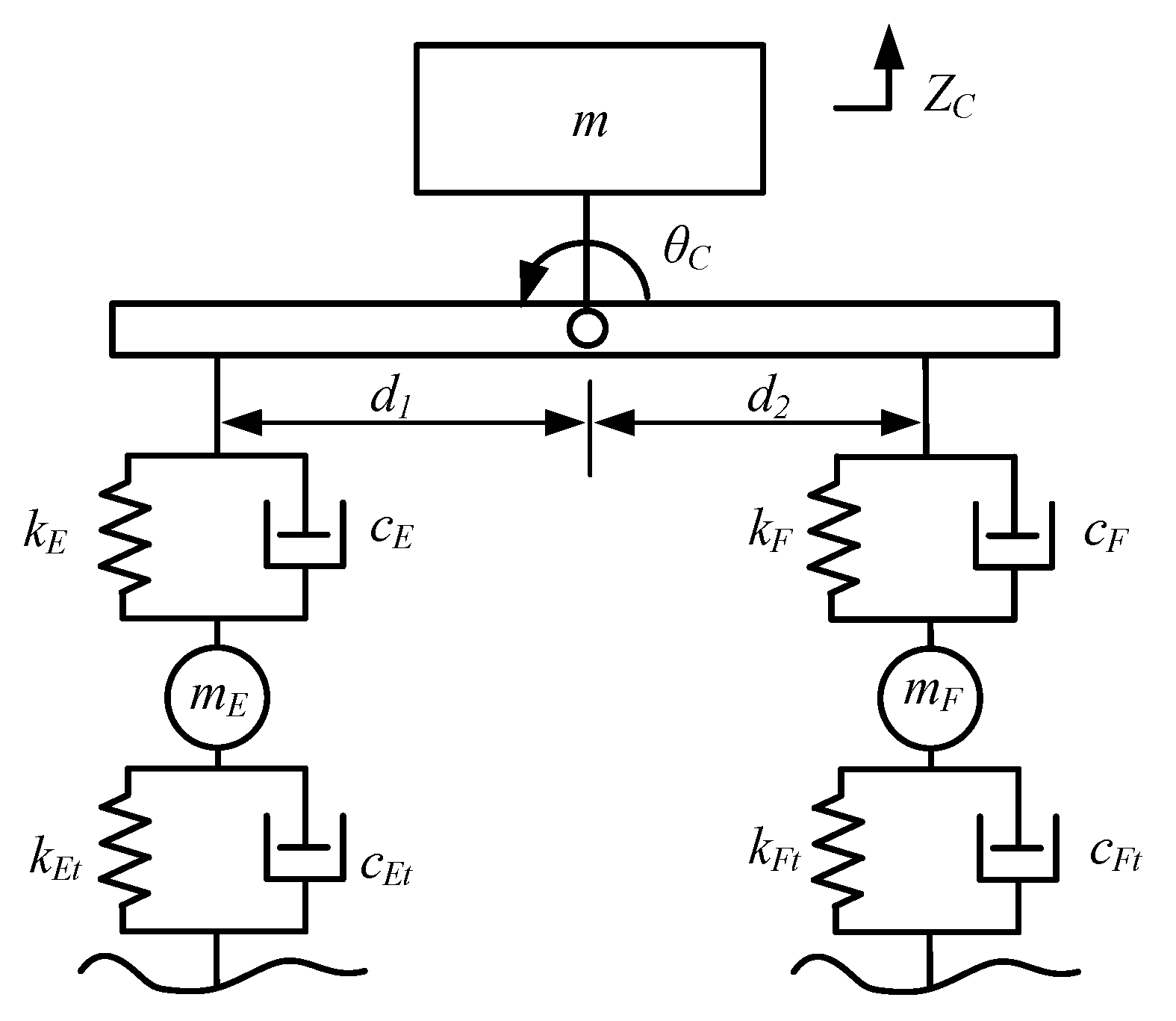
To simplify the modeling of the balanced suspension, the leaf spring is divided into two separate stiffnesses (k_E and k_F) and damping (c_E and c_F). Both ends of the leaf springs are separately linked with the front and rear axle through the rigid stabilizer rod. The front and rear axle vibrations are coupled together with the stabilizer rod [33]. The equivalent balance suspension model is shown in Figure 7.

The dynamic model of the dump truck, considering the integral axle and the balanced suspension, can be written in matrix form as:

$$M\ddot{Z}+C\dot{Z}+KZ=K_t{Q}_g+C_t{\dot{Q}}_g,$$

(3)

where M is the matrix representing vehicle body mass, Z is the vector of vehicle dynamic responses, C is the matrix of vehicle damping, K is the stiffness matrix of the vehicle system, C_t is the matrix of tire damping, K_t is the stiffness matrix of the tire and Q_g is the vector of displacement inputs acting on the tires.

The differential equations of Equation (3) can be transformed into the state space equation (Equation (4)) to facilitate the simulation, reducing the need for solution time and computing resources under the premise of ensuring system integrity and accuracy.

$$\{\begin{array}{l}\dot{x}=Ax+Bu\\ Y=Cx+Du\end{array},$$

(4)

The conventional method for equation transformation is achieved by selecting an appropriate intermediate variables x, regardless of the derivative term in the input variable u. The road roughness input Q_g was directly converted into the force input acting on the vehicle $K_t{Q}_g+C_t{\dot{Q}}_g$ = f(t) through numerical differential operation. Then:

$$\dot{x}=\left[\begin{array}{cc}0& I\\ -M^{-1}K& -M^{-1}C\end{array}\right]x+\left\{\begin{array}{c}\stackrel{̯}{\mathbf{0}}\\ M^{-1}\end{array}\right\}f(t),$$

(5)

where I and 0 represent identity and null matrices with similar dimensions as the property matrices, respectively; $\stackrel{̯}{0}$ is a null column vector whose length is the same as that of forcing vector f, and x is a vector containing the states (displacement and velocity vectors). The state variables x were selected as Equation (6):

$$\begin{array}{ll}x& =[Z,\dot{Z}]\\ & =[Z_b,\theta ,\varphi ,Z_f,{\theta }_f,Z_m,{\theta }_m,Z_r,{\theta }_r,{\theta }_C,{\theta }_D,{\dot{Z}}_b,\dot{\theta },\dot{\varphi },{\dot{Z}}_f,{\dot{\theta }}_f,{\dot{Z}}_m,{\dot{\theta }}_m,{\dot{Z}}_r,{\dot{\theta }}_r,{\dot{\theta }}_C,{\dot{\theta }}_D]\end{array},$$

(6)

Although input order reduction has been realized in Equation (5) via the conversion from $K_t{Q}_g+C_t{\dot{Q}}_g$ to f(t), the essence of this order reduction is an approximate computational process of a numerical differentiation algorithm based on the Runge-Kutta method. Order reduction itself could cause truncation error input and reduce the reliability and accuracy of the system output. Therefore, to oversimplify the input vector, it is essential to keep the input derivative for obtaining reliability and accuracy.

At present, the transformation from a single-input single-output (SISO) differential equation containing an input derivative to state space representation is achieved mainly by selecting an appropriate intermediate variable. Based on the SISO transformation method, the input, output variable, and the status variable are expanded to the vector; the variable of each system is expanded to the coefficient matrix, and matrix operations are introduced into the conversion process. Then, it became possible to eliminate the input derivatives of multivariable equations, ${\dot{Q}}_g$, and the state-space equation was achieved, as shown in Equation (7):

$${\dot{x}}_2=\left[\begin{array}{cc}0& I\\ -M^{-1}K& -M^{-1}C\end{array}\right]x_2+\left\{\begin{array}{c}{M}^{-1}Ct\\ M^{-1}Kt-M^{-1}C\times M^{-1}Ct\end{array}\right\}{Q}_g,$$

(7)

where the state variable x₂ was selected as Equation (8):

$$x_2=[Z,\dot{Z}-b_{1}Q],$$

(8)

After obtaining the state coefficient matrix $A=\left[\begin{array}{cc}0& I\\ -M^{-1}K& -M^{-1}C\end{array}\right]$ and the input matrix, $B=\left\{\begin{array}{c}{M}^{-1}Ct\\ M^{-1}Kt-M^{-1}C\times M^{-1}Ct\end{array}\right\}$, the appropriate output state matrix C and the output control matrix D (general definition D = 0) were specified via the state space ss.m function in MATLAB, and an 11-DOFs state-space model of a dump truck was built on the basis of Equation (7).

The state matrix A contains all the characteristic information of the model. Therefore, by decomposing A, the modal natural frequency fn, damping ratio ξ, and the modal vector v can be obtained.

3.2. Influence of Suspension Faults on Modal Parameters

During the long-term operation of the vehicle, load conditions and environmental factors can cause fault phenomena such as cracks and breaks in leaf springs, resulting in changes in the performance parameters of the suspension springs and a decrease in spring stiffness. To realize the suspension fault identification based on modal parameter analysis, it is essential to first understand the specific influence of the fault on the modal parameters. Therefore, it is necessary to calculate the modal parameters of the suspension system, i.e., natural frequency, damping ratio and mode shape, under different spring stiffnesses through simulation in MATLAB (R2017a, MathWorks, Natick, MA, USA).

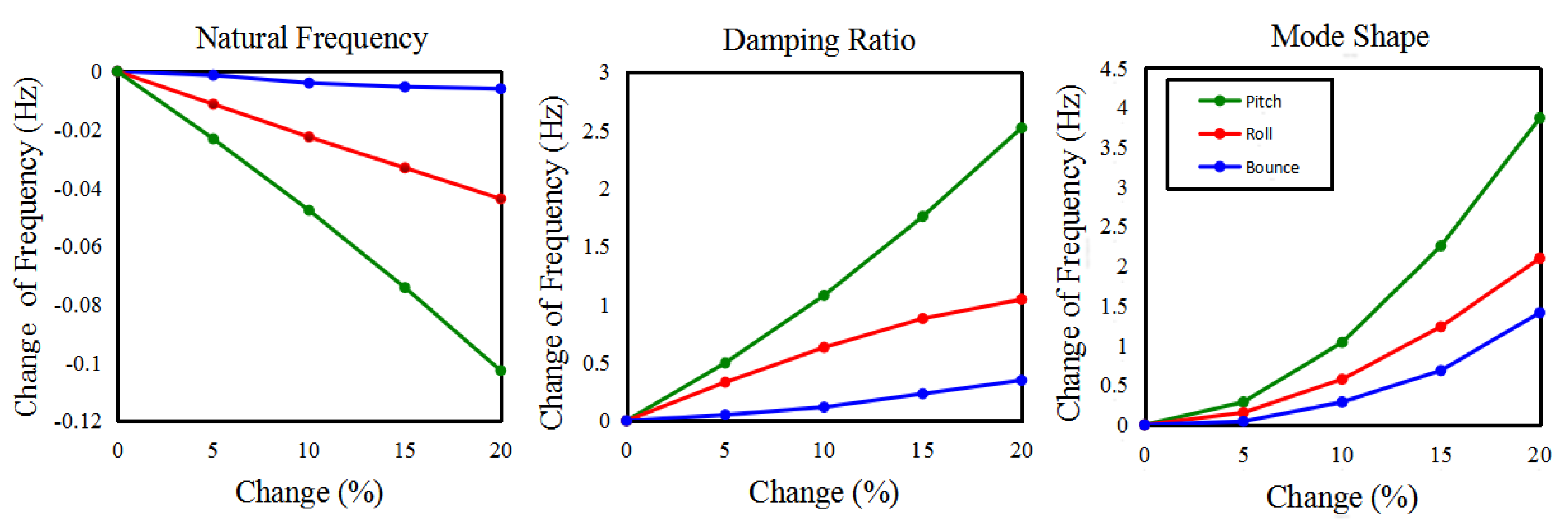
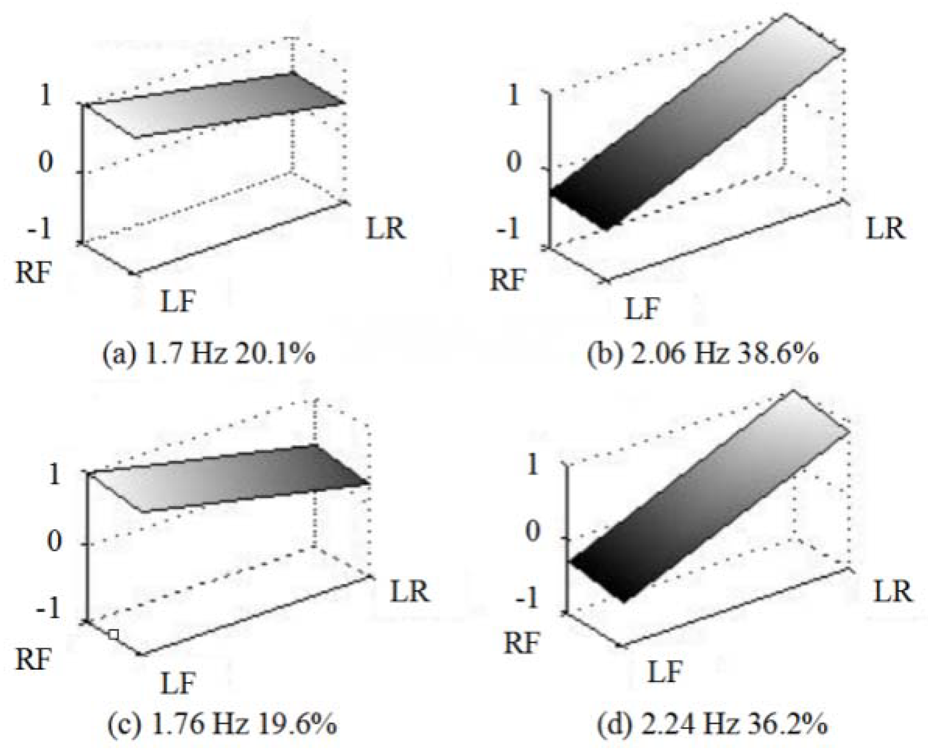
Firstly, the stiffness of the left rear spring is changed from 0% to 20% in the model to simulate spring failure and to study its effect on modal parameters. Figure 8 shows the changes in natural frequency, damping ratio and mode shapes caused by the drop in spring stiffness when the left rear leaf spring fails; the blue line represents the bounce mode, the green line represents the pitch mode and the red line represents the roll mode.

It can be seen from the first three modes that when the stiffness of the left rear spring is weakened, the natural frequencies of all three decreases to varying degrees, among which the pitch mode changes the most. Because of the small amplitude of the natural frequency variation, it is difficult to obtain accurate measurements in practical applications. The damping ratios of all three modes increased significantly, but the above suggested that the identification error of the damping ratio is larger than that of the other two. That is, the identified result can hardly reflect the actual change in damping ratio, so it is not suitable as an indicator of fault diagnosis. From the change of the vibration mode shapes in the three orders of modes in Figure 8, due to the mode shapes being considered as eigenvectors, the values are dimensionless, and the changes are obvious. This obvious feature can be used to judge the fault, and from the previous analysis in Section 2.2, the identification error of the modal mode is relatively small and thus suitable as a monitoring indicator.

It can be seen from the changes in the mode shape in Figure 8 that as a feature vector, the value of the mode shape is dimensionless and its variation is more obvious. This distinctive feature can be used to diagnose the fault and is suitable as a monitoring indicator.

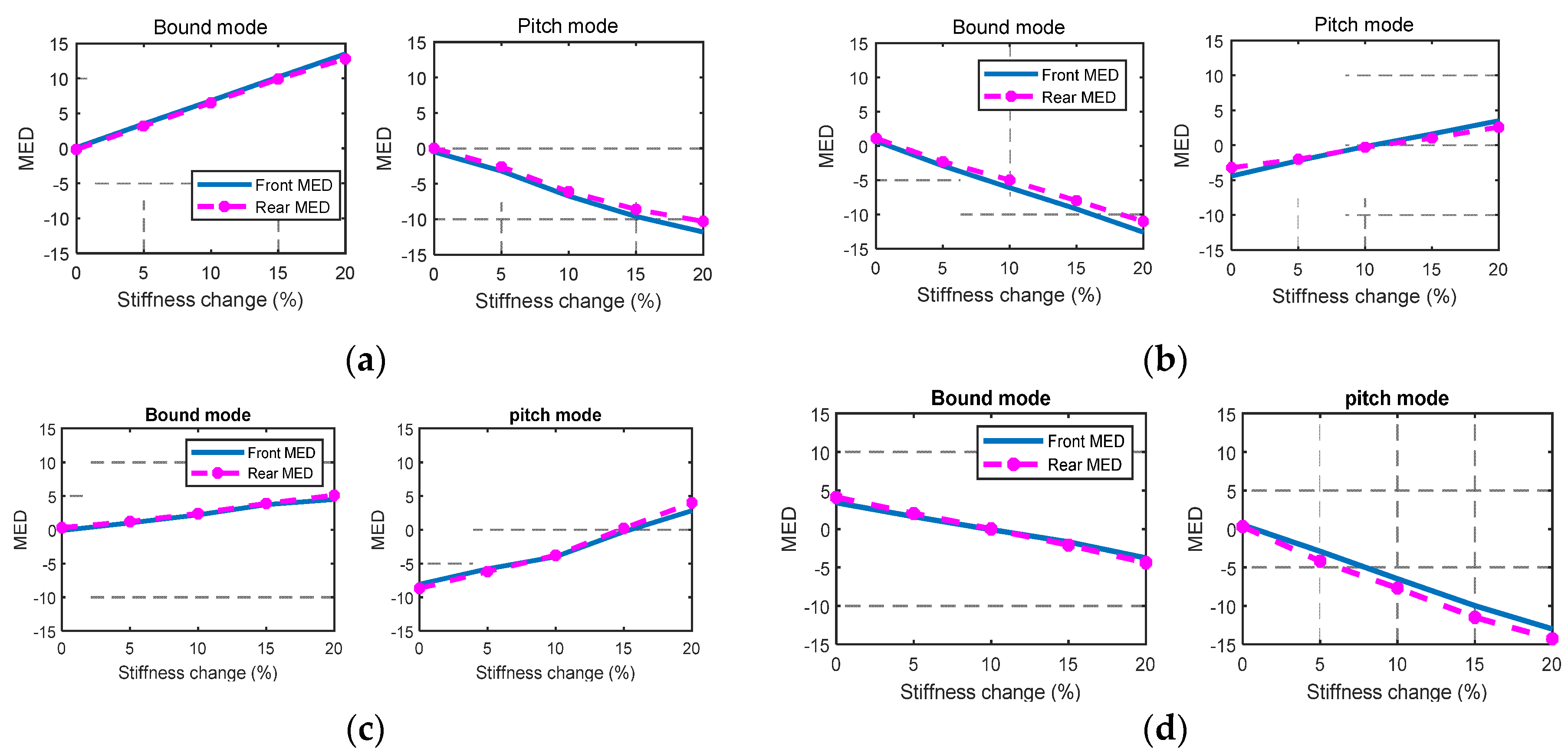
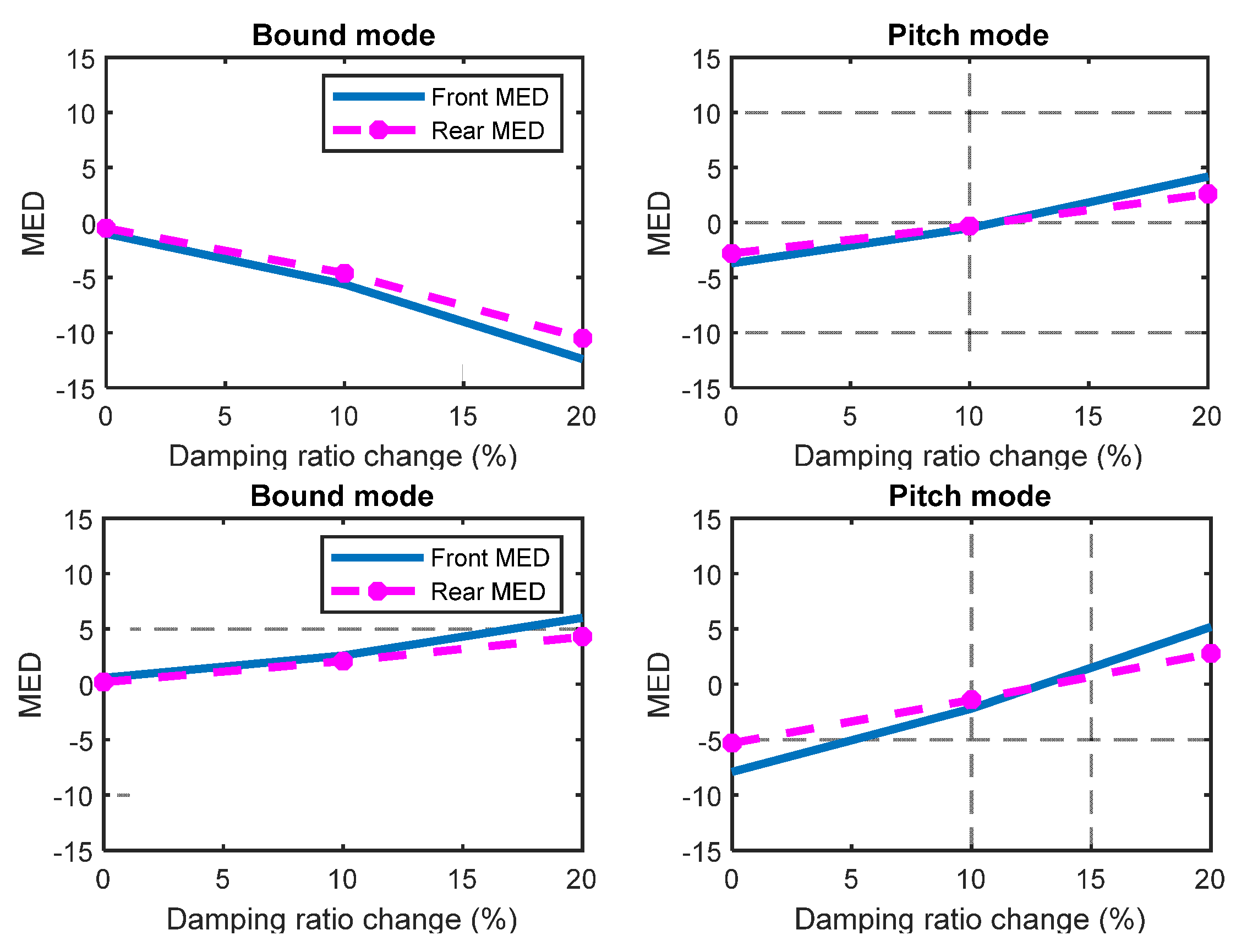
Then, the variation called modal energy difference (MED) is proposed to reveal the faults of suspension system more straightforwardly. In order to convey the imbalance of the mode shapes between the left and right sides, the rolling trends of mode shape are denoted as the differential of square of two mode shape, which is called modal energy difference (MED) in the following section. The MED between the left and right suspensions in bounce mode can be defined as Equation (9).

$$\begin{array}{l}d{E}_{bf}=2[(v_a^2-v_b^2)/(v_a^2+v_b^2)]\\ d{E}_{br}=2[(v_c^2-v_d^2)/(v_c^2+v_d^2)]\end{array},$$

(9)

where in, $d{E}_{bf}$ represents the difference between the vibration modes of left and right suspensions in front of the vehicle in the bounce mode, and $d{E}_{br}$ represents the MED in rear suspensions.

In Figure 9, the solid line is the MED between the two front suspensions and the dashed line represents the corresponding MED at the rear of the vehicle. The left and right sides of each figure respectively represent the modal energy changes in the first-order mode (bounce mode) and the third-order mode (pitch mode).

As shown in Figure 9a, when the left front wheel leaf spring fails, the difference in modal energy in the bounce mode increases by about 15%, and the difference in modal energy in the pitch mode drops by about 10%. When the right front wheel leaf spring fails (Figure 9b), the modal energy of the bounce mode decreases by about 10%, while the modal energy of the pitch mode increases from −5% to 3%, which is opposite to the trend presented in the two-order mode of the left front leaf spring. When the left rear leaf spring fails (Figure 9c), the modal energy of bounce mode increases by 3%, and the pitch mode increases from −7% to 3%. As shown in Figure 9d, the decrease in the stiffness of the right rear leaf spring causes a decrease in the modal energy of two modes, wherein the pitch mode decreases by 15%.

It can be seen that the weakening of the leaf springs at different positions of the vehicle can cause different changes in modal energy, because the change of spring stiffness at different positions will cause the vehicle to roll in different directions. It can be concluded that the modal energy difference is sensitive to leaf spring failure in both the bounce and pitch modes. Moreover, the position of the fault and the magnitude of the change in stiffness can be determined by the change in the modal energy difference.

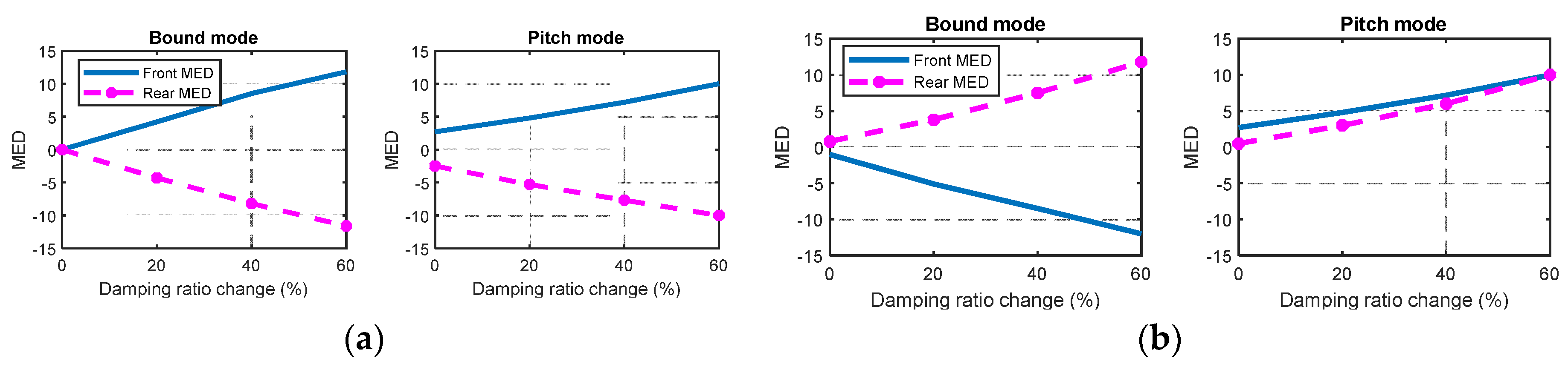
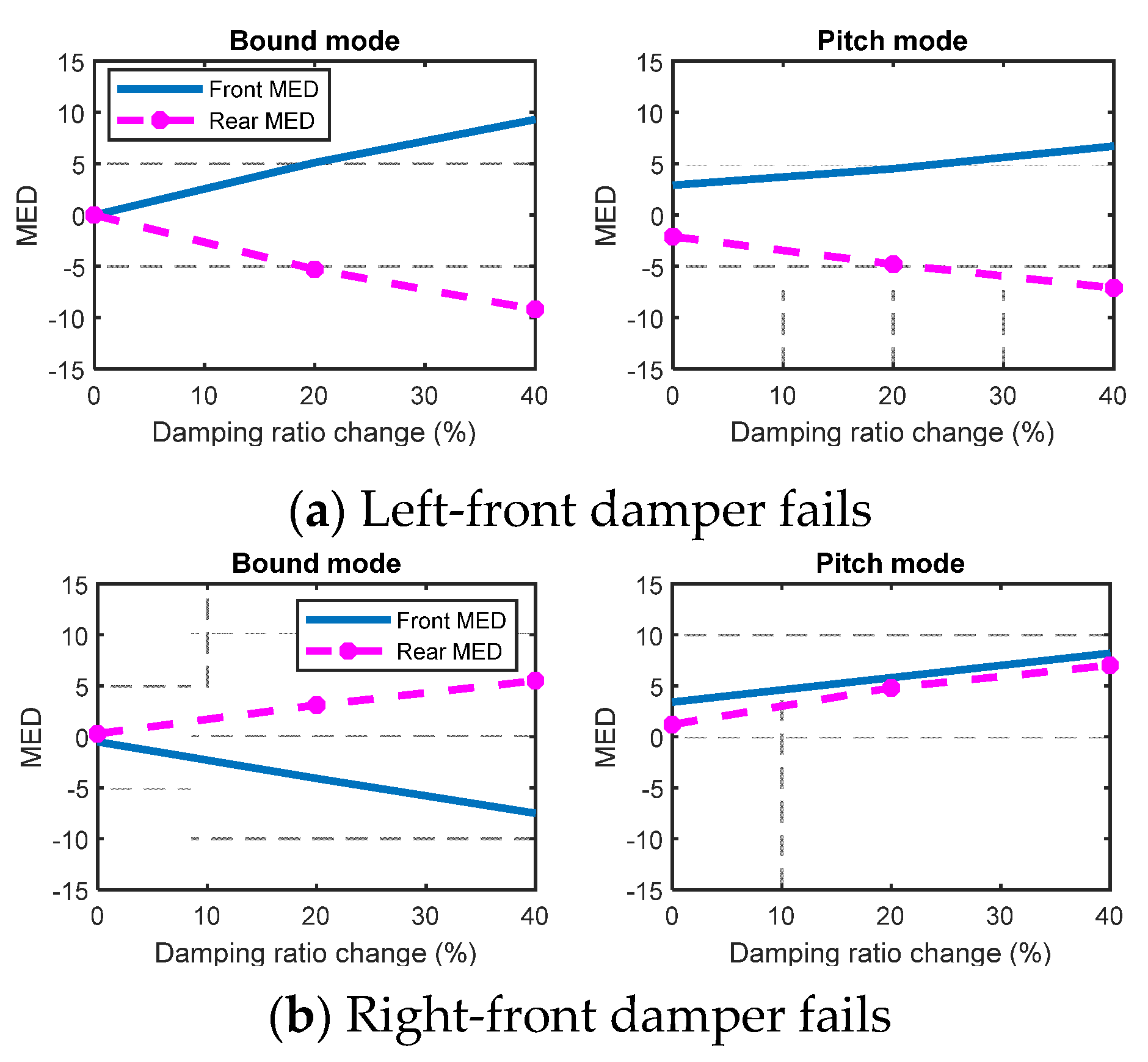
In order to simulate the influence of the damper fault on the modal parameters, the damping value of the shock absorber is gradually reduced from the original 100% to 30%.

As the damping of the left-front damper decreases, as seen in Figure 10a, the MED of the front and rear in the bounce mode presents a diametrically opposite trend. In the pitch mode, the MED of the front side gradually increases with the decrease of the damping value, and that of the rear side gradually decreases. If the right-front damper fails (Figure 10b), the MED in the bounce mode exhibits a tendency opposite to that of left-front side. In the pitch mode, unlike the left-front damper failure, the MED of the front and rear side increases slightly with the decrease of the damping.

It can be seen that the modal energy difference can clearly indicate the damping changes in a shock absorber and reveal the fault behind it. Therefore, the damper failure can be effectively monitored and diagnosed by the method proposed in this paper.

To summarize the tendencies of stiffness and damping ratio in the

Table 3. Tendencies of stiffness and damping ratio.

	Left				Right
	Bounce Mode		Pitch Mode		Bounce Mode		Pitch Mode
	Front MED	Rear MED	Front MED	Rear MED	Front MED	Rear MED	Front MED	Rear MED
Front spring	+	+	-	-	-	-	+	+
Rear spring	+	+	+	+	-	-	-	-
Damper	+	-	+	-	-	+	+	+

, we can see the positive and negative direction is distinctive in every situation. This shows the proof that MED can indicate the faults.

It strongly suggests that the modal energy differences are susceptible to stiffness changes and damping changes. Furthermore, the diverse trends of modal energy correspond to the occurrence of different faults, which help to achieve the purpose of fault diagnosis positioning and condition monitoring.

3.3. Verification of ACS-SSI Applied on MED

To further verify the correctness and accuracy of the proposed ACS-SSI algorithm, the failures of the leaf spring and the damper were simulated for error analysis. A noise signal with signal-to-noise ratio (SNR) equaling two is added to a select normal vibration response to simulate the fault vibration signal. The sampling frequency of the simulation system is 200 Hz, the sampling time is 20 s, and the average correlation calculation is carried out 50 times. Then, the proposed ACS-SSI algorithm was used to perform modal identification. The input data is set for a period of 100 s and averaged 50 times. Monte Carlo tests were performed 10 times for each simulation, and its corresponding identification error is shown in

Table 4. Identification error of simulated suspension spring faults.

Stiffness Changes	0%	5%	10%	15%	20%
Natural Frequency Error	3.16%	2.28%	2.14%	2.07%	3.25%
Modal Shape Error	4.78%	3.67%	3.16%	2.96%	4.69%

and

Table 5. Identification error of simulated absorber faults.

Damping Changes	0%	20%	40%	60%
Natural Frequency Error	4.32%	3.34%	5.53%	3.45%
Modal Shape Error	3.46%	2.64%	4.28%	2.86%

.

It can be seen from Table 4 and Table 5 that the identification error is always within a reasonable range, and the recognition error does not increase due to the change of the suspension parameters.

In order to investigate whether the different fault states can be clearly distinguished according to the modal energy difference in the presence of noise interference, the Monte Carlo test was repeated 50 times for three different spring stiffness conditions. The modal energy difference corresponding to the three spring stiffness states is shown in Figure 11.

4. Real-Scale Vehicle Tests and Result Analysis

The feasibility of the application of the ACS-SSI algorithm in fault identification and diagnosis of the dump truck suspension systems has been proven by a series of dynamic simulations. However, in the actual operation of the dump truck, there are many non-stationary, nonlinear dynamic characteristics and other mechanical vibration events aliased in the vibration response, which will affect the effectiveness of the diagnostic algorithm. To this end, it is necessary to further study the feasibility of the application of the ACS-SSI algorithm in the fault diagnosis of dump truck suspension systems through real-scale vehicle tests.

4.1. Sensor Arrangement

In order to accurately obtain the dynamic response of the suspension system, multiple acceleration sensors (Model No. X901, Sinocera Piezotronics, Inc., Yangzhou, China) needed to be placed at the axle, at the junction of the suspension and frame, and at the frame, as seen in Figure 12. During the operation of the dump truck, the suspension dynamic response is mainly caused by the vertical excitation of the road surface irregularity. Therefore, only unidirectional acceleration sensors were vertically arranged in all mounting points. Considering the structural characteristics of the dump truck with more degrees of freedom, 12 measuring points were symmetrically selected on both sides of the vehicle, including: the front and rear lifting lugs of front suspension, front axle (unsprung), the fourth beam of frame and the intermediate and rear axles (unsprung). The specific mounting position of the acceleration sensors on the left side of the suspension is shown in Figure 12. All of the vibration signals were recorded simultaneously by a multiple channel acquisition system (Model No. YMC9232, YMC Piezotronics, Inc., Yangzhou, China), and thereafter processed offline for making corresponding comparisons against 11-DOFs dynamic model predictions. In keeping with the sampling rate of the simulation system, the frequency of data acquisition is set to 200 Hz.

4.2. Testing Program

In order to verify the identification accuracy and robustness of the ACS-SSI algorithm under complex operating conditions and a strong noise background, tests under various suspension faults were carried out. Suspension faults were identified by analyzing the vibration response caused by random excitation of the road surface roughness. The real-scale vehicle testing programs under the condition of leaf spring failure (stiffness weakening) and shock absorber failure (damping reduction) are designed respectively. The two sets of testing cases are as follows:

In the first case, named Case 1, the left rear suspension spring was replaced by two springs with 80% and 90% stiffness of the original spring to simulate a suspension failure. It should be noted that, corresponding to the simulation results, the sampling length of the test data for each case is 200 s/times × 100 times = 20,000 s.

In the second case (Case 2), the left and right dampers of the front suspension were replaced by adjustable dampers. The sampling length of each test is the same 20,000 s.

Table 6. Changes of damping in the test.

State	Change of Left Front Damping	Change of Right Front Damping	Vehicle Speed
1	0%	0%	30 km/h
2	20%	0%	30 km/h
3	40%	0%	30 km/h

summarizes the changes of damping in the experiments. The damping of the adjustable damper can be set to three states, and State 1 is the baseline state. The damping value of State 1 to State 3 decreases from 100% to 60%.

4.3. Test and Result Analysis

4.3.1. Leaf Spring Failure (Case 1)

Firstly, the mode shapes and modal energy differences of the leaf spring with and without failure were analyzed. The modal frequencies and mode shapes of the baseline suspension and Case 1 were compared, and the results are shown in Figure 13.

Figure 13a,b shows the bounce and pitch mode vibration shapes at baseline; Figure 13c,d show the bounce and pitch mode shapes of the spring with 80% stiffness. It is apparent that the amplitudes of pitch and roll motions in Figure 13c,d are greater than that in Figure 13a,b, which verifies the results obtained by the simulation.

Then, the modal energy difference in bounce and pitch mode was obtained to highlight the change of stiffness. It can be seen from Figure 14 that the MED differences change with the stiffness of the faulty suspension spring. It can be concluded that based on the ACS-SSI modal identification method, the spring stiffness fault can be diagnosed by the change of the modal energy difference. In practical applications, appropriate test calibration for different vehicle types and fault forms can make the algorithm more widely used and more suitable for online monitoring.

4.3.2. Damper Failure (Case 2)

According to the testing program, the damping of the left front suspension damper was adjusted to three different states. It can be seen from the comparison of the modal energy differences in Figure 15a that the MED of the front bounce mode exhibits a significant rise, while the MED of the rear side shows the opposite downward trend. In the pitch mode, the MED of front pitch mode gradually increases as the damping decreases, while the MED of rear pitch mode is slightly reduced.

Consistent with the simulation predictions in Section 3.3, the MED of rear suspension failure in the bounce mode exhibits a tendency opposite to that of front suspension failure. In the pitch mode, the MED of both the front and rear side increases slightly with the decrease of the damping, which is also consistent with the simulation prediction. This shows that when the rear side damper fails, the reduction of damping will exacerbate the rolling motion of the front suspension. The results identified from the test data are basically consistent with the simulation, indicating that the MED-based monitoring technology is effective for monitoring and diagnosis of the damper faults.

5. Conclusions

This paper proposes a fault identification method based on an average correlation signal based stochastic subspace identification (ACS-SSI) algorithm and verifies its application feasibility in fault diagnosis of dump truck suspension through a series of simulations and an experiment. The main conclusions can be made as follows:

• It can be concluded that the modal energy difference (MED) is sensitive to the leaf spring failure in both the bounce and pitch modes. Moreover, the position of the fault and the variation amplitude of stiffness can be determined by the combination of MED in bounce and pitch modes. The plus or minus sign of the MEDs can indicate the specific location of faults, and the magnitude of change in MED can characterize the severity of the fault.
• The change in MED caused by damping failure is different from that caused by stiffness failure, but its location and fault degree can still be effectively identified by the combined analysis of MED.

In conclusion, the front and rear MEDs in bounce and pitch modes can serve as a vector to indicate the location and severity of the fault that occurred in the dump truck suspension. It shows that the proposed average correlation signal based stochastic subspace identification (ACS-SSI) method can identify the changes in suspension modal parameters effectively with respect to different spring stiffness and damping ratio conditions, which paves a promising way for the application of vibration-based online fault diagnosis to commercial vehicles operating in poor working environments and complex operating conditions.

References

1. Sandu, C. Vehicle dynamics: Theory and applications. J. Guid. Control Dyn. 2010, 33, 287–288. [Google Scholar] [CrossRef]
2. Woodrooffe, J. Heavy Truck Suspension Dynamics: Methods for Evaluating Suspension Road Friendliness and Ride Quality. J. Commer. Veh. 1996, 105, 337–343. [Google Scholar]
3. Sun, W.; Li, J.; Zhao, Y.; Gao, H. Vibration control for active seat suspension systems via dynamic output feedback with limited frequency characteristic. Mechatronics 2011, 21, 250–260. [Google Scholar] [CrossRef]
4. Li, H.; Liu, H.; Gao, H.; Shi, P. Reliable Fuzzy Control for Active Suspension Systems with Actuator Delay and Fault. IEEE Trans. Fuzzy Syst. 2012, 20, 342–357. [Google Scholar] [CrossRef] [Green Version]
5. Lee, C.; Choi, S.W.; Lee, I.B. Variable reconstruction and sensor fault identification using canonical variate analysis. J. Process Control 2006, 16, 747–761. [Google Scholar] [CrossRef]
6. Bruni, S.; Goodall, R.; Mei, T.; Tsunashima, H. Control and monitoring for railway vehicle dynamics. Veh. Syst. Dyn. 2007, 45, 743–779. [Google Scholar] [CrossRef]
7. Yin, S.; Ding, S.; Haghani, A.; Hao, H.; Zhang, P. A comparison study of basic data-driven fault diagnosis and process monitoring methods on the benchmark tennessee eastman process. J. Process Control 2012, 22, 1567–1581. [Google Scholar] [CrossRef]
8. He, Q.P.; Qin, S.J.; Wang, J. A new fault diagnosis method using fault directions in fisher discriminant analysis. AIChE J. 2005, 51, 555–571. [Google Scholar] [CrossRef]
9. Wei, X.; Jia, L.; Liu, H. A comparative study on fault detection methods of rail vehicle suspension systems based on acceleration measurements. Veh. Syst. Dyn. 2013, 51, 700–720. [Google Scholar] [CrossRef]
10. Teppola, P.; Minkkinen, P. Possibilistic and fuzzy c-means clustering for process monitoring in an activated sludge waste-water treatment plant. J. Chemom. 1999, 13, 445–459. [Google Scholar] [CrossRef]
11. Detroja, K.; Gudi, R.; Patwardhan, S. A possibilistic clustering approach to novel fault detection and isolation. J. Process Control 2006, 16, 1055–1073. [Google Scholar] [CrossRef]
12. Orani, N.; Pisano, A.; Usai, E. Fault diagnosis for the vertical three-tank system via high-order sliding-mode observation. J. Frankl. Inst. 2010, 347, 923–939. [Google Scholar] [CrossRef]
13. Zhao, Y.; Lam, J.; Gao, H. Fault detection for fuzzy systems with intermittent measurements. IEEE Trans. Fuzzy Syst. 2009, 17, 398–410. [Google Scholar] [CrossRef] [Green Version]
14. Karimi, H.R.; Zapateiro, M.; Luo, N. A linear matrix inequality approach to robust fault detection filter design of linear systems with mixed time-varying delays and nonlinear perturbations. J. Frankl. Inst. 2010, 347, 957–973. [Google Scholar] [CrossRef] [Green Version]
15. Gao, C.; Zhao, Q.; Duan, G. Robust actuator fault diagnosis scheme for satellite attitude control systems. J. Frankl. Inst. 2013, 350, 2560–2580. [Google Scholar] [CrossRef]
16. Dong, H.; Wang, Z.; Lam, J.; Gao, H. Fuzzy-model-based robust fault detection with stochastic mixed time delays and successive packet dropouts. IEEE Trans. Syst. Man Cybern. Part B Cybern. 2012, 42, 365–376. [Google Scholar] [CrossRef] [PubMed] [Green Version]
17. Gao, H.; Chen, T.; Wang, L. Robust fault detection with missing measurements. Int. J. Control 2008, 81, 804–819. [Google Scholar] [CrossRef]
18. Li, P.; Goodall, R. Model-based condition monitoring for railway vehicle systems. In Proceedings of the UKACC International Conference on Control, Bath, UK, 6–9 September 2004. [Google Scholar]
19. Hayashi, Y.; Tsunashima, H.; Marumo, Y. Fault detection of railway vehicle suspension systems using multiplemodel approach. J. Mech. Syst. Transp. Logist. 2008, 1, 88–99. [Google Scholar] [CrossRef]
20. Wei, X.; Lin, S.; Liu, H. Distributed fault detection observer for rail vehicle suspension systems. In Proceedings of the 24th Chinese Control and Decision Conference (CCDC), Taiyuan, China, 23–25 May 2012; pp. 3396–3401. [Google Scholar]
21. Juang, J.N.; Phan, M.Q. Identification and Control of Mechanical Systems. Appl. Mech. Rev. 2001, 55, 47. [Google Scholar] [CrossRef]
22. Pappalardo, M.C.; Guida, D. A time-domain system identification numerical procedure for obtaining linear dynamical models of multibody mechanical systems. Arch. Appl. Mech. 2018, 88, 1325–1347. [Google Scholar] [CrossRef]
23. Moonen, M.; Ramos, J. A subspace algorithm for balanced state space system identification. IEEE Trans. Autom. Control 1993, 38, 1727–1729. [Google Scholar] [CrossRef]
24. Dos Santos, P.L.; Ramos, J.A.; de Carvalho, J.L.M. Identification of linear parameter varying systems using an iterative deterministic-stochastic subspace approach. In Proceedings of the 2007 European Control Conference (ECC), Kos, Greece, 2–5 July 2007; pp. 4867–4873. [Google Scholar]
25. Moaveni, B.; Asgarieh, E. Deterministic-stochastic subspace identification method for identification of nonlinear structures as time-varying linear systems. Mech. Syst. Signal Process. 2012, 31, 40–55. [Google Scholar] [CrossRef]
26. Overschee, P.V.; Moor, B.D. Subspace Identification of Linear Systems; Springer: Berlin, Germany, 1996. [Google Scholar]
27. Sarmadi, S.A.N.; Venkatasubramanian, V. Electromechanical Mode Estimation Using Recursive Adaptive Stochastic Subspace Identification. IEEE Trans. Power Syst. 2014, 29, 349–358. [Google Scholar] [CrossRef]
28. Chen, Z.; Wang, T.; Gu, F.; Zhang, R.; Shen, J. The average correlation signal based stochastic subspace identification for the online modal analysis of a dump truck frame. J. Vibroeng. 2015, 17, 1971–1988. [Google Scholar]
29. Chen, Z.; Wang, T.; Gu, F.; Zhang, R. Characterizing the Dynamic Response of a Suspension Frame in a Heavy-Duty Dump Vehicle Based on an Improved Stochastic System Identification. Shock Vib. 2015, 2015, 1–15. [Google Scholar]
30. Dong, G.; Chen, J.; Zhang, N. Investigation into on-road vehicle parameter identification based on subspace methods. J. Sound Vib. 2014, 333, 6760–6779. [Google Scholar] [CrossRef]
31. Li, G.; Wang, T. Influence of long-waved road roughness on fatigue life of dump truck frame. J. Vibroeng. 2014, 16, 3862–3878. [Google Scholar]
32. Ngwangwa, H.M.; Heyns, P.S.; Breytenbach, H.G.A.; Els, P.S. Reconstruction of road defects and road roughness classification using Artificial Neural Networks simulation and vehicle dynamic responses: Application to experimental data. J. Terramech. 2014, 53, 1–18. [Google Scholar] [CrossRef] [Green Version]
33. Liu, J. Modeling and Simulation of Non-independent Suspension Vehicle. In Proceedings of the 2010 Asia-Pacific Conference on Power Electronics and Design, Wuhan, China, 30–31 May 2010; pp. 93–96. [Google Scholar]
Figure 1. Model of the three degrees of freedom (DOFs) system.
Applsci 08 01795 g001
Figure 2. Input signal of stochastic subspace identification (SSI) and average correlation signal based stochastic subspace identification (ACS-SSI). m1–3 = mass blocks. Acc: Acceleration Correlation.
Applsci 08 01795 g002
Figure 3. Identification error varying the damping ratio.
Applsci 08 01795 g003
Figure 4. Identification stabilization diagrams of ACS-SSI and SSI. PSD: Power Spectral Density
Applsci 08 01795 g004
Figure 5. Schematic diagram of simulation analysis.
Applsci 08 01795 g005
Figure 6. Eleven-DOFs dynamic model of a dump truck.
Applsci 08 01795 g006
Figure 7. Dynamic model of balanced suspension.
Applsci 08 01795 g007
Figure 8. Changes in natural frequency, damping ratio and mode shape caused by a left front spring fault.
Applsci 08 01795 g008
Figure 9. Change of modal energy difference (MED) caused by spring faults at different positions. (a): MED changes caused by faults in left front wheel; (b): MED changes caused by faults in right front wheel; (c): MED changes caused by faults in left rear wheel; (d): MED changes caused by faults in right rear wheel.
Applsci 08 01795 g009
Figure 10. Changes of MED in different positions of damper faults. (a): MED changes caused by faults in left-front damper; (b): MED changes caused by faults in right-front damper.
Applsci 08 01795 g010
Figure 11. Identification of rear modal energy difference.
Applsci 08 01795 g011
Figure 12. Position of accelerometers.
Applsci 08 01795 g012
Figure 13. Differences of mode shape between baseline and spring fault. RF: Right-Front; LF: Left-Front; LR: Left-Rear.
Applsci 08 01795 g013
Figure 14. Difference of rear MED between baseline and spring fault.
Applsci 08 01795 g014
Figure 15. Changes of MED caused by different damper faults.
Applsci 08 01795 g015