Error Correction for FSI-Based System without Cooperative Target Using an Adaptive Filtering Method and a Phase-Matching Mosaic Algorithm


State Key Laboratory of Precision Measurement Technology and Instruments, Tianjin University, Tianjin 300072, China
*
Author to whom correspondence should be addressed.
Appl. Sci. 2018, 8(10), 1954; https://doi.org/10.3390/app8101954
Submission received: 1 September 2018
/
Revised: 11 October 2018
/
Accepted: 14 October 2018
/
Published: 17 October 2018
(This article belongs to the Special Issue Precision Dimensional Measurements)
Abstract
:Featured Application
Absolute distance measurement and surface profiling.
Abstract
In our frequency scanning interferometry-based (FSI-based) absolute distance measurement system, a frequency sampling method is used to eliminate the influence of laser tuning nonlinearity. However, because the external cavity laser (ECL) has been used for five years, factors such as the mode hopping of the ECL and the low signal-to-noise ratio (SNR) in a non-cooperative target measurement bring new problems, including erroneous sampling points, phase jumps, and interfering signals. This article analyzes the impacts of the erroneous sampling points and interfering signals on the accuracy of measurement, and then proposes an adaptive filtering method to eliminate the influence. In addition, a phase-matching mosaic algorithm is used to eliminate the phase jump, and a segmentation mosaic algorithm is used to improve the data processing speed. The result of the simulation proves the efficiency of our method. In experiments, the measured target was located at eight different positions on a precise guide rail, and the incident angle was 12 degrees. The maximum deviation of the measured results between the FSI-based system and the He-Ne interferometer was 9.6 μm, and the maximum mean square error of our method was 2.4 μm, which approached the Cramer-Rao lower bound (CRLB) of 0.8 μm.
1. Introduction
Absolute distance measurement systems, which measure several tens of meters with microns uncertainties, are of significant interest in the field of metrology [1,2,3,4]. With the improvement of the external cavity laser (ECL), systems using frequency scanning interferometry FSI and the ECL play an important role in these fields: absolute distance measurement [5,6,7,8], imperfection detection [9], optical coherence tomography (OCT) [10], and three-dimensional surface profiling [11]. In our paper, attention is focused on absolute distance measurement.
An FSI-based absolute distance measurement system sends out a frequency-modulated signal to an object and receives the backscattering signal. The output is a low-frequency cosine wave in time domain that is affected by the tuning nonlinearity of the ECL [12,13]. Hence, in order to obtain precision in the order of microns, it is important for the ECL to provide linear frequency scanning over a broad tuning bandwidth [14]. However, because of the hysteresis and creep of the piezoelectric actuator (PZT), the ECL often shows tuning nonlinearity in practical situations. To eliminate the influence of the nonlinear tuning, many methods had been proposed [15,16,17,18,19].
In our paper, we sample the measurement interference signal at equidistant optical frequency points (EIOFs, namely sampling points) of the auxiliary interferometer with a long single mode polarization-maintaining fiber to eliminate the influence of tuning nonlinearity. This method is a common and effective method, but it creates a dispersion mismatch problem that results in target peak broadening. Fortunately, many dispersion compensation methods had been proposed and proved efficiently [20,21,22]. In our experiments without cooperate targets, we use an ECL that has been used for five years, so the SNR is low, and mode-hoping signals often occur. These bring new problems: erroneous sampling points and interfering signals. Our paper analyzes the influences of erroneous sampling points and interfering signals, and then an adaptive filtering method is proposed to eliminate the influences completely. In addition, a phase-matching mosaic algorithm and a segmentation mosaic algorithm are adopted to eliminate the phase jump and improve the data processing speed, respectively.
The article is organized as follows: Section 2 reviews the principle of the FSI-based system and discusses the measurement errors caused by erroneous sampling points and interfering signals. Then, an adaptive filtering method, a phase-matching mosaic algorithm, and a segmentation mosaic algorithm are proposed to eliminate the erroneous sampling points and phase jump and reduce the data processing time. In Section 3 and Section 4, the results of the simulation and experiment prove the efficiency of the methods that were proposed in Section 2. Finally, a brief conclusion is given in Section 5.
2. Theory
2.1. The Principle of FSI Using Frequency Sampling Method
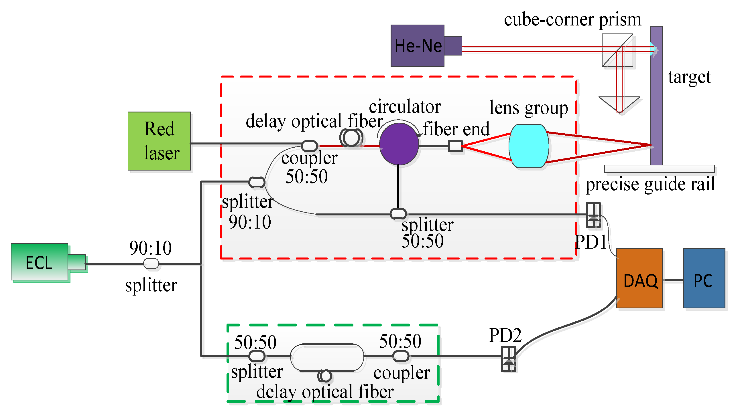
As is shown in Figure 1, the ECL has been used for five years and is connected with two interferometers. One is the auxiliary interferometer (as shown in the green box), whose output is used as the sampling signal to correct the tuning nonlinearity. The other is the measurement interferometer (as shown in the red box), whose output contains the information of measured distance. First, 10% power of the ECL goes into the auxiliary interferometer and the output is received by photo-detector 2 (PD2). Meanwhile, the remaining 90% of the power of the ECL goes into the measurement interferometer. Then, making use of a 90:10 optical splitter, 10% is used as the reference signal and 90% is used as the measurement light. Photo-detector 1 (PD1) obtains the output of the measurement interferometer. Finally, PD1 and PD2 convert the optical signals to the electric signals, and send the signals to the data acquisition card (DAQ). The He-Ne interferometer is used to verify the accuracy of our system.
The output of the measurement interferometer can be expressed as:
where is the amplitude of the measurement interference signal, is the initial frequency of the ECL, is the variation of the ECL instantaneous frequency, and is the time delay of the measurement interferometer.
Similarly, the ideal output of the auxiliary interferometer can be expressed as:
where is the amplitude of the auxiliary interference signal, and is the time delay of the auxiliary interferometer.
To eliminate the influence of the ECL tuning nonlinearity, taking the output of the auxiliary interferometer as the sampling signal yields:
where (k) is the variation of instantaneous frequency, k is the sampling point index, and N is the number of the ideal sampling point. So, the output of the measurement interferometer can be rewritten as:
Equation (4) by fast Fourier transform (FFT) yields:
where is the abscissa index of the peak point in the frequency spectrum of the measurement interferometer. When the dispersion is considered, according to John [23], it is easy to know:
where is the refractive index of air, is the measured distance, c is the speed of light in the vacuum, is the refractive index of the single mode fiber, is the length of the single mode fiber in the auxiliary interferometer, is the group velocity dispersion of the single-mode optical fiber, is the tuning rate of the ECL, is the group velocity, and t is the time.
So, the measured distance can be described as:
The second item in the right side of Equation (7) is caused by dispersion mismatch. Consequently, according to distance offsets, the absolute distance can be corrected by Equation (7).
2.2. The Influence of the Erroneous Sampling Points in the Auxiliary Interferometer
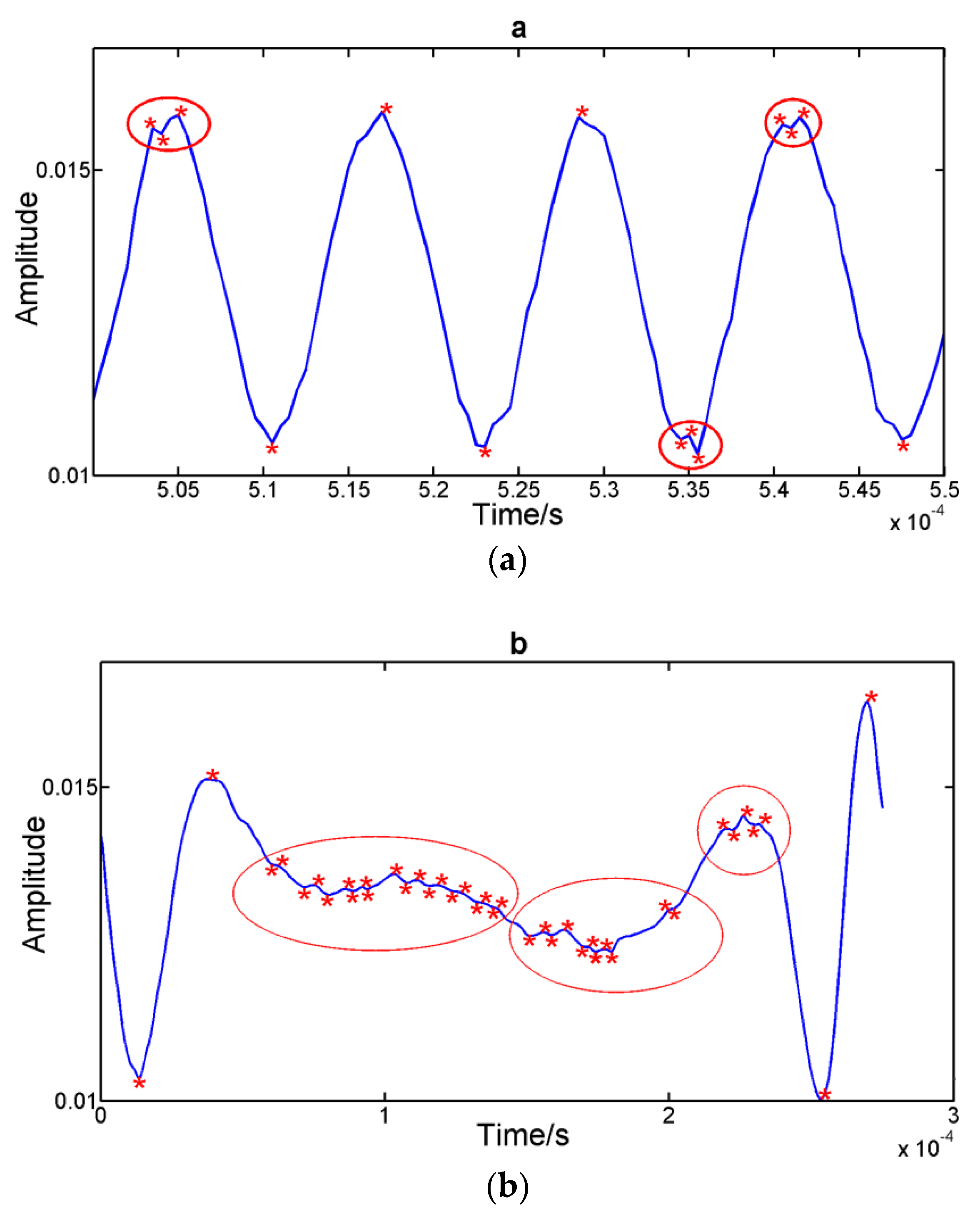
In the paper, we take the extreme points of the auxiliary interference signal as the sampling points. Figure 2 shows the extreme points of the auxiliary interferometer output in the experiments. Obviously, because of the influence of noises and mode-hopping signals, some of the extreme points are incorrect (as shown in the red circle section). Thus, the parameters N and in Equation (5) are different from their ideal values.
When there are noises and mode-hopping signals in the auxiliary interferometer, Equation (3) should be rewritten as:
where Ω is the phase deviation caused by all of the sampling points of the auxiliary interferometer output in the actual situation, and only part of the Ω is caused by the erroneous sampling points is not equal to zero, while is the number of the ideal sampling points, and is the total number of the sampling points in the actual situation. Thus, Equation (4) turns into:
Equation (9) by FFT yields:
where is the number of all of the erroneous sampling points in the auxiliary interferometer output, and is the abscissa value of the peak point in the frequency spectrum of the measurement signal in Equation (9).
If is much smaller than N, the second item on the left side of Equation (10) can be neglected. So, the measurement error caused by the erroneous sampling points of the auxiliary interferometer output can be shown as:
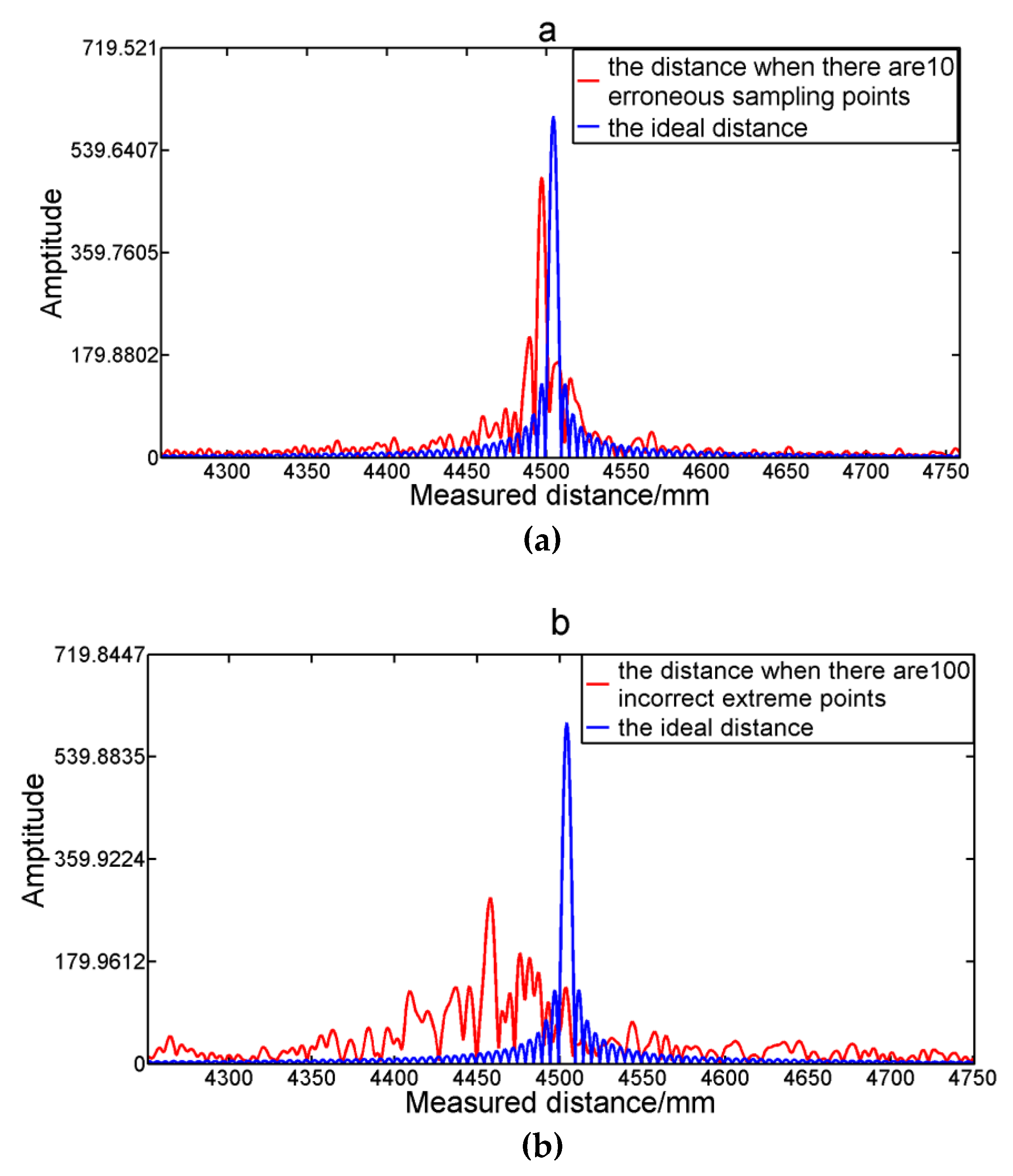
where is the measurement error caused by the erroneous sampling points of the auxiliary interferometer, is the measured distance when there are erroneous sampling points, and is the ideal measured distance when there are no erroneous sampling points. Figure 3a shows the comparison of the simulated result when there are 10 erroneous sampling points (the red line) and the ideal distance (the blue line). In our experiments, is 1.4682, is 1.0003, and is 20.05832 m. When the ideal value of P is 9000, N is 60,000, and is 10, the measured distance error is 758.9 μm, which is agreement with the theoretical measurement error of 760 μm, which is calculated by Equation (11). Obviously, the accuracy of the measurement distance is greatly affected. Besides, the main lobe energy of the spectrum decreases, and the side lobe’s energy increase. Hence, it is essential to eliminate the influence of the erroneous sampling points in order to ensure the accuracy.
As is shown in Figure 3b, if is 100, the second item on the left-hand side of Equation (11) can’t be neglected. In this situation, we cannot obtain the accurate measured distance.
2.3. The CRLB When There Are Interfering Signals and Noise in the Measurement Interferometer
Ignoring the influence of the erroneous sampling points in the auxiliary interferometer, when the system measures the non-cooperative target and there is noise in the measurement interferometer, Equation (4) turns into:
where denotes the Gaussian white noise (GWN) with an expectation of 0 and variance σ2 denotes the interfering signals, and is , is . The interfering signals are caused by the reflected lights from the circulator and the fiber end in Figure 1.
As shown in Figure 4, when our system measures a non-cooperative target, the measurement signal (the red line) becomes very weak, and the interfering signals (the blue line) are much stronger than the measurement signal. In addition, the frequencies of the interfering signals are not varying with the measured distances and are lower than the frequency of the measured signal, so we can use an appropriate low pass filter to delete them. Thus, the SNR of the measurement interferometer output can be shown as /σ2.
The Cramer–Rao lower bound (CRLB) is a method in the statistics and the variance of any unbiased estimator cannot be lower than the CRLB [23]. Therefore, we use the CRLB to evaluate our system. The likelihood function of can be expressed as:
The Fisher information is obtained as:
The CRLB on the variance of the measured distance is:
Accordingly, when there is GWN in the measurement interferometer, the CRLB on the standard deviation of measured distance can be shown as:
When the measured target is not a reflector or a corner prism and the incident angle is not zero, the SNR should be low, and the error caused by the GWN in the measurement interferometer can’t be ignored.
2.4. The Adaptive Filtering Method, the Phase-Matching Mosaic Algorithm, and the Segmentation Mosaic Algorithm
According to the analysis above, completely eliminating the erroneous sampling points of the auxiliary interferometer and the interfering signals in the measurement interferometer are essential in order to ensure the accuracy of our system. Thus, an adaptive filtering method and a phase-matching mosaic algorithm are proposed to ensure the accuracy, and a segmentation mosaic algorithm is used to improve the data-processing speed. The adaptive filtering method can be described as following.
- (1)
- Firstly, we make use of the Hanning window and the wavelet threshold filtering to depress the noises (such as the GWN) and the interfering signals in the auxiliary interferometer and measurement interferometer.
- (2)
- Then, we get the sampling points (all of the maximum and minimum extreme points of the auxiliary interference signal) and set appropriate thresholds to delete most of the erroneous sampling points caused by mode-hopping signals.
- (3)
- Lastly, according to the rule that the maximum and minimum values occur alternately, we remove the rest of the erroneous sampling points.
Step (1) is used to depress the noises and the interfering signals in the auxiliary interferometer and measurement interferometer. The Hanning window filtering method had been proved to be an effective method to depress the low and high frequency noise in an FSI-based system [10]. In our experiments, the measurement signal was very weak, and its frequency was varying with the measured distance, so we must use an adaptive filtering method to depress the GWN. The wavelet threshold filtering method is adopted in our paper. The mechanism of wavelet threshold filtering is based on the different properties of the wavelet coefficients of signals and noises on scales. To eliminate the noise, corresponding rules are adopted to deal with the nonlinear processing of the wavelet coefficients of the noise [24].
Step (2) and Step (3) are used to delete the erroneous sampling points caused by the mode-hopping of the ECL. Firstly, we get all of the sampling points in the auxiliary interferometer. The set of all of the sampling points can be described as:
where denotes a set of all of the sampling points, denotes a set of all of the maximum extreme points, and denotes a set of all of the minimum extreme points. Then, we find that the amplitude and the time interval of the erroneous sampling points is obviously smaller than the correct sampling points. Firstly, we set the amplitude thresholds to delete part of the erroneous sampling points, and the rest of the sampling points can be written as:
where denotes a set of the sampling points that contains part of the erroneous sampling points, A(xk) is the amplitude of the extreme point, is the maximum amplitude of the auxiliary interference signal, is the minimum amplitude of the auxiliary interference signal, k is the index of the extreme points, and S is the length of . Then, we set the time interval thresholds to delete part of the erroneous sampling points, and the rest of the sampling points can be written as:
where x denotes the sampling point in , T(xk) is the time interval of the extreme point, denotes the mean time interval of all of the points in , and K is the length of .
Lastly, we find that the rest of the erroneous sampling points do not follow the rule that the maximum and minimum values occur alternately. So, the set of the correct sampling points can be described as:
where denotes a set of the correct extreme points, k is the index of the correct extreme points, and M is the length of the . Thus, the measurement errors that are caused by the erroneous sampling points and the interfering signals are eliminated.
In addition, the phase-matching mosaic algorithm and the segmentation mosaic algorithm are used to eliminate the phase jump and improve the data-processing speed. After sampling the measurement signal with , phase jump occurs at the starting and ending point of each mode-hopping signal in the measurement interferometer [25]. To solve the problem, firstly we find the starting point and ending point of each mode-hopping signal by the time interval. Then, we use the Hilbert translation to exact the phase of the 10 points before the starting point and the 10 points after the ending point and compare their phases one by one. Lastly, we stitch the closest two points. When the tuning bandwidth, tuning speed, and sampling frequency of the data acquisition card are set, the required number of the sampling points is fixed. The first step of the segmentation mosaic algorithm is dividing the signal of the fixed length to 10 segment signals of the same length, namely:
Then, we use the adaptive filtering method and the phase-matching mosaic algorithm to progress them separately. Finally, the measured distance should be described as:
Each segment signal is one-tenth of the fixed length, so the time that FFT spent is greatly reduced.
3. Simulation
When there are noises and the mode-hopping signals in the auxiliary interferometer, the output of the auxiliary interferometer can be described as:
where simulates the actual output of the auxiliary interferometer, simulates the ideal output of the auxiliary interferometer, simulates the Gaussian white noise, awng is a function in Matlab that simulates the GWN, simulates the mode-hopping signals, Low(t) simulates the low-frequency noise, High(t) simulates the high-frequency noise, t is the sampling time, and simulates the variation caused by the tuning nonlinearity of the ECL. The sampling frequency of the simulation is 5 MHz, and the number of sampling points is 1 ×, which is the same with the experiments in Section 4.
When FSI-based system measures non-cooperative targets, the SNR of the measurement interferometer is low. We set the SNR of the measurement interferometer to 5 dB, which is the same with the SNR in the experiments, so the output of the measurement interferometer can be simulated as:
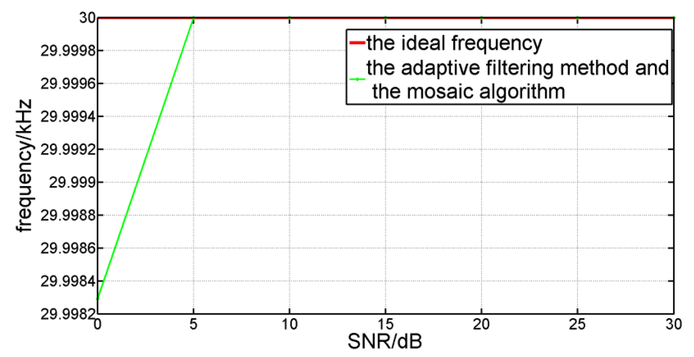
where simulates the actual output of the measurement interferometer, simulates the ideal output of the measurement interferometer, simulates the GWN, simulates the interfering signals, and is the variable caused by the ECL nonlinearity tuning. The ideal frequency is 30,000 Hz, and all of the signal processing was performed in MATLAB.
Figure 5 shows the comparison of the ideal frequency (the red line) with the simulated result of our method (the green line). When the SNR of the auxiliary interferometer ranges from 5 dB to 30 dB, the result of our method is the same with the ideal frequency. However, if the SNR is 0 dB, the result of our method is slightly smaller than the ideal frequency. In our experiments, the SNR of the auxiliary interferometer was about 25 dB, and our adaptive filtering method was effective in this situation.
4. Experiment and Analysis
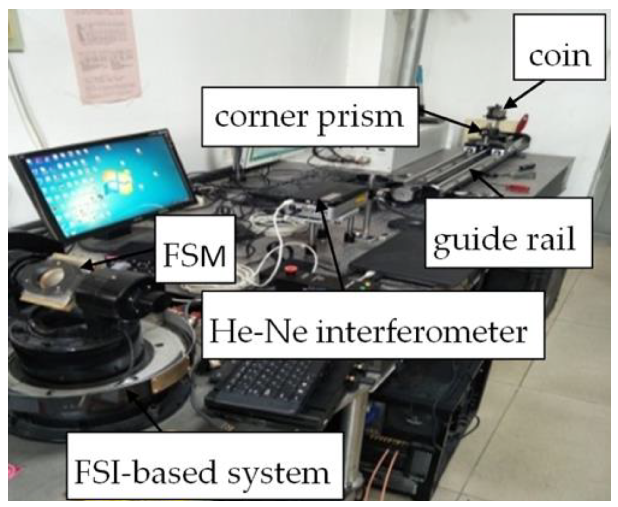
Figure 6 shows the setup of our experiments. It includes two parts: the FSI-based absolute distance measurement system, and the interferometer (Renishaw XL-80). The ECL has been used for five years, and mode-hopping of the ECL (NewfocusTLB-6728) always happens. In experiments, the power of the ECL was 8 mW, and the scanning range of the ECL was 1515–1535 nm. The optical frequency was set to sweep as a triangle at tuning rate of 100 nm/s. The sampling frequency of the DAQ (Gage CSE161G4) was 5 MHz, and the number of sampling points was 1 ×. The measured target was a 10-cent coin, and the incident angle of the measurement signal was 12 degrees, so the backward echo signal was very weak.
The He-Ne interferometer was used to verify the accuracy of our method. The cube-corner prism of the He-Ne interferometer and the target of the FSI system were both fixed on a slider. The slider moved along a precise guiderail, and the range of the guiderail was 1000 mm.
The measured result in Figure 4 consists of two parts. One was the distance from the ECL to the fast steering mirror (FSM) of our FSI-based system, and it can be obtained when the FSM was horizontal. Another was the measured distance from the FSM to the measured target, such as the results in Figure 7 and Figure 8. In our experiments, the former was 8385.432 mm. The measured distance in Figure 7 and Figure 8 was the measured result minus 8.385.432 mm.
Figure 7 shows the comparison of the experiment results between the method of Deng et al. [17] (part a) and the adaptive filtering method and the mosaic algorithm (part b) with the same experiment data. It proves the necessity and effectiveness of our method to deal with the noises and the mode-hopping signals.
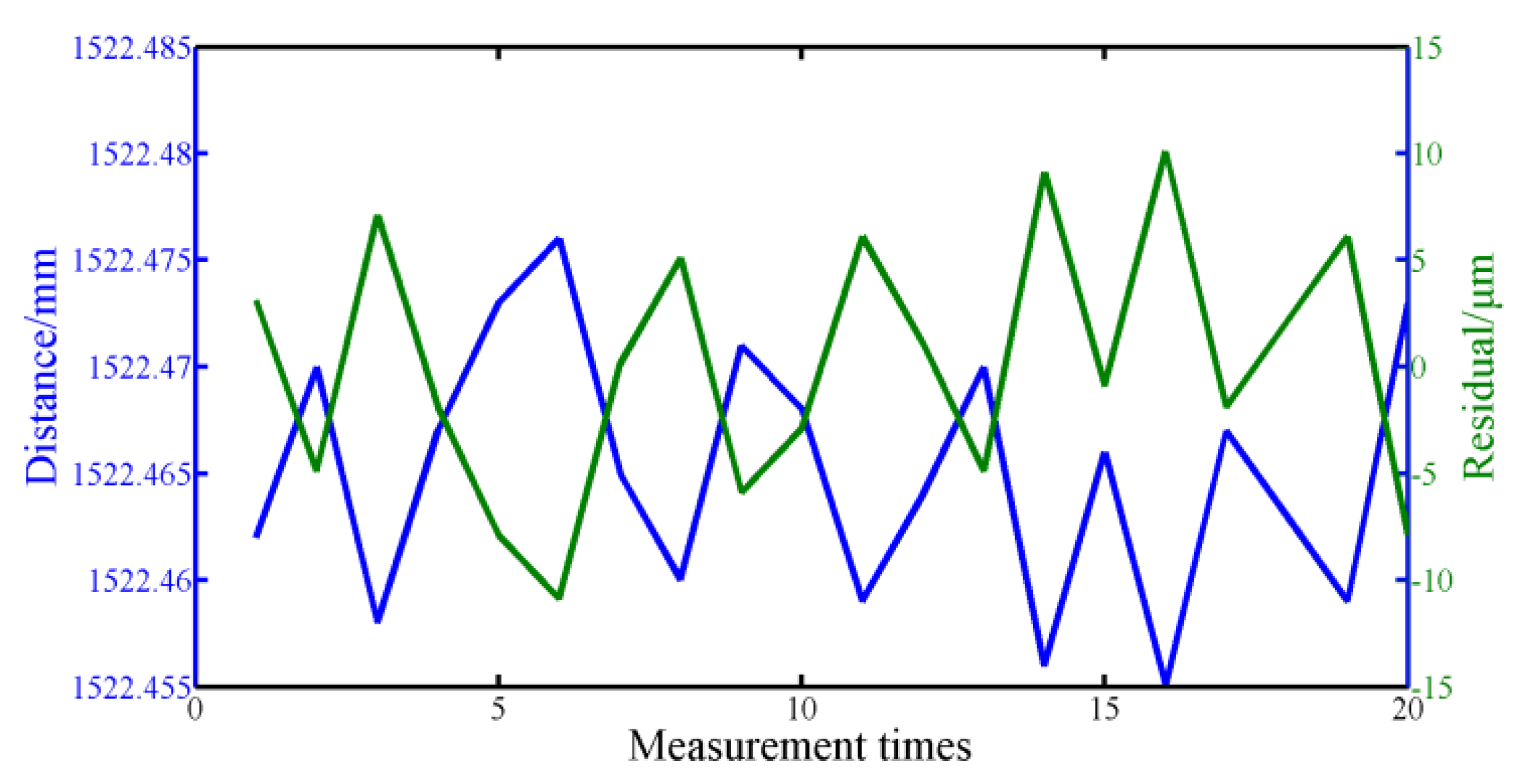
In order to analyze the stability of our method, we measured the coin 20 times at one position and used our adaptive filtering method and mosaic algorithm to progress the experiment data. As shown in Figure 8, the blue line denoted the results of 20 measurements, and the green line denoted the residuals. When there were noises, the mode-hopping signals and the interfering signals in our system, the statistical uncertainty of our method was 5.7 μm over 20 measurements, which was the same order as the result of Lu et al. [16].
To evaluate the accuracy of our method, the coin moved 62.45 mm every time, and totally moved seven times. The FSI-based system and the He-Ne interferometer simultaneously measured the displacement of the slider. So, our FSI-based system and the laser interferometer could use the same air refractive index. The measured results of the laser interferometer were used as the truth value of the moving distance. Figure 9 showed the difference between the measured results of our systemand the laser interferometer. The max relative error of our method was 9.6 μm. The relative error was attributed to the Abbe error, the air-path distance variation, and the optical dispersion error. In our experiment, the moving distance was less than 500 mm, so the Abbe error between the laser interferometer and our FSI-based systemwas less than 0.5 μm. The air-path distance variation was mainly caused by the variation of the air refractive index. The temperature, pressure and humidity in the experiments were basically stable, so the error caused by the air-path distance variation was within 1 μm. The optical dispersion error was originated from the optical frequency sweep of the ECL, and was compensated by Equation (7). According to Equation (7), the moving distance was 0.06245 m, was −23 ps2/km, and the tuning bandwidth was 10 nm, so the distance offset was 2.3 μm.
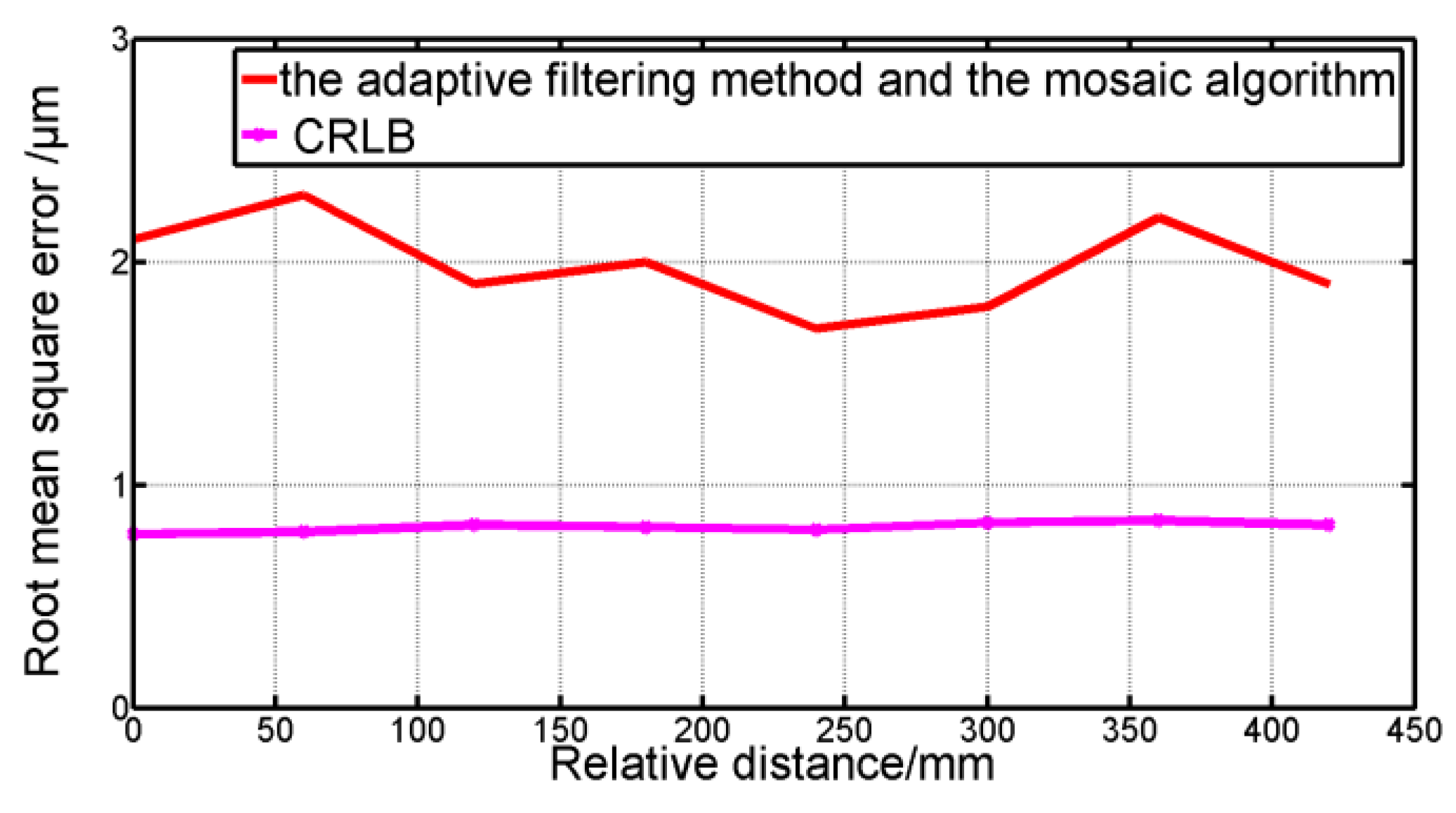
The CRLB was used to evaluate the performances of our system. In our experiments, was 1.4682, was 1.0003, was 20.05832 m, the SNR was 5 dB, and the ideal value of N was about 60,000. According to Equation (16), the CRLB was about 0.8 μm. Figure 10 showed the comparison of the measured root mean square error (MSEs) at eight positions with the CRLB. The red and pink data denoted the MSE obtained by the results of six independent measurements and the CRLB of ranging estimation, respectively. The max MSE based on our method at eight different placements was 2.4 μm, which approached the CRLB of 0.8 μm.
5. Conclusions
In our FSI-based system, the ECL has been used for five years. Thus, the SNR of the ECL is low, and the mode-hopping signals often occur. In addition, the influence of the interfering signals cannot be neglected when the system measures non-cooperative targets. To ensure the precision of our system, it is essential to delete the erroneous sampling points in the auxiliary interferometer and the interfering signals and phase jump in the measurement interferometer. So, the adaptive filtering method, the phase-matching mosaic algorithm, and the segmentation mosaic algorithm are proposed to solve the problems and improve the data processing speed. The results of our simulation prove the efficiency and applicability of our methods. In the experiments, the target was a coin and the laser interferometer (Renishaw XL80) was used to verify the efficiency of our method. The stability of our system was 5.7 μm over 20 measurements. The maximum deviation of the measured results between the FSI-based system and the He–Ne interferometer was 9.6 μm, and the maximum mean square error of our method was 2.4 μm, which approached the Cramer-Rao lower bound (CRLB) 0.8 μm.
Author Contributions
Conceived the Method and Wrote the Paper, X.-T.X.; Designed the Experiments, X.-H.Q.; Improved the Experimental Results, F.-M.Z.
Funding
Natural National Science Foundation of China (NSFC) (No. 51675380, No. 51775379), National Key Research and Development Plan(2018TFF0212702).
Conflicts of Interest
The authors declare no conflict of interest.
References
- Barwood, G.P.; Gill, P.; Rowley, W.R.C. High-accuracy length metrology using multiple-stage swept-frequency interferometry with laser diodes. Meas. Sci. Technol. 1999, 9, 1036–1041. [Google Scholar] [CrossRef]
- Stejskal, A.; Stone, J.A.; Howard, L. Absolute interferometry with a 670-nm external cavity diode laser. Appl. Opt. 1999, 38, 5981–5994. [Google Scholar]
- Le, F.S.; Salvadé, Y.; Mitouassiwou, R.; Favre, P. Radio frequency controlled synthetic wavelength sweep for absolute distance measurement by optical interferometry. Appl. Opt. 2008, 47, 3027–3031. [Google Scholar]
- Gao, R.; Wang, L.; Teti, R.; Dornfeld, D.; Kumara, S.; Mori, M.; Helu, M. Cloud-enabled prognosis for manufacturing. CIRP Ann. Manuf. Technol. 2015, 64, 749–772. [Google Scholar] [CrossRef] [Green Version]
- Abou-Zeid, A.; Pollinger, F.; Meiners-Hagen, K.; Wedde, M. Diode-laser-based high-precision absolute distance interferometer of 20 m range. Appl. Opt. 2009, 48, 6188–6194. [Google Scholar]
- Kinder, T.; Salewski, K.D. Absolute distance interferometer with grating-stabilized tunable diode laser at 633 nm. J. Opt. Apure Appl. Opt. 2002, 4, S364–S368. [Google Scholar] [CrossRef]
- Dale, J.; Hughes, B.; Lancaster, A.J.; Lewis, A.J.; Reichold, A.J.H.; Warden, M.S. Multi-channel absolute distancemeasurement system with sub ppm-accuracy and 20 m range using frequency scanning interferometry and gas absorptioncells. Opt. Express 2014, 22, 24869–24893. [Google Scholar] [CrossRef] [PubMed]
- Prellinger, G.; Meinershagen, K.; Pollinger, F. Spectroscopically in situ traceable heterodyne frequency-scanning interferometry for distances up to 50 m. Meas. Sci. Technol. 2015, 26, 084003. [Google Scholar] [CrossRef]
- Wang, L.T.; Iiyama, K.; Tsukada, F.; Yoshida, N.; Hayashi, K.I. Loss measurement in optical waveguide devices by coherentfrequency-modulated continuous-wave reflectometry. Opt. Lett. 1993, 18, 1095–1097. [Google Scholar] [CrossRef] [PubMed]
- Zheng, K.; Liu, B.; Huang, C.; Brezinski, M.E. Experimental confirmation of potential swept source optical coherence tomography performance limitations. Appl. Opt. 2008, 47, 6151–6158. [Google Scholar] [CrossRef] [PubMed] [Green Version]
- Baumann, E.; Giorgetta, F.R.; Deschênes, J.D.; Swann, W.C.; Coddington, I.; Newbury, N.R. Comb-calibrated laser ranging for three-dimensional surface profiling with micrometer-level precision at a distance. Opt. Express 2014, 22, 24914–24928. [Google Scholar] [CrossRef] [PubMed]
- Ahn, T.J.; Kim, D.Y. Analysis of nonlinear frequency sweep in high-speed tunable laser sources using a self-homodyne measurement and Hilbert transformation. Appl. Opt. 2007, 46, 2394–2400. [Google Scholar] [CrossRef] [PubMed]
- Coddington, I.; Swann, W.C.; Nenadovic, L. Rapid and precise absolute distance measurements at long range. Nat. Photonics 2009, 3, 351–356. [Google Scholar] [CrossRef]
- Barber, Z.W.; Babbitt, W.R.; Kaylor, B.; Reibel, R.R.; Roos, P.A. Accuracy of active chirp linearization for broadband frequency modulated continuous wave ladar. Appl. Opt. 2010, 49, 213–219. [Google Scholar] [CrossRef] [PubMed]
- Yuksel, K.; Wuilpart, M.; Mégret, P. Analysis and suppression of nonlinear frequency modulation in an optical frequency-domain reflectometer. Opt. Express 2009, 17, 5845–5851. [Google Scholar] [CrossRef] [PubMed]
- Lu, C.; Liu, G.D.; Liu, B.G. Absolute distance measurement system with micron-grade measurement uncertainty and 24 m range using frequency scanning interferometry with compensation of environmental vibration. Opt. Express 2016, 24, 30215–30224. [Google Scholar] [CrossRef] [PubMed]
- Deng, Z.; Liu, Z.; Li, B.; Liu, Z. Precision improvement in frequency scanning interferometry based on suppressing nonlinear optical frequency sweeping. Opt. Rev. 2015, 22, 724–730. [Google Scholar] [CrossRef]
- Ahn, T.J.; Lee, J.Y.; Kim, D.Y. Suppression of nonlinear frequency sweep in an optical frequency-domain reflectometer by use of Hilbert transformation. Appl. Opt. 2005, 44, 7630–7634. [Google Scholar] [CrossRef] [PubMed]
- Satyan, N.; Vasilyev, A. Phase-locking and coherent power combining of broadband linearly chirped optical waves. Opt. Express 2012, 20, 25213–25227. [Google Scholar] [CrossRef] [PubMed]
- Lippok, N.; Coen, S.; Nielsen, P. Dispersion compensation in Fourier domain optical coherence tomography using the fractional Fourier transform. Opt. Express 2012, 20, 23398–23413. [Google Scholar] [CrossRef] [PubMed]
- Liu, G.; Xu, X.; Liu, B.F. Dispersion compensation method based on focus definition evaluation functions for high-resolution laser frequency scanning interference measurement. Opt. Commun. 2017, 386, 57–64. [Google Scholar]
- Gifford, D.K.; Soller, B.J.; Wolfe, M.S. Optical vector network analyzer for single-scan measurements of loss, group delay, and polarization mode dispersion. Appl. Opt. 2005, 44, 7282–7286. [Google Scholar] [CrossRef] [PubMed]
- Gart, J. An extension of the Cramér–Rao inequality. Ann. Math. Stat. 1958, 29, 367–380. [Google Scholar] [CrossRef]
- Hussain, M. Mammogram Enhancement Using Lifting Dyadic Wavelet Transform and Normalized Tsallis Entropy. J. Comput. Sci. Technol. 2014, 29, 1048–1057. [Google Scholar] [CrossRef]
- Guang, S.; Wen, W. Single laser complex method to improve the resolution of FMCW laser ranging. J. Infrared Millim. Waves 2016, 35, 363–367. [Google Scholar]
Figure 1.
Schematic diagram of our frequency scanning interferometry (FSI)-based system and the experimental setup.
Figure 1.
Schematic diagram of our frequency scanning interferometry (FSI)-based system and the experimental setup.

Figure 2.
(a) Extreme points in the experiment when there are noises in the auxiliary interferometer. (b) Extreme points in the experiment when there is the mode-hopping signal in the auxiliary interferometer.
Figure 2.
(a) Extreme points in the experiment when there are noises in the auxiliary interferometer. (b) Extreme points in the experiment when there is the mode-hopping signal in the auxiliary interferometer.

Figure 3.
(a) The simulation result of 10 erroneous sampling points on accuracy when the ideal value of P is 9000 and N is 60,000. (b) The simulation result of 100 erroneous sampling points on accuracy when the ideal value of P is 9000 and N is 60,000.
Figure 3.
(a) The simulation result of 10 erroneous sampling points on accuracy when the ideal value of P is 9000 and N is 60,000. (b) The simulation result of 100 erroneous sampling points on accuracy when the ideal value of P is 9000 and N is 60,000.

Figure 4.
Measured result without cooperative target.

Figure 5.
Comparison between the ideal frequency and the simulated result.

Figure 6.
Experiment setup.

Figure 7.
Part (a,b) respectively represent the experiment results of not using andusing the adaptive filtering method and the mosaic algorithm with the same data.
Figure 7.
Part (a,b) respectively represent the experiment results of not using andusing the adaptive filtering method and the mosaic algorithm with the same data.

Figure 8.
The measurement results of our FSI-based system.

Figure 9.
Distance residual between the measured results of our FSI-based system and the laser interferometer.
Figure 9.
Distance residual between the measured results of our FSI-based system and the laser interferometer.
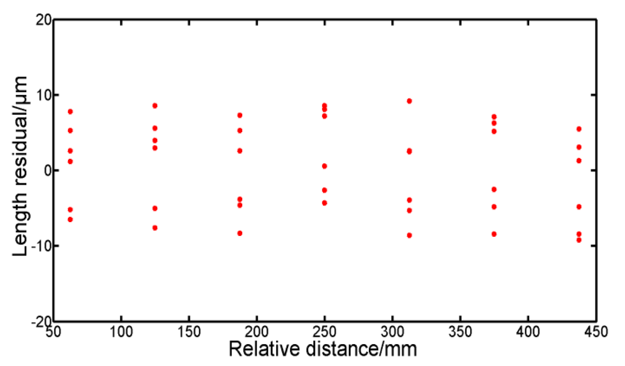
Figure 10.
Comparison of the measured root mean square error with the CRLB.

© 2018 by the authors. Licensee MDPI, Basel, Switzerland. This article is an open access article distributed under the terms and conditions of the Creative Commons Attribution (CC BY) license (http://creativecommons.org/licenses/by/4.0/).
Share and Cite
MDPI and ACS Style
Xiong, X.-T.; Qu, X.-H.; Zhang, F.-M. Error Correction for FSI-Based System without Cooperative Target Using an Adaptive Filtering Method and a Phase-Matching Mosaic Algorithm. Appl. Sci. 2018, 8, 1954. https://doi.org/10.3390/app8101954
AMA Style
Xiong X-T, Qu X-H, Zhang F-M. Error Correction for FSI-Based System without Cooperative Target Using an Adaptive Filtering Method and a Phase-Matching Mosaic Algorithm. Applied Sciences. 2018; 8(10):1954. https://doi.org/10.3390/app8101954
Chicago/Turabian StyleXiong, Xing-Ting, Xing-Hua Qu, and Fu-Min Zhang. 2018. "Error Correction for FSI-Based System without Cooperative Target Using an Adaptive Filtering Method and a Phase-Matching Mosaic Algorithm" Applied Sciences 8, no. 10: 1954. https://doi.org/10.3390/app8101954
Note that from the first issue of 2016, this journal uses article numbers instead of page numbers. See further details here.