Detection of Ventricular Fibrillation Using the Image from Time-Frequency Representation and Combined Classifiers without Feature Extraction

Abstract

Due the fact that the required therapy to treat Ventricular Fibrillation ($VF$) is aggressive (electric shock), the lack of a proper detection and recovering therapy could cause serious injuries to the patient or trigger a ventricular fibrillation, or even death. This work describes the development of an automatic diagnostic system for the detection of the occurrence of $VF$ in real time by means of the time-frequency representation ($TFR$) image of the ECG. The main novelties are the use of the $TFR$ image as input for a classification process, as well as the use of combined classifiers. The feature extraction stage is eliminated and, together with the use of specialized binary classifiers, this method improves the results of the classification. To verify the validity of the method, four different classifiers in different combinations are used: Regression Logistic with L2 Regularization ($L2RLR$), adaptive neural network ($ANNC$), Bagging ($BAGG$), and K-nearest neighbor ($KNN$). The Hierarchical Method (HM) and Voting Majority Method (VMM) combinations are used. ECG signals used for evaluation were obtained from the standard MIT-BIH and AHA databases. When the classifiers were combined, it was observed that the combination of $BAGG$, $KNN$, and $ANNC$ using the Hierarchical Method (HM) gave the best results, with a sensitivity of 95.58 ± 0.41%, a 99.31 ± 0.08% specificity, a 98.6 ± 0.04% of overall accuracy, and a precision of 98.25 ± 0.29% for $VF$. Whereas a sensitivity of 94.02 ± 0.58%, a specificity of 99.31 ± 0.08%, an overall accuracy of 99.14 ± 0.43%, and a precision of 98.59 ± 0.09% was obtained for $VT$ with a run time between 0.07 s and 0.12 s. Results show that the use of $TFR$ image data to feed the combined classifiers yields a reduction in execution time with performance values above to those obtained by individual classifiers. This is of special utility for $VF$ detection in real time.

1. Introduction

The most common causes of sudden death are cardiovascular diseases, which are among the leading causes of death worldwide. One of the cardiovascular diseases with the highest mortality is Ventricular Fibrillation ($VF$), which is a cardiac arrhythmia condition produced by a disorganized electrical activity in the ventricles. During $VF$, the ventricles contract with an absence of an effective beat causing a pumping failure which could lead to a sudden death if the patient is not adequately treated within a few minutes. Defibrillation is the only definitive treatment for $VF$. It consists of applying a high voltage electric shock on the patient’s chest, facilitating the restart of a normal electrical cardiac activity [1,2,3]. However, the success of defibrillation is inversely proportional to the interval of time lapsed from the beginning of the episode to the application of the discharge.

There are many difficulties in diagnosing $VF$: On the one hand, the intrinsic characteristics of the $VF$ signal (lack of organization, irregularity, etc.) and, on the other hand, the great similarity between VF and other cardiac pathologies such as ventricular tachycardia ($VT$) [4], especially in early stages of $VF$. The differentiation between $VT$ and $VF$ is quite complex: The wrongful diagnosis of $VF$ for a patient that really suffers of $VT$ can cause serious complications at the time of applying the therapy corresponding to $VF$ (high voltage electrical discharge), as it may cause $VF$ to the patient. On the contrary, if $VF$ is incorrectly interpreted as $VT$ or any other cardiac rhythm, the result can also be dangerous for the patient’s life since the treatment would imply receiving less voltage than the appropriate level. Thus, an effective detection method for distinguishing $VF$ from $VT$ is critical in clinical research.

The electrocardiogram (ECG) is a non-invasive, low-cost examination tool that has been used as the basic method of diagnosing cardiac conduction disorders by studying the heart rate and morphology of different waves that constitute the cardiac cycle. ECG analysis is a good source of information from which different types of heart disease can be detected. Due to the fact that the ECG signal is a non-stationary random signal, the time domain analysis does not prove to be sufficiently sensitive to the distortions of the ECG waveforms. However, these methods do not always show all the information that can be extracted from the ECG signals [5,6], thus losing information on the frequency domain which shows additional information on the signal.

Diagnosis in the frequency domain [7] uses methods such as the Fourier transform. Therefore, the analysis in the frequency domain allows to determine the frequencies of the signal. On the other hand, the temporary-type information of the signal is lost, which is a very limited method and is not useful for the analysis of non-stationary signals. Several studies have used mathematical models that combine temporal and spectral information in the same representation. 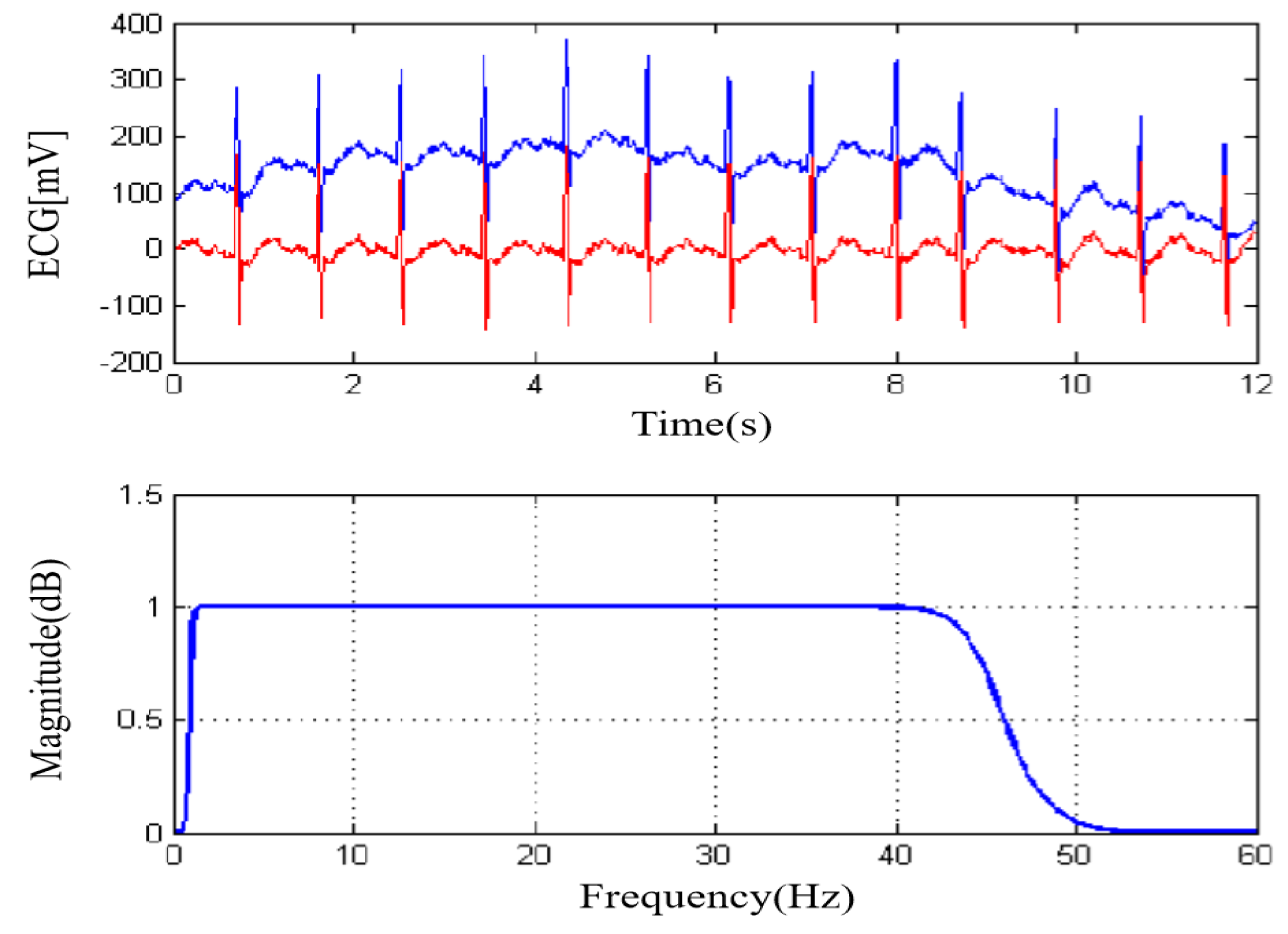This technique of Time-Frequency Representation ($TFR$) is very important in the treatment of non-stationary signals such as the ECG signal, as it distributes the energy of the signal in a two-dimensional time-frequency space [8,9]. In addition, multiple factors might alter the acquisition and recording of the ECG signal: The influence of the environment, 50–60 Hz mains interference, variations of the base line of low-frequency interference in the range of 0 Hz to 0.5 Hz [10,11]. On the other hand, there are disturbances of physiological origin such as those of electromyography (EMG). ECG noise reduction has been one of the main fields of research in the last decades since an adequate noise reduction allows a good pre-processing of the signal, extracting the maximum amount of information possible and eliminating ECG signal contamination from other sources.

Usually, after the initial processing of the signal, several algorithms are applied to obtain characteristics, features, or parameters which are supposed to offer a difference in value depending on the pathology. Typically, these parameters can be redundant or remove relevant information, being necessary to apply different techniques to select the most adequate. After optimisation, selected parameters are intended to serve as input to a classifier responsible for separating classes (associated to a pathology or type of rhythm, in this case), i.e. identified signal types.

In order to improve the performance of individual classifiers, the combination of classifiers (multiclassifiers) can improve the performance in separating classes. It is based on constructing a global classifier built from a set of classifiers that can provide interesting information on the representation of data compared to the results achieved using individual classifiers. There are many examples in the literature that have used the combination of classifiers focused towards the field of bioinformatics and biomedical research, geophysical analysis and remote sensing, among others. Out of the most frequently used multi classifiers, Random Forests [12], Bagging [8], Boosting [13], or Random Subspaces are the most commonly employed multiclassifiers. In the case of Random Subspaces, different subsets of attributes are used to train each individual classifier. The Bagging type variety comes from using different subsets of instances to train each individual classifier. Random Forests is a substantial modification of bagging that uses Random Trees as individual classifiers. The Boosting type iteratively trains the individual classifiers, therefore, it modifies the weights of the instances that will use the next individual classifier. There are other methods such as cascading [14], Stacking [15], and Grading [16].

Other examples using a combination of classifiers for ECG signal analysis can be found in the literature as a multiple classifier system [17], a genetic ensembles of classifiers [18], or a classification approach that uses majority voting optimized by the taguchi method [19]. In some cases, a majority voting [20,21], or a combined stacking technique [22]. Other combinations are also applied, e.g., an application of the decision tree to integrate the results of a set of individual neural classifiers (MLP, TSK, and the SVM) working in parallel [23] or a majority voter determining the P-wave absence over seven beats [24].

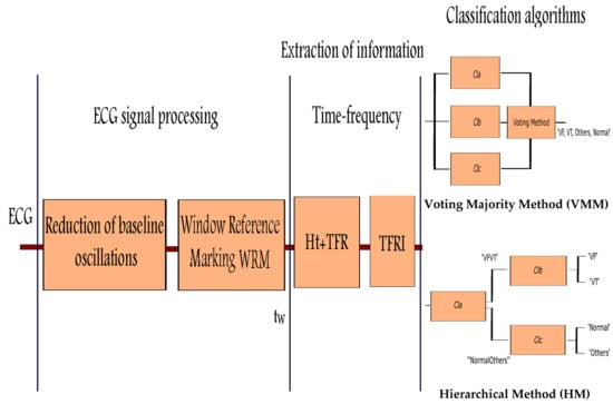
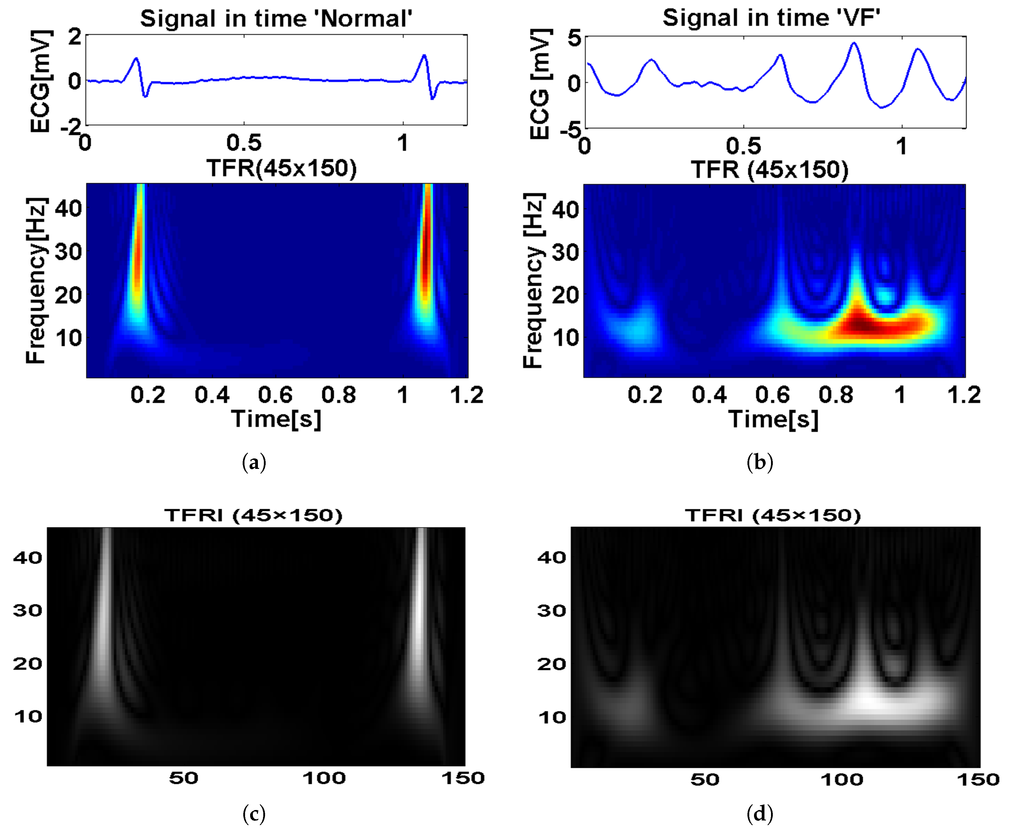
This work proposes a new strategy for the detection of $VF$ whose steps are the initial processing of the signal and obtaining its time-frequency representation ($TFR$) with its equivalent image ($TFRI$). The $TFR$ or $TFRI$ (both cases will be analysed) is directly entered into an individual classifier or combined, without calculating parameters or extracting features since time-frequency representation contains both temporal and spectral information from the ECG signal, allowing the classifier to have enough information for the detection of different types of cardiac pathologies in real time. Since the ECG is a temporal signal, it is not common to find works converting the temporal signal into an image and further analyse the image, some works used some geometrical features from the ECG in combination with other features entering the classification stage. Other works also extract features from a time-frequency or discrete wavelet transform, but they do not use it as an image.

In order to reach the objectives sought, the present work is structured as follows: Section 2 describes the materials and methods, followed by Section 3 which details the initial processing applied to the ECG signal. Section 4 shows the extraction of information. Section 5 presents the individual and combined classification algorithms. Section 6 shows the standard statistical indexes, and finally, Section 7 shows obtained results for individual and combined classifiers, and Section 8 and Section 9 give a comparison of results with other authors and conclusions, respectively.

2. Materials and Methods

Records of the ECG signals have been taken from the standard MIT-BIH Malignant Ventricular Arrhythmia Database [25,26] and AHA (2000 series) [27], generating both the training and the test sets from them. In total, 24 continuous monitoring records (22 MIT-BIH records plus two additional AHA records) were used, with a sampling frequency of 125 Hz. All records have cardiac events already labeled. The additional AHA records aim to increase the number of Ventricular Tachycardia ($VT$) episodes to improve the balance between recorded time of $VT$ and $VF$ episodes. With the episodes labeled, four groups (classes) of signals were created: Ventricular Fibrillation ($VF$) corresponds to the class $VF$ represents all the sections of registers in which there has been ventricular fibrillation and ventricular flutter. ECG signals with the presence of ventricular tachycardia were assigned to the class $VT$, which, in many cases, appear as a prior stage to ventricular fibrillation (sometimes, $VT$ sections have $VF$-like morphologies). Normal rhythms were assigned to the $Normal$ class that constitutes the segments labeled with sinus rhythm. Finally, the rest of signal types not labelled as the previous classes (other arrhythmias, noise, etc.) have also been considered and assigned to the class $Others$. In total, 20,040 s were generated for all ECG signal registers, 3600 s corresponded to the class $VF$, 1380 s to $VT$, 10,860 s to $Normal$, and 4200 s to $Others$.

3. ECG Signal Processing

If we look for a classifier that can obtain a satisfactory result of detecting $VF$ and its differentiation from $VT$, it is necessary that the data provided as input to this classifier are properly treated. For this reason, different stages of data conditioning are performed to both the temporal signal of ECG and its time-frequency representation $TFR$. Figure 1 shows the general scheme of the followed methodology, from the reading of the records of the database to the results obtained by the classifier.

The developed methodology is composed of three fundamental phases.

• First phase: Data filtering in order to reduce the baseline that affects the ECG. Once filtered, obtain the Window Reference Mark ($WRM$) of the ECG signal. Each $WRM$ indicates the beginning of a time window ($t_w$) of the ECG signal.
• Second phase: Extraction of information through the implementation of the Hilbert transform to each window $t_w$ obtained in the first phase, then, assesment of the $TFR$ matrix using the Pseudo Wigner-Ville, and the Time-Frequency Representation Image ($TFRI$).
• Third phase: The classification phase is carried out considering both the individual and combined classifiers used. In this phase, the previously obtained $TFRI$ matrices are used as input. The success in the detection of $VF$ depends on the processing of the signal and the structure of the classifiers used. In order to better adapt to the data, we must adjust the parameters of the classifier to obtain the best performance.

3.1. Reduction of Baseline Oscillations

The first step in the processing of the ECG signal is to use a baseline filter, reducing the variation of the baseline and thus obtaining a better quality and definition of the temporal signal that will result in better characteristics provided by the $TFR$. This processing consists of the implementation of an 8th order infinite impulse response filter (IIR) with a Butterworth bandpass type ranging from 1 Hz to 45 Hz [28,29]. Figure 2 represents the effect of applying this bandpass filter, showing a reduction of the baseline. Thus, all signal contribution not located in the mentioned frequency range, which corresponds to non-ECG source, are eliminated.

3.2. Reference Marks

Next, it is necessary to obtain a Window Reference Mark ($WRM$) to indicate the beginning of the $t_w$ ECG time window. Following [30], a value from 50 to 120 beats per minute (bpm) can be considered as a normal heart rate range, and thus, the minimum ($WR{M}_{min}$) and the maximum ($WR{M}_{max}$) distances between two consecutive $WRM$ is 0.5 s and 1.2 s, respectively. Accordingly, these values were used in our analysis. The calculation of $WRM$ reference marks was obtained by an already developed algorithm [8], where $N_{LMC}$ is the number of local maxima $LM$ marks existing in the signal. From each previously generated $WRM$ reference mark, a time window $t_w$ of 1.2 s in length (150 samples) was generated, starting at the corresponding $WRM$ mark, $t_w$ = [$WRM$, $WRM+1.2$ s] as shown in (Equation (1)).

$$\begin{array}{c}\hfill t{w}_j=[WR{M}_j,WR{M}_j+1.2\mathrm{s}];j=1,...,N_{LMC}\end{array}$$

(1)

4. Extraction of Information

For each window $t_w$, the Hilbert transform (Ht) is calculated first and then $TFR$ of the PWV (Pseudo Wigner-Ville) type is calculated. Once the $TFR$ is obtained, the contributions of frequency over 45 Hz are canceled, thereby eliminating both the network interference (50 Hz or 60 Hz) as well as the electromyogram (EMG). After this process, a Data Matrix ($D{M}^{{}^{\prime }}$) obtained from the $TFR$, being $45\times 150$ in size is obtained. This is useful since the signal of interest is found in values below 45 Hz (see Figure 3a,b).

Once $D{M}^{{}^{\prime }}$ is obtained from the $TFR$ for each $t_w$ window, this data matrix $TFR$ is converted into an image $TFR{I}_{L_f\times L_t}$ with size $L_f\times L_t$ pixels being $L_f=45$ and $L_t=150$ converting the energy levels of the signal into a pixel intensity range from 0 to 255. These values correspond to different levels of grey in an image as they are shown in Figure 3c,d. Each $TFRI$ image is then stored in a Data Matrix ($D{M}^{{}^{″}}$) of size $45\times 150$.

Once $D{M}^{{}^{″}}$ data matrix is obtained, the data matrix is directly fed into the classifier. By doing this, all ECG signal information in the temporal and spectral domains is contained in the data matrix, providing the classifier with maximal data information. Note that this method requires a large number of inputs to the classifiers ($45\times 150=6750$) since each $D{M}_{ij}^{{}^{″}}$ data in a matrix coordinate corresponds to an input. It is important to note that there is no feature extraction from the data matrix $D{M}^{{}^{″}}$ as it contains the temporal and spectral information from the ECG signal.

5. Classification Algorithms

In this work, several classifiers are used to evaluate the efficiency of the $VF$ detection algorithm. All $D{M}^{{}^{″}}$ data were separated into two subsets: One for training and one for test. The training subset is used so that the algorithms learn to discriminate among the various types of defined classes ($VF$, $VT$, $Normal$, and $Others$). As soon as each classifier concludes its training, it generates a prediction function that is later used to evaluate new data. Each of the classifiers used in this work have parameters that must be optimized for the purpose of obtaining the maximum yield. The tuning of the classifiers is done on the basis of final classification performance.

Some algorithms propose the use of four classes [8,31]. However, we can combine different binary algorithms for two-class separation so that they can provide important complementary information about the representation of the data.

Combination Topologies

The parallel topology method is the most frequent in combination of classifiers. All the classifiers are run in parallel using the same input data, and the results achieved by all the classifiers (classifier1-$Cla$, classifier2-$Clb$, classifier3-$Clc$) generate a multiclassifier result ($Cla\_Clb\_Clc$) that are combined with the objective of obtaining an appropriate decision using a combination rule, e.g., the voting method [32], as shown in Figure 4 which is called Voting Majority Method (VMM). For real time execution, this methodology has a high execution time since all classification algorithms must be executed to make the final decision. The voting method works in the same way as the humans when voting in political elections. In other words, depending on the number of votes reached in favor of each class, it is assigned to the one that obtains the majority.

In a hierarchical topology, parallel and cascaded topologies are combined (Figure 5). By joining these two approaches, better results than those achieved by using individual classifiers can be obtained. The first classifier ($Cla$) generates a binary output for signal to be $VFVT$ or $NormalOthers$. Then, two specific classifiers $Clb$ and $Clc$ generate a new binary classification $VF$, $VT$ for the signal classified as $VFVT$ by $Cla$, and $Others$, $Normal$ for the signal classified as $NormalOthers$, respectively. By joining the classifiers, a multi-class cascaded algorithm is generated.

6. Performance Assessment

To evaluate the performance of the classifier, we use standard statistical indexes such as Sensitivity (Sens), Specificity (Spe), Accuracy (Acc), and Precision (Pre), as shown by Equations (2)–(5), where TP are the True Positives, FN the False Negatives, TN the True Negatives, and FP the False Positives [33].

$$\begin{array}{c}\hfill Sensitivity(\%)=\frac{TP}{TP+FN}\times 100\end{array}$$

(2)

$$\begin{array}{c}\hfill Specificity(\%)=\frac{TN}{TN+FP}\times 100\end{array}$$

(3)

$$\begin{array}{c}\hfill Accuracy(\%)=\frac{TP+TN}{TP+FN+TN+FP}\times 100\end{array}$$

(4)

$$\begin{array}{c}\hfill Precision(\%)=\frac{TP}{TP+FP}\times 100\end{array}$$

(5)

The calculation of the value of the global specificity, accuracy and Precision of one of the types ($VF$, $VT$, $Normal$, $Others$) is obtained by using the specificity, accuracy, and Precision of this type of pathology before the sum of the remaining pathology types. The execution time of each of the tests performed was measured using a Fujitsu AH544 (Tokyo, Japan) laptop computer with an Intel (R) Core (TM) [email protected] GHz processor with 8GB RAM, 64-bit operating system using Matlab (R).

For completion, the Receiver Operating Characteristic (ROC) curve and Area Under the Curve (AUC) values are also calculated.

7. Results

In total, 28,507 windows were generated for all $M{D}^{{}^{″}}$ obtained from the corresponding $TFRI$: 5309 corresponded to the class $VF$, 1987 to $VT$, 15,160 to $Normal$, and 6051 to $Others$. For each class, 67% of the data were used for training, and the rest for testing. This approach is repeated by making a 5-fold cross validation: Individual and combined classifier algorithms are assessed by taking the average of these 5 iterations. A 5-fold validation was chosen amongst different z-fold possibilities after some trials, with 5-fold cross validation obtaining the lowest generalization error, thus minimizing the structural risk of classifiers. For 5-fold cross validation, each class was divided into five datasets, equal in size; four dataset were used for training and one for testing. After five iterations, all datasets served for training and testing, obtaining a more balanced result.

Different analyses were done, the first test is based on different types of individual classification algorithms, the second uses combined classification algorithms.

7.1. Results for Individual Classifiers

In this first test, individual classifiers are used. The results are obtained using four different classification algorithms: $L2RLR$, $ANNC$, $BAGG$, and $KNN$ [8,31]. After several trials, the parameters for the classifiers were the following:

• $L2RLR$: With regularization parameter $\lambda ={10}^{-9}$. In this case, the $\lambda$ value is very small to account for high values in regression coefficients.
• $ANNC$: Two hidden layers, 20 neurons in each hidden layer. Two layers allow better classification in case of a high number of inputs, as in this case. In case of a single layer, a higher number of neurons should be used.
• $BAGG$: 600 decision trees. This was an experimental value. A higher number of trees did not produce better results.
• $KNN$: Euclidean distance showed a good performance, together with K = 1.

Table 1. Results for the different algorithms adaptive neural network ($ANNC$), Bagging ($BAGG$), L2 Regularization ($L2RLR$), and K-nearest neighbor ($KNN$) using as input the time-frequency representation image ($TFRI$) used to characterize and detect $VF$ and $VT$ classes.

Class	VF				VT
	Sens %	Spe %	Acc %	Pre %	Sens %	Spe %	Acc %	Pre %
Classification Algorithms	VF	Global	Global	Global	VT	Global	Global	Global
$L2RLR$
Test	91.54 ± 0.46	98.45 ± 0.06	97.15 ± 0.09	94.74 ± 1.27	88.15 ± 0.59	98.81 ± 0.04	98.07 ± 0.07	89.67 ± 1.77
$ANNC$
Test	95.56 ± 0.33	98.80 ± 0.13	98.19 ± 0.15	95.26 ± 0.45	88.80 ± 1.13	99.52 ± 0.06	98.87 ± 0.03	94.05 ± 0.80
$BAGG$
Test	98.46 ± 0.26	98.43 ± 0.12	98.44 ± 0.14	97.09 ± 0.14	84.8 ± 1.70	99.86 ± 0.04	98.82 ± 0,12	97.81 ± 0.82
$KNN$
Test	94.97 ± 0.70	99.27 ± 0.05	98.47 ± 0.01	97.09 ± 0.14	93.47 ± 0.19	99.39 ± 0.15	98.97 ± 0.08	92.11 ± 0.70

and

Table 2. Results for individual algorithms $ANNC$, $BAGG$, $L2RLR$, and $KNN$ using as input the $TFRI$ used to characterize and detect $Others$ and $Normal$ classes.

Class	Others				Normal
	Sens %	Spe %	Acc %	Pre %	Sens %	Spe %	Acc %	Pre %
Classification Algorithms	Others	Global	Global	Global	Normal	Global	Global	Global
$L2RLR$
Test	94.80 ± 0.55	98.79 ± 0.03	97.91 ± 0.12	96.29 ± 0.98	97.63 ± 0.12	96.61 ± 0.4	97.17 ± 0.27	97.56 ± 0.68
$ANNC$
Test	96.87 ± 1.06	99.55 ± 0.08	98.96 ± 0.21	98.45 ± 0.39	98.98 ± 0.13	97.72 ± 0.56	98.40 ± 0.27	98.39 ± 0.22
$BAGG$
Test	95.66 ± 0.31	99.87 ± 0.02	98.95 ± 0.07	99.60 ± 0.10	99.39 ± 0.19	97.61 ± 0.09	98.57 ± 1.31	97.71 ± 0.04
$KNN$
Test	97.69 ± 0.21	99.40 ± 0.04	99.03 ± 0.05	97.92 ± 0.16	99.07 ± 0.08	98.29 ± 0.10	98.71 ± 0.06	98.66 ± 0.06

summarize the results achieved by making comparisons between the values of sensitivity, specificity, accuracy, and precision. When analyzing the values shown in the tables, it is observed that the $KNN$ classifier obtained the best result, with a sensitivity of 94.97 ± 0.70%, a global specificity of 99.27 ± 0.05%, accuracy of 98.47 ± 0.01%, and an overall precision of 97.09 ± 0.14% achieved for $VF$. For $VT$, a sensitivity of 93.47 ± 0.19%, specificity of 99.39 ± 0.15%, accuracy 98.97 ± 0.08%, and an overall precision of 92.11 ± 0.7% was obtained.

For a complete analysis, the confusion matrices for the classes and the used algorithms were calculated (

Table 3. Confusion matrix for classification of $VF$, $VT$, $Others$, and $Normal$ using the $L2RLR$ and $ANNC$ algorithms.

Algorithms	L2RLR				ANNC
	VF	VT	Others	Normal	VF	VT	Others	Normal
$VF$	1627	64	13	48	1689	34	3	26
$VT$	59	583	2	12	55	589	0	12
$Others$	9	0	1909	79	11	1	1941	44
$Normal$	32	8	68	4895	18	3	27	4955

and

Table 4. Confusion matrix for classification of $VF$, $VT$, $Others$, and $Normal$ using the $BAGG$ and $KNN$ algorithms.

Algorithms	BAGG				KNN
	VF	VT	Others	Normal	VF	VT	Others	Normal
$VF$	1721	9	2	20	1666	52	13	21
$VT$	85	564	0	7	27	618	0	11
$Others$	4	1	1902	90	8	0	1954	35
$Normal$	16	3	6	4978	14	1	29	4949

). These tables show that the main conflicts exist in pairs: $VF$ and $VT$, $Normal$ and $Others$. Actually, since the number of segments is lower for $VF$ and $VT$ compared to normal and Others, the proportion of confusion mainly resides in $VF$ and $VT$S, which was expected according to other algorithm results and clinical practice.

Comparing the results offered by the different algorithms, there is an important variation in the results for the sensitivities of $VF$ and $VT$ depending on the algorithm. For instance, if the sensitivity level for $VF$ is high, the sensitivity for $VT$ decreases. It can be observed that the $KNN$ classifier achieves the best performance for the proposed methodology due to the adequate detection and discrimination capacity of $VF$ when compared against the rest of classes. However, it has a high execution time because the $KNN$ algorithm requires many iterations to calculate the closest distances. For the $ANNC$ algorithm, the classes are separated by means of a surface that maximizes the margin among them, with the least number of training errors, having a computational cost much lower than that obtained with $KNN$. The $L2RLR$ algorithm has less time of execution because it is based on probabilities. The Bagging creates its individual classifiers by training a system of classification on different bootstrap samples of the training set, thus retrieving a higher run time than the rest of the classifiers (except for $KNN$).

7.2. Comparative Study for the Method of Combined Classifiers

In this section, the results obtained by the combination methods are described: Voting Majority Method (VMM) and Hierarchical Method (HM) described above. In the classification tests performed, we show how the combination of classification algorithms behaves in relation to the results obtained in the previous test using individual classifiers. For proper comparison, the same $D{M}^{{}^{″}}$ data used for individual classifiers, and the same classifier parameters were used in these analyses.

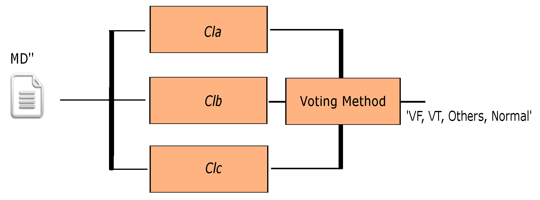
In the first analysis, the Voting Majority Method (VMM) is applied using different combinations of three individual classification algorithms in parallel, the results obtained are shown in

Table 5. Results for the voting majority method (VMM) combination method using $TFRI$ as data input. Results correspond to detection of $VF$ and $VT$ pathologies.

Class	VF				VT
	Sens %	Spe %	Acc %	Pre %	Sens %	Spe %	Acc %	Pre %
Combined Classification Algorithms (Cla,Clb,Clc)	VF	Global	Global	Global	VT	Global	Global	Global
$ANNC\_KNN\_L2RLR$
Test	97.47 ± 0.13	99.09 ± 0.10	98.71 ± 0.06	96.12 ± 0.23	91.31 ± 0.88	99.97 ± 0.08	99.18 ± 0.01	96.26 ± 0.90
$ANNC\_KNN\_BAGG$
Test	98.46 ± 0.06	98.98 ± 0.02	98.89 ± 0.01	96.04 ± 0.60	89.63 ± 0.30	99.86 ± 0.01	99.14 ± 0.02	97.64 ± 0.15
$BAGG\_KNN\_L2RLR$
Test	98.43 ± 0.16	98.98 ± 0.08	98.87 ± 0.04	95.79 ± 0.50	91.01 ± 0.68	99.83 ± 0.03	99.16 ± 0.02	97.51 ± 0.18
$BAGG\_ANNC\_L2RLR$
Test	97.89 ± 0.08	98.84 ± 0.05	98.66 ± 0.04	95.33 ± 0.31	87.80 ± 1.21	99.88 ± 0.03	99.98 ± 0.06	97.61 ± 0.50

,

Table 6. Results for the VMM combination method using $TFRI$ as data input. Results correspond to detection of $Other$ and $Normal$ classes.

Class	Others				Normal
	Sens %	Spe %	Acc %	Pre %	Sens %	Spe %	Acc %	Pre %
Combined Classification Algorithms (Cla,Clb,Clc)	Others	Global	Global	Global	Normal	Global	Global	Global
$ANNC\_KNN\_L2RLR$
Test	97.35 ± 0.15	99.67 ± 0.02	99.16 ± 0.03	98.57 ± 0.05	99.22 ± 0.05	98.41 ± 0.09	98.84 ± 0.03	98.63 ± 0.02
$ANNC\_KNN\_BAGG$
Test	97.20 ± 0.11	99.84 ± 0.04	99.27 ± 0.01	99.21 ± 0.14	99.52 ± 0.06	98.29 ± 0.05	98.95 ± 0.01	98.64 ± 0.04
$BAGG\_KNN\_L2RLR$
Test	96.95 ± 0.11	99.77 ± 0.04	99.16 ± 0.01	99.25 ± 0.18	99.4 ± 0.05	98.30 ± 0.03	98.89 ± 0.01	98.51 ± 0.02
$BAGG\_ANNC\_L2RLR$
Test	96.54 ± 0.09	99.74 ± 0.05	99.05 ± 0.02	99.12 ± 0.17	99.38 ± 0.09	97.68 ± 0.23	98.59 ± 0.09	98.26 ± 0.17

,

Table 7. Confusion matrix for classification of $VF$, $VT$, $Others$, and $Normal$ classes using the $ANNC\_KNN\_L2RLR$ and $ANNC\_KNN\_BAGG$ VMM combined classifier.

Algorithms	$\mathit{ANNC}\_\mathit{KNN}\_\mathit{L}2\mathit{RLR}$				$\mathit{ANNC}\_\mathit{KNN}\_\mathit{BAGG}$
	VF	VT	Others	Normal	VF	VT	Others	Normal
$VF$	1706	23	5	18	1720	17	2	13
$VT$	45	600	1	10	53	595	0	8
$Others$	8	0	1948	41	6	1	1943	47
$Normal$	14	0	23	4965	14	1	15	4973

and

Table 8. Confusion matrix for classification of $VF$, $VT$, $Others$, and $Normal$ classes using the $BAGG\_KNN\_L2RLR$ and $BAGG\_ANNC\_L2RLR$ VMM combined classifier.

Algorithms	$\mathit{BAGG}\_\mathit{KNN}\_\mathit{L}2\mathit{RLR}$				$\mathit{BAGG}\_\mathit{ANNC}\_\mathit{L}2\mathit{RLR}$
	VF	VT	Others	Normal	VF	VT	Others	Normal
$VF$	1724	14	0	14	1717	13	2
$VT$	55	595	0	6	62	586	0	8
$Others$	6	1	1935	55	7	0	1930	60
$Normal$	14	1	14	4974	15	1	16	4971

. When analyzing the results from the tables, it can be seen, in both cases, that the detection of $VF$ has significantly improved when compared with individual classifiers. However, the detection of $VT$ has decreased when compared with what those obtained by the $KNN$ algorithm, which was the best individual classifier. It is concluded that the combination of classifiers do not exceed the results obtained in case of $KNN$.

In the second analysis, the Hierarchical Method (HM) is applied to three individual algorithms ($Cla$, $Clb$, $Clc$) getting the $Cla\_Clb\_Clc$ multiclassifier where $Clb$ and $Clc$ are in parallel and both cascaded after $Cla$ (Figure 5). The obtained results are shown in

Table 9. Results for different hierarchical method (HM) combined classifier methods to detect $VF$ and $VT$ pathologies.

Class	VF				VT
	Sens %	Spe %	Acc %	Pre %	Sens %	Spe %	Acc %	Pre %
Combined Classification Algorithms (Cla,Clb,Clc)	VF	Global	Global	Global	VT	Global	Global	Global
$ANNC\_KNN\_ANNC$
Test	95.13 ± 0.06	99.10 ± 0.04	98.41 ± 0.04	96.38 ± 0.19	92.32 ± 0.66	99.33 ± 0.07	98.91 ± 0.02	91.38 ± 0.84
$ANNC\_KNN\_L2RLR$
Test	94.89 ± 0.56	99.08 ± 0.20	98.32 ± 0.27	96.02 ± 0.87	92.37 ± 2.46	99.27 ± 0.10	98.78 ± 0.23	90.71 ± 1.38
$BAGG\_KNN\_ANNC$
Test	95.58 ± 0.40	99.31 ± 0.08	98.6 ± 0.04	98.25 ± 0.29	94.02 ± 0.58	99.31 ± 0.08	99.14 ± 0.43	98.59 ± 0.09
$BAGG\_KNN\_L2RLR$
Test	95.58 ± 0.42	99.31 ± 0.04	98.6 ± 0.05	96.93 ± 0.19	94.02 ± 0.58	99.31 ± 0.08	99.14 ± 0.43	91.25 ± 0.91
$L2RLR\_KNN\_ANNC$
Test	93.33 ± 0.31	98.93 ± 0.07	97.88 ± 0.12	95.30 ± 0.96	92.01 ± 0.58	99.22 ± 0.09	98.71 ± 0.03	90.06 ± 1.37
$L2RLR\_KNN\_L2RLR$
Test	93.54 ± 0.31	98.01 ± 0.07	97.98 ± 0.12	95.65 ± 0.35	92.95 ± 0.58	99.26 ± 0.08	98.82 ± 0.03	90.70 ± 0.98

and

Table 10. Results for different HM combined classifier methods to detect $Normal$ and $Others$ classes.

Class	Others				Normal
	Sens %	Spe %	Acc %	Pre %	Sens %	Spe %	Acc %	Pre %
Combined Classification Algorithms (Cla,Clb,Clc)	Others	Global	Global	Global	Normal	Global	Global	Global
$ANNC\_KNN\_ANNC$
Test	97.22 ± 0.14	99.57 ± 0.11	99.06 ± 0.10	98.45 ± 0.39	99.04 ± 0.15	98.10 ± 0.26	98.61 ± 0.15	98.39 ± 0.22
$ANNC\_KNN\_L2RLR$
Test	96.11 ± 0.67	99.18 ± 0.33	98.45 ± 0.38	96.70 ± 1.16	98.42 ± 0.43	97.67 ± 0.26	98.17 ± 0.30	98.01 ± 0.22
$BAGG\_KNN\_ANNC$
Test	97.42 ± 0.12	99.52 ± 0.07	99.07 ± 0.08	98.25 ± 0.29	99.02 ± 0.14	98.36 ± 0.10	98.72 ± 0.11	98.59 ± 0.09
$BAGG\_KNN\_L2RLR$
Test	96.92 ± 0.38	98.92 ± 0.05	98.28 ± 0.04	96.10 ± 0.17	98.22 ± 0.07	97.73 ± 0.19	97.99 ± 0.05	98.06 ± 0.16
$L2RLR\_KNN\_ANNC$
Test	97.22 ± 0.11	99.50 ± 0.06	99.01 ± 0.07	98.20 ± 0.24	98.61 ± 0.14	97.39 ± 0.27	98.05 ± 0.18	97.79 ± 0.23
$L2RLR\_KNN\_L2RLR$
Test	95.71 ± 0.30	98.84 ± 0.02	98.16 ± 0.04	95.83 ± 0.07	97.81 ± 0.08	96.89 ± 0.32	97.38 ± 0.10	97.34 ± 0.27

with confusion matrices in

Table 11. Confusion matrix for classification of $VF$, $VT$, $Others$, and $Normal$ using the $ANNC\_KNN\_ANNC$ and $ANNC\_KNN\_L2RLR$ combined classifiers in HM topolgy.

Algorithms	$\mathit{ANNC}\_\mathit{KNN}\_\mathit{ANNC}$				$\mathit{ANNC}\_\mathit{KNN}\_\mathit{L}2\mathit{RLR}$
	VF	VT	Others	Normal	VF	VT	Others	Normal
$VF$	1667	56	3	26	1662	60	7	23
$VT$	33	612	0	11	38	606	1	11
$Others$	12	0	1941	44	12	0	1919	66
$Normal$	19	2	27	4955	18	2	59	4924

,

Table 12. Confusion matrix for classification of $VF$, $VT$, $Others$, and $Normal$ using the $BAGG\_KNN\_ANNC$ and $BAGG\_KNN\_L2RLR$ combined classifiers in HM topolgy.

Algorithms	$\mathit{BAGG}\_\mathit{KNN}\_\mathit{ANNC}$				$\mathit{BAGG}\_\mathit{KNN}\_\mathit{L}2\mathit{RLR}$
	VF	VT	Others	Normal	VF	VT	Others	Normal
$VF$	1674	56	5	17	1674	56	7	15
$VT$	32	617	0	7	32	617	1	6
$Others$	5	0	1945	47	5	0	1916	76
$Normal$	16	3	30	4954	16	3	70	4914

and

Table 13. Confusion matrix for classification of $VF$, $VT$, $Others$, and $Normal$ using the $L2RLR\_KNN\_ANNC$ and $L2RLR\_KNN\_L2RLR$ combined classifiers in HM topolgy.

Algorithms	$\mathit{L}2\mathit{RLR}\_\mathit{KNN}\_\mathit{ANNC}$				$\mathit{L}2\mathit{RLR}\_\mathit{KNN}\_\mathit{L}2\mathit{RLR}$
	VF	VT	Others	Normal	VF	VT	Others	Normal
$VF$	1635	60	6	51	1639	56	12	45
$VT$	38	604	0	14	32	610	1	13
$Others$	9	0	1941	47	9	1	1911	76
$Normal$	32	7	30	4934	33	7	69	4894

.

Since $KNN$ was the best individual algorithm in the detection and discrimination between $VF$ and $VT$, it was chosen as $Clb$. The $ANNC$, $BAGG$, $L2RLR$ algorithms are taken as $Cla$ for the discrimination between the classes $VFVT$ and $NormalOthers$ and the $ANNC$ and $L2RLR$ algorithms are used as $Clc$ for $Normal$ and $Others$ discrimination. Analyzing the results, it can be concluded that the combinational algorithms have a similar or better behavior than the individual $KNN$ in the detection of $VF$ in very large datasets and high dimensionality, with a reduced execution time.

With all the results obtained, the use of combined algorithms can be recommended as the best method of classification. In addition, results obtained using the combination $BAGG\_KNN\_ANNC$ using HM showed better classification ratio when compared to those obtained using the algorithms individually, and other multi classifiers.

The $BAGG\_KNN\_ANNC$ HM obtained a good behavior in the discrimination between the classes $VF$, $VT$, $Normal$, and $Others$, with a sensitivity of 95.58 ± 0.4%, a global specificity of 99.31 ± 0.08%, an accuracy of 98.6 ± 0.04%, and an overall precision of 98.25 ± 0.29% for $VF$. For $VT$, a sensitivity of 94.02 ± 0.58%, a specificity of 99.31 ± 0.08%, an accuracy of 99.14 ± 0.43%, and a precision of 98.59 ± 0.09% was obtained.

It is interesting to note that the $ANNC$ classifier obtained a good behavior in the discrimination between the classes $Normal$ and $Others$, and the $BAGG$ classifier had a good behavior in the discrimination between the classes $NormalOthers$ and $VFVT$ with a fast execution time in comparison with the individual $KNN$ algorithm.

Table 14. Results of the average execution run time for each data window $t_w$ obtained using individual and combined classification algorithms.

Algorithm	Execution Run Time (s)
	Min (s)	Max (s)
$KNN$	0.17
$ANNC$	$5\times {10}^{-4}$
$L2RLR$	$7\times {10}^{-5}$
$BAGG$	0.05
$ANNC\_KNN\_L2RLR$ (VMM)	0.27
$ANNC\_KNN\_BAGG$ (VMM)	0.29
$BAGG\_KNN\_L2RLR$ (VMM)	0.28
$BAGG\_ANNC\_L2RLR$ (VMM)	0.19
$ANNC\_KNN\_ANNC$ (HM)	0.05	0.10
$ANNC\_KNN\_L2RLR$ (HM)	0.05	0.10
$BAGG\_KNN\_ANNC$ (HM)	0.07	0.12
$BAGG\_KNN\_L2RLR$ (HM)	0.07	0.11
$L2RLR\_KNN\_ANNC$ (HM)	0.05	0.09
$L2RLR\_KNN\_L2RLR$ (HM)	0.05	0.13

shows the average execution time of all the classification algorithms analyzed in this work. The execution time corresponds to the elapsed time between the input of a $t_w$ window from the ECG signal to the generation of a classification result of the algorithm. Concerning individual classifiers, it can be appreciated that $L2RLR$ and $ANNC$ have a lower computational cost than other individual algoithms, with a run time of $t=7\times {10}^{-5}$ s and $t=5\times {10}^{-4}$ s, respectively. For $KNN$ and $BAGG$, $t=0.17$ s and $t=0.05$ s was attained, respectively. In case of the VMM combination methods, they are the slowest among HM and individual, ranging from $t=190$ ms to $t=290$ ms. This is normal since all three classifiers ($Cla$, $Clb$, $Clc$) must be computed, increasing the total computation time. Actually, any VMM combination method required more computation time than the slowest individual algorithm ($KNN$). In case of HM classification methods, we obtained different computation time depending on the executed classifier ($Clb$ or $Clc$) depending on the results given by the first classifier ($Cla$). For this reason we obtained a minimum and maximum computation time, ranging from $t=50$ ms to $t=130$ ms. Thus HM combined methods provide a high classification, together with a reduced computation time, showing their feasibility for real-time classification systems.

8. Discussion

Table 15. Area under the curve (AUC) values for $VF$ and $VT$ in $L2RLR$, $ANNC$, $BAGG$, and $KNN$ individual algorithms.

Algorithms	$\mathit{L}2\mathit{RLRC}(\%)$	$\mathit{ANNC}(\%)$	$\mathit{BAGG}(\%)$	$\mathit{KNN}(\%)$
AUC(VF)	95.02	97.18	98.44	97.12
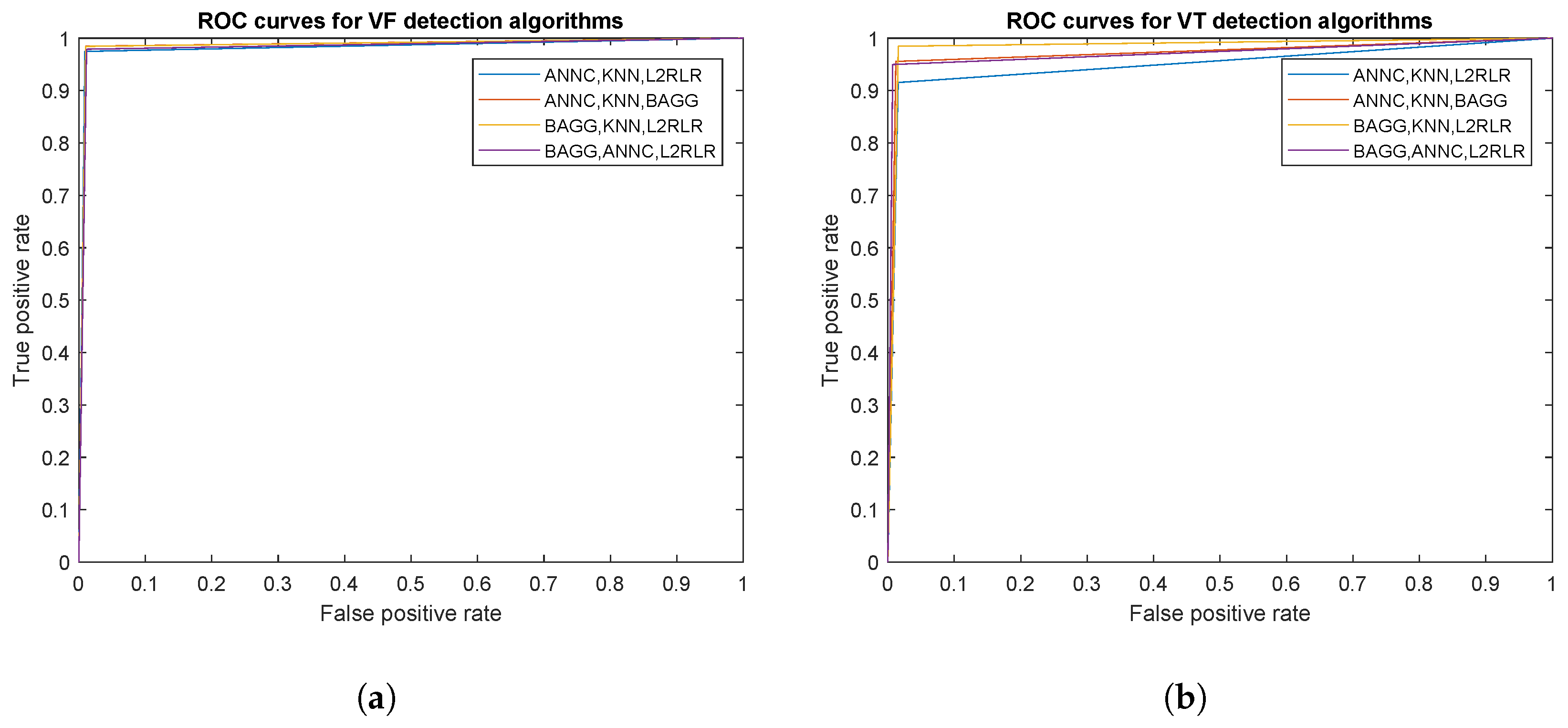
AUC(VT)	93.48	94.16	92.33	96.43

and Figure 6 show the AUC values and ROC curves, respectively, Figure 6a for $VF$ and Figure 6b for $VT$ in case of the analyzed individual algorithms.

Table 16. AUC for VMM combination methods in detection of $VF$ and $VT$.

Algorithm	$\mathit{ANNC}\_\mathit{KNN}\_\mathit{L}2\mathit{RLR}(\%)$	$\mathit{ANNC}\_\mathit{KNN}\_\mathit{BAGG}(\%)$	$\mathit{BAGG}\_\mathit{KNN}\_\mathit{L}2\mathit{RLR}(\%)$	$\mathit{ANNC}\_\mathit{ANNC}\_\mathit{L}2\mathit{RLR}(\%)$
AUC(VF)	98.28	98.72	98.70	98.36
AUC(VT)	95.03	97.18	98.44	97.12

and Figure 7 show the AUC values and ROC curves, respectively, for $VF$ (Figure 6a) and $VT$ (Figure 6b) classification results for the VMM combination of classifiers.

Table 17. AUC for HM classification combination methods in detection of $VF$ and $VT$.

Algorithm	$\mathit{ANNC}\_\mathit{KNN}\_\mathit{ANNC}(\%)$	$\mathit{ANNC}\_\mathit{KNN}\_\mathit{L}2\mathit{RLR}(\%)$	$\mathit{ANNC}\_\mathit{KNN}\_\mathit{L}2\mathit{RLR}(\%)$	$\mathit{ANNC}\_\mathit{KNN}\_\mathit{L}2\mathit{RLR}(\%)$	$\mathit{ANNC}\_\mathit{KNN}\_\mathit{L}2\mathit{RLR}(\%)$	$\mathit{BAGG}\_\mathit{KNN}\_\mathit{ANNC}(\%)$
AUC(VF)	97.11	96.98	97.44	97.44	96.13	95.77
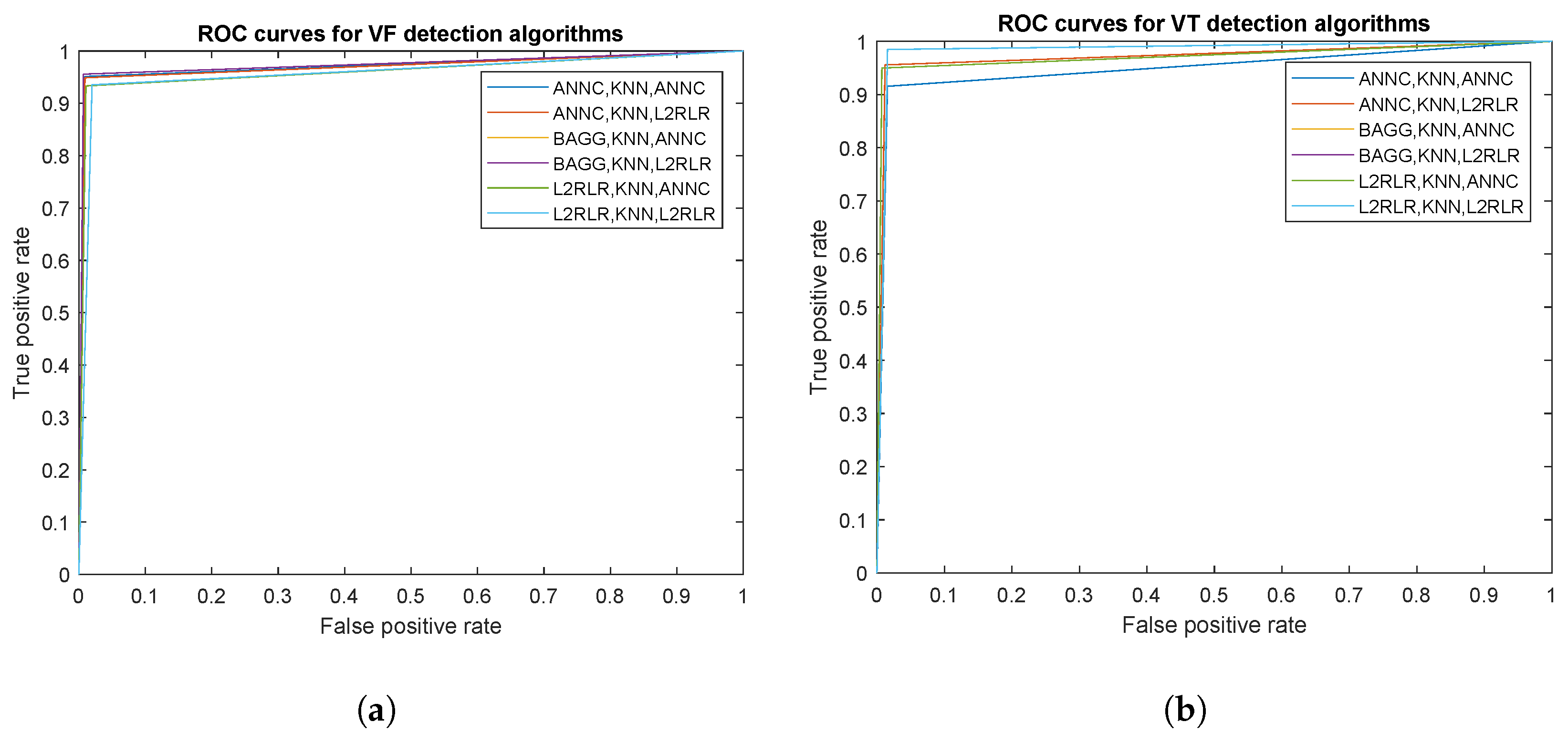
AUC(VT)	95.00	97.18	98.44	97.12	97.12	98.44

and Figure 8 show the AUC values and ROC curves, respectively, for $VF$ (Figure 6a) and $VT$ (Figure 6b) classification results for the HM combination of classifiers. As shown, ROC curves are more adjusted in case of combined classifiers, especially in case of the VMM method.

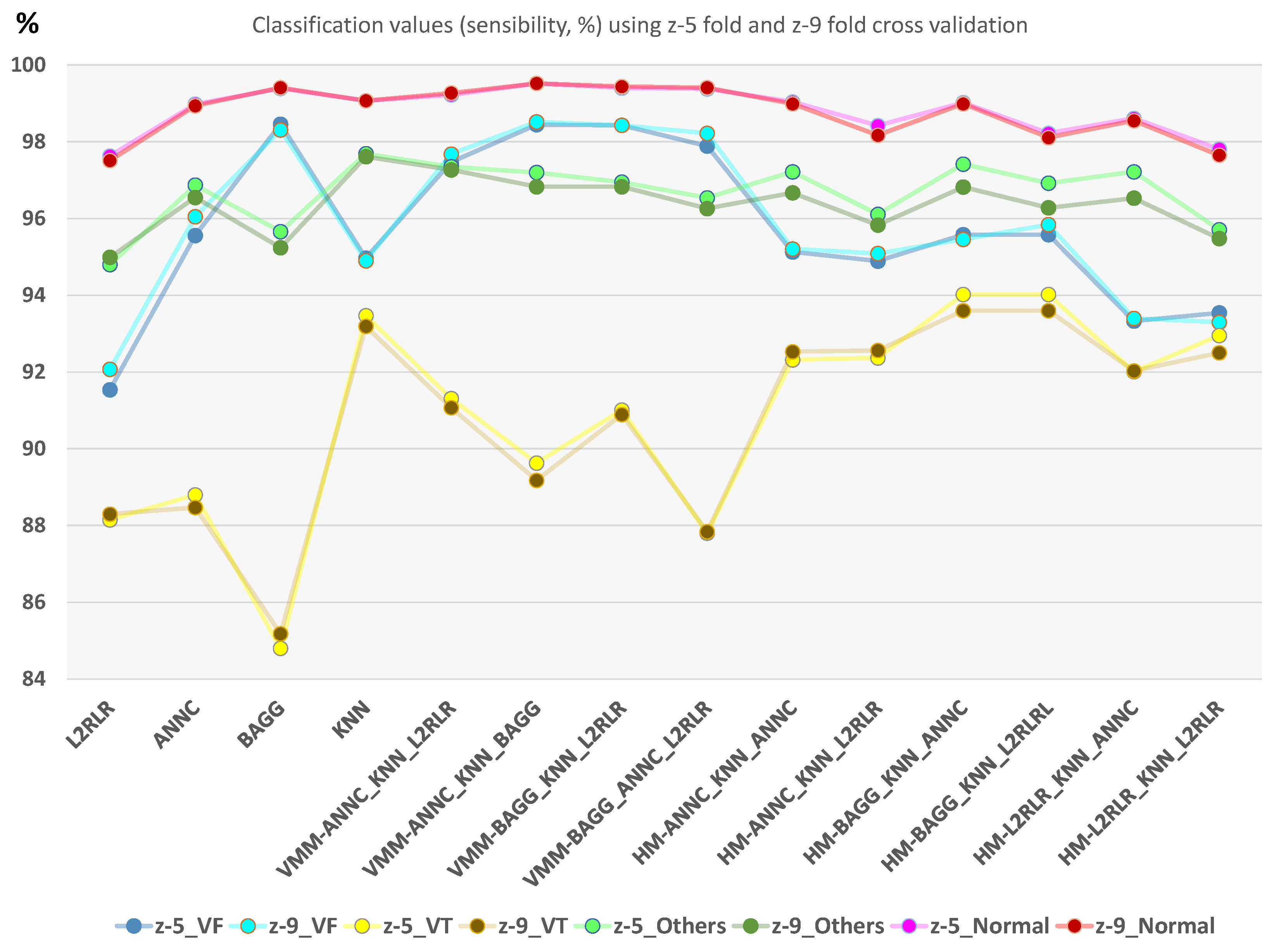
Additionally, the structural risk of the classifier is important in order to determine the training robustness. A risk test is proposed by the A-test where multiple z-fold cross-validation are performed in order to assess how classification error evolves. In this case, we have also tested 9-fold cross validation for comparison purposes with 5-fold. Figure 9 shows that very similar results are obtained for the same classifier. Specially in case of HM combined classifers, z-5 provides a slightly higher classification ratio. In any case, differences between z-5 and z-9 in the same classifier do not exceed 1% in classification value.

Since correct detection and classification of $VF$ and $VT$ is of pivotal importance for an automatic external defibrillation and patient monitoring, they should be able to distinguish $VF$ and $VT$ accurately. If $VT$ was misinterpreted as $VF$, a high-energy defibrillation would be delivered, which could damage the heart. If $VT$ is misinterpreted as $VF$, the low-energy cardioversion may not return the heart to its normal sinus rhythm, which could be fatal [34]. However, clear distinction between ventricular arrhythmia rhythms and normal or other arrhythmias is required, preventing the patient to be unnecessarily exposed to an electrical cardioversion.

As previous results show, the proposed methods obtain a high accuracy, not only in $VF$ and $VT$ separation but also in $Normal$ and $Others$. This fact leads to further separate the $Others$ class into other sub-classes where different heart pathologies could also be detected: Premature Ventricular Complex (PVC) in bigeminy or trigeminy, hypertrophy, idioventricular Rhythms, asystoles, etc. Thus, using a new classifier level, all rhythms detected as $Others$ could enter into a new classification process in order to discern among other cardiac pathologies.

Table 18. Performance evaluation of $VF$ detection algorithms for comparison with the four analyzed classifiers in this work.

Types	VF			VT			Other			Normal			Data Base
Method	Sens %	Spe %	Acc %	Sens %	Spe %	Acc %	Sens %	Spe %	Acc %	Sens %	Spe %	Acc %
This work, ANNC(t-f)	95.56	98.80	98.19	88.80	99.52	98.87	96.86	99.55	99.57	98.98	97.72	98.40	AHA & MIT-BIH
This work, BAGG(t-f)	98.46	98.43	98.44	84.58	99.86	98.82	95.66	99.87	98.95	99.39	97.61	98.57	AHA & MIT-BIH
This work,$KNN$(t-f)	94.97	99.27	98.47	93.47	99.39	98.97	97.69	99.40	99.03	99.07	98.29	98.71	AHA & MIT-BIH
This work,$BAGG\_KNN\_ANNC$(t-f)	95.58	99.31	98.6	94.02	99.31	99.14	97.42	99.52	99.07	99.02	98.36	98.72	AHA & MIT-BIH
[35], using Boltzmann	92.52			76.01			81.04						MIT-BIH
[1], using Discriminant Analysis	94.10	93.80											AHA & MIT-BIH
[36], using Filter and Counts	94.40	95.90	94.7										AHA & MIT-BIH
[37], using SVM	96.20	96.20	96.3										AHA & MIT-BIH
[38], using Lempel-Ziv and EMD	98.15	96.01	97.1										CU & MIT-BIH
[39], using Fuzzy Simil App Entropy	97.98	97.03	97.5										CU & MIT-BIH
[39], using Approximate Entropy	91.84	90.2	91.0										MIT-BIH
[40], using EMD & App Entropy	90.47	91.66	91.2										MIT-BIH
[41], using KNN	98.10	88.00	93.2										MIT-BIH
[41], using RBF	91.53	90.91	91.3										MIT-BIH
[42], using Type 2 fuzzy			90.9			84.0						100	MIT-BIH
[42], using Neural SOM			100.0			48.0						88	MIT-BIH
[43], using Type 2 TSK Fuzzy			93.3			92.0						100	MIT-BIH
[43], using Type 2 Mamdani Fuzzy			86.6			88.0						100	MIT-BIH
[44], using Random Forest Classifier	95.04	94.78	94.79										CU &MIT-BIH
[45], using SVM	95	99											CU &MIT-BIH
[46], using Binary Decision Tree (BDT)	95.3	94.5	94.2										CU &MIT-BIH
[46], using SVM	90.4	91.6	89.3										CU &MIT-BIH
[47], using LS-SVM classifier with RBF kernels	85.20	82.46	83.75										CU &MIT-BIH

compares results with different studies in the bibliography to check to what extent the obtained data support our hypothesis. Although different works are roughly comparable, we set two different groups for better comparison: those works aiming to distinguish between $VF$ and $VT$, and those works classifying multiple rhythms.

For the first group, Xie et al. [39] used approximate entropy to distinguish between $VF$ and $VT$ with performance ratios of Sens = 91.84% to $VF$, Spe = 90.2%, Acc = 91.0%, using similar signal sources than our work. In addition, they also proposed a modified version using fuzzy similarity-based approximate entropy that, in turn, got high performance ratios (Sens = 97.98% to $VF$, Spe = 97.03%, Acc = 97.5%). Although we obtained higher values, to make a fair comparison between both analysis, it has to be taken into account that Xie used representative and clean episodes of $VT$ and $VF$ as input data, in front of our work that used a multiclass scheme, classifying four types of rhythms and considering complete patient’s registers as the input signal. The same happens for other studies distinguishing between $VF$ and $VT$ rhythms; Kaur and Singh [40] used approximate entropy with Empirical Mode Decomposition (EMD) and a more reduced dataset than Xie, having good performance values (Sens = 90.47 to $VF$, Spe = 91.66%, Acc = 91.2%). Later, Xia et al. [38] also used, in the same line, Lempel-Ziv Complexity and EMD in the same conditions that Xie did before, using a representative number of clean episodes of each pathology, and they also got high performance ratios (Sens = 98.15% to $VF$, Spe = 96.01%, Acc = 97.1%). The same occurred to Li et al. [37] using SVM where Sens = 96.20% to $VF$, Spe = 96.20%, and Acc = 96.3%, for a 2 s window, was obtained; in this case, a sensitive different set of source signals was used. Other works provides good performance ratios distinguishing between $VF$ and $VT$ when applied to compressed ECG signals [41]. In all cases, our performance results are slightly or sensitive better.

As a second group of comparable works we can find those aiming to distinguish normal sinus (N) apart from $VT$ or $VF$. Within this group, Tan et al. [42] obtained good accuracy ratios (Acc($VF$) = 90.9%, Acc($VT$) = 84.0%, Acc(N) = 100%) using a type-2 fuzzy logic-based classifier for a three class multiclass classification ($VF$, $VT$ and $Normal$). Tan also described the results of using a SOM neural network with poor VT accuracy. Later, Phong et al. [43] followed the same line implementing another multiclass classifier using a type-2 TSK fuzzy system, with the same three classes than Tan used; in this case, with better accuracy ratios (Acc($VF$) = 93.3%, Acc($VT$) = 92.0%, Acc(N) = 100%). They also tried a a type-2 Mandami fuzzy system with lower values.

Other works analyse a binary distinction between $VF$ and non-$VF$ rhythms. Verma et al. [44] used 17 features: Morphological, spectral, and complexity. Here, the random forest classifier has been used for discrimination between $VF$ category and non-$VF$ category, with Acc = 94.79%, Sens = 95.04%, Spe = 94.78%. In [45], they used 13 parameters accounting for temporal (morphological), spectral, and complexity features of the ECG signal, using an SVM to distinguish between $VF$ and non-$VF$ categories with Sens = 95%, Spe = 99%. In another attempt [46], different heart rhythms were detected and classified into the $VF$ and non-$VF$ types using six features, four are derived from image-based phase plot analysis, one is derived in the frequency domain, and the last reflects the nonlinear characteristics of a data segment, values of (Acc = 95.3%, Sens = 94.5%, Spe = 94.2%) and (Acc = 90.4%, Sens = 91.6%, Spe = 89.3%) using binary decision tree (BDT) and the SVM, respectively. The algorithm proposed by Tripathy et al. [47], using digital Taylor-Fourier transform (DTFT) features of ECG signals and least square support vector machine (LS-SVM) with linear and radial basis function (RBF) kernels for detection of $VF$ and non-$VF$ arrhythmia episodes, obtained performance values of Acc = 83.75%, Sens = 85.20%, Spe = 82.46%.

Other authors have classified the ECG signal segments into $VFVT$ and non-$VFVT$. These results are not directly comparable with those in the previous table since they provide a binary output. However, we include them since they are interesting to see how simpler two-class classification still provides similar results to those obtained in this work. Zhou et al. [48] classified the ECG signal segments into the normal sinus rhytnm (NSR) or arrhythmic shockable classes $VFVT$. The classification is based on Time-Delay Transform (TDT) of the signals and a neural network with Weight Fuzzy Membership Functions (NEWFM). They obtained Acc = 89.5%, Sens = 73.6%, and Spe = 93.5%. Xu et al. [49] detected $VFVT$ using boosted classification and regression tree (Boosted-CART) obtaining Acc = 98.29%, Sens = 97.32%, and Spe = 98.95%. Other studies that have also used the class $VFVT$ [1] have evaluated both time domain (e.g., energy, permutation entropy) and frequency domain (e.g., renyi entropy) features. The classification is done by using a Random Forest (RF) classifier aiming to identify shockable and non-shockable ventricular arrhythmia with CUDB and MITDB databases with results of Acc = 97.23%, Sens = 96.54%, Spe = 97.97% [50]. Thirteen time-frequency and statistical features were extracted and applied to the C4.5 classifier [51], resulting in Acc = 97.02%, Sens = 90.97%, Spe = 97.86% for $VFVT$ detection (including ventricular flutter). In Kimmo et al. [52], gaussian processes were used to detect $VT$, $VFL$, and $VF$ episodes (all three considered in the same class) extracting 15 metrics obtaining Acc = 91%, Sens = 89%, Spe = 88%.

9. Conclusions

As mentioned above, one of the main causes of sudden death is caused by the VF arrhythmia [3,53]. The rapid and correct detection of $VF$ and $VT$ is of fundamental importance both for the use of an automatic external defibrillator and for monitoring the patient. In order to obtain a reliable algorithm to discriminate between the different arrhythmias, an attempt was made to perform this detection task using the lowest computational load. The methodology uses the ECG to monitor biomedical signals that have different morphological and spectral characteristics.

We propose the analysis of the ECG signal for the real-time detection of the onset of ventricular fibrillation using a time-frequency method [7,54]. Reduction of network interference and other noises, which correspond to high frequency noises in these signals was carried out. After performing the steps above, the data matrix of each $TFR$ is converted to an image ($TFRI$) corresponding to the different cardiac pathologies of the processed ECG signal, allowing to obtain an appropriate representation capable of providing useful information about the problem to be solved and allowing practical applications to the diagnosis in real time. The novelty of this work lies in the fact of using a reference mark $WRM$ to establish an analysis window $t_w$, obtaining a time-frequency representation and its associated image ($TFR$ and $TFRI$ matrices, respectively) which are used as input to a combined classification algorithm without calculation of additional parameters for the classifier. This fact avoids the extraction of characteristics and thus, the loss of relevant information to discriminate between the different classes. Additionaly, we propose the use of combined specialized classifiers to improve classification. An analysis of several combination methodologies, and a comparative study between the individual performance of the $KNN$, $ANNC$, $L2RLR$, and $BAGG$ algorithms was done. All of these individual and combined classifier algorithms were trained with the cross-validation method and evaluated based on sensitivity, specificity, accuracy, precision, and execution time.

Using the $TFRI$ strategy, we concluded that, using z-5 cross validation, the individual $KNN$ classifier achieves good results retrieving a sensitivity of 94.97 ± 0.70%, a specificity of 99.27 ± 0.05%, an accuracy of 98.47 ± 0.01%, and a precision of 97.09 ± 0.14% for $VF$. In case of $VT$, a sensitivity of 93.47 ± 0.19%, specificity of 99.39 ± 0.15%, accuracy of 98.97 ± 0.08%, and precision of 92.11 ± 0.7%, with a running time $t=0.17$ s. Using the $TFRI$ strategy with combined classifiers in hierarchical form (HM) achieved a sensitivity of 95.58 ± 0.40%, specificity of 99.31 ± 0.08%, 98.6 ± 0.04% accuracy, and a precision of 98.25 ± 0.29% for $VF$, with a sensitivity of 94.02 ± 0.58%, specificity of 99.31 ± 0.08%, accuracy of 99.14 ± 0.43%, and a precision of 98.59 ± 0.09% for $VT$, with execution time between $0.07$ s and $0.12$ s.

Different classifier robustness and classification analysis are performed to validate results: Sensibility, specificty, accuracy, precision, confusioin matrices, ROC, AUC, and A-test. All these analyses show that the used methodology is adequate and congruent results are obtained.

Taking into consideration the performed study, we have concluded that the use of combined classifiers is the best way to integrate the information since they provide stronger and efficient estimates than a single classifier. The proposed methodology provides useful information for the detection of $VF$ in real time with a low computational time, discriminating $VF$ from the rest of the cardiac pathologies satisfactorily. This fact significantly improves the possibilities of correct diagnosis of the patient when presenting an episode with any of these arrhythmias.