Thin Cap Fibroatheroma Detection in Virtual Histology Images Using Geometric and Texture Features

Abstract

Atherosclerotic plaque rupture is the most common mechanism responsible for a majority of sudden coronary deaths. The precursor lesion of plaque rupture is thought to be a thin cap fibroatheroma (TCFA), or “vulnerable plaque”. Virtual Histology-Intravascular Ultrasound (VH-IVUS) images are clinically available for visualising colour-coded coronary artery tissue. However, it has limitations in terms of providing clinically relevant information for identifying vulnerable plaque. The aim of this research is to improve the identification of TCFA using VH-IVUS images. To more accurately segment VH-IVUS images, a semi-supervised model is developed by means of hybrid K-means with Particle Swarm Optimisation (PSO) and a minimum Euclidean distance algorithm (KMPSO-mED). Another novelty of the proposed method is fusion of different geometric and informative texture features to capture the varying heterogeneity of plaque components and compute a discriminative index for TCFA plaque, while the existing research on TCFA detection has only focused on the geometric features. Three commonly used statistical texture features are extracted from VH-IVUS images: Local Binary Patterns (LBP), Grey Level Co-occurrence Matrix (GLCM), and Modified Run Length (MRL). Geometric and texture features are concatenated in order to generate complex descriptors. Finally, Back Propagation Neural Network (BPNN), kNN (K-Nearest Neighbour), and Support Vector Machine (SVM) classifiers are applied to select the best classifier for classifying plaque into TCFA and Non-TCFA. The present study proposes a fast and accurate computer-aided method for plaque type classification. The proposed method is applied to 588 VH-IVUS images obtained from 10 patients. The results prove the superiority of the proposed method, with accuracy rates of 98.61% for TCFA plaque.

1. Introduction

Heart disease is the most common cause of death worldwide. The usage of an automatic image processing method to diagnose heart disease is one of the most significant medical research areas [1]. The cause of most acute coronary syndromes (ACS) is often the rupturing of vulnerable plaques [2]. Although thin cap fibroatheroma (TCFA) lesions cause the most myocardial infarctions, reliable identification of TCFA remains a demanding challenge [3]. Plaque phenotype and composition appear to be related to plaque instability. Therefore, distinguishing between plaque types is necessary to detect vulnerable plaque [4]. The Virtual Histology-Intravascular Ultrasound (VH-IVUS) is an invasive imaging technique to analyse the internal morphology of coronary arteries. VH-IVUS has been proposed based on the 20 MHz IVUS platform for studying in-vivo plaque compositions [5]. Recent studies have shown that VH-IVUS can identify the high-risk plaques [6]. Apparently, development of quantitative techniques represents a practical approach to predict and quantify plaque compositions [7]. However, there are no proper automatic tools for feature extraction using VH-IVUS [8]. Nair et al. [9] introduced the first commercially available IVUS, based on Volcano (Volcano Corporation, San Diego, CA, USA) IVUS clinical scanners [10]. Volcano’s technology classifies four tissue types of plaque by means of spectral analysis methods with an accuracy of 93–97% [11]. However, the number of characterised IVUS frames is limited due to the Electrocardiogram (ECG)-gated acquisition. In fact, at each cardiac cycle, only one VH-IVUS image is characterised by RF spectrum. VH-IVUS images are generated at a rate of one frame per second; whereas, the rate of producing IVUS images is 30 frames per second [12]. It is worth noting that this commercial package has certain limitations in terms of extracting the significant features for TCFA detection. For instance, if the necrotic core (NC) is scattered, VIAS (Volcano Corporation, San Diego, CA, USA) can identify a single area measurement, but only the confluent NC in contact with the lumen is important [13]. Moreover, lumen border detection by employing VIAS software may provide unreliable results due to the border degradation caused by jpg image compression [13].

Extracting a useful feature set for classification is a challenging issue. Various techniques of feature analysis, such as brightness, contrast, colour, or texture, can be described comprehensively based on an image’s appearance [14]. Geometrical features are often local in nature, so spatial information will not be considered [15]. For this purpose, texture features are defined for analysis of micro textures [16]. Texture can be considered to be a global pattern involving the repetition of local sub patterns [17]. This approach analyses spatial variations of pixel intensities and quantifies them into numerical values. Texture-based methods are very useful in providing descriptors for homogeneous regions [18]. VH-IVUS images comprise various granular patterns at different scales called “texture”, related to the smoothness, roughness, and regularity of any patterns [19]. Based on previous studies, texture analysis is useful to measure the plaque compositions in ultrasound images. Due to the varying texture patterns of plaque components, texture descriptors have been applied for analysis of plaque compositions [20]. When considering statistical texture-based methods, Grey Level Co-occurrence Matrix (GLCM) and Grey Level Run Length Matrix (GLRLM) descriptors remain among the top choices [21]. Based on the proposed criteria in [21], a subset of GLCM and Run Length (RL) descriptors maximises the classification accuracy of the training dataset. Furthermore, the efficacy of GLCM, Local Binary Patterns (LBP), Gabor filters, and RL method is demonstrated for plaque assessment [22]. To describe the local information of a pattern, LBP algorithms can be adopted, while the overall texture information can be described by GLCM algorithm [23]. It is often necessary to characterise the tissue appearance of medical images by smoothness, grain, regularity, and homogeneity by applying various texture descriptors; Run-length method describes the coarseness of a texture in the specified linear orientation [19].

Escalera, Pujol, Mauri and Radeva [7] described IVUS tissues by means of different types of features: radial frequency, texture-based features, and combined features. Three different texture descriptors were applied, including co-occurrence Matrix, LBP, and Gabor filters. Athanasiou et al. [24] proposed a semi-automated method for plaque characterisation. To classify the tissue type, textural features, comprising co-occurrence matrices, LBPs, mean value, entropy, intensity, and geometrical features, were extracted for each pixel. Giannoglou et al. [25] applied a set of different textural features consisting of first order (FO) statistics, GLCM, WF, RL, and LBP for tissue labeling. Katouzian et al. [26] presented a texture-based method by applying discrete wavelet packet frame (DWPF) for labelling the atherosclerotic plaque. Taki, Roodaki, Setarehdan, Avansari, Unal and Navab [20] proposed an image-based method for characterisation of coronary plaques in IVUS images. A combination of grey-scale-based features and textural descriptors, including LBP, MRL, and Neighbouring Grey-Level (NGL) are extracted to categorise each pixel into one of the three classes (DC, NC, and FF). A fully automated method is presented by Dehnavi et al. [27] to classify the soft and hard plaque. After border detection, FCM method classified the GLCM features. Giannoglou and Theocharis [22] extracted a set of textural features, including first order (FO) statistics, wavelet features (WF), GLCM, RL, and LBP with different scales to improve the plaque type classification. Therefore, in this study, three commonly used textural features, including LBP, GLCM, and MRL, are extracted from VH-IVUS images.

Due to the increased noise, artefacts, and mixed tissue in VH-IVUS images, the studied methodologies may not be suitable for providing accurate results of segmentation. Furthermore, most of the presented approaches are semi-automated. Some approaches are time consuming and involve expert corrections to refine the results. Developing a robust image segmentation approach may be a complicated problem [28]. The aim of this research is to improve the identification of TCFA in VH-IVUS images by improving VH-IVUS image segmentation and vulnerability detection. Therefore, hybrid Fuzzy C-means with Particle Swarm Optimisation (PSO) and minimum Euclidean distance algorithm (FCMPSO-mED) and Hybrid K-means with PSO and minimum Euclidean distance (KMPSO-mED) models are adapted based on the semi-supervised learning theory. FCMPSO-mED and KMPSO-mED can classify the unlabelled data without requiring the training data. Therefore, it improves the accuracy of pixel classification when sufficient training data are not available. The rest of this paper is structured as follows. Section 2 describes the related works. The proposed approach for segmentation, feature extraction, and TCFA detection are described in Section 3. Validation and comparison with existing methods are described in Section 4. The proposed methodology is discussed in Section 5. Finally, the paper is concluded in Section 6.

2. Related Works

IVUS image segmentation is often an essential step for characterisation of vessels, comprising shape, area, eccentricity, and thickness [8]. Generally, segmentation is an essential process for identifying image structures that can be completed using a manual, semi-automatic, or automatic method [29]. IVUS images consist of three basic parts: intima, media, and adventitia. The intima layer refers to the vessel interior. However, the adventitia represents the vessel outer layer, also characterised by flexible tissue. The media part discriminates the intima from the adventitia [30].

The segmentation of atherosclerotic plaques has been addressed in several studies. Dhawale et al. [31] proposed the first semi-automated technique for IVUS border detection by dynamic search algorithm. Similarity, a primary work was presented by Sonka et al. [32] for detection of media and lumen borders by applying heuristic graph searching and global image information. A fully automated segmentation step and a user-guided refinement stage for segmentation of luminal and external elastic lamina surface was presented by Sun et al. [33]. Jones et al. [34] presented a user-assisted method for media–adventitia border segmentation in IVUS images. To detect the media–adventitia border, fully automatic approaches were presented in [35,36]. Automatic techniques to detect the lumen border are also presented in [37,38,39,40]. However, some studies have proposed fully automated segmentation methodologies for plaque border detection [8,41,42,43]. Automatic approaches for lumen and media adventitia border detection and plaque characterisation have been adapted, as well [44]. A comparison of the above-described IVUS image segmentation methods is presented in

Table 1. IVUS image segmentation overview.

Source	Segmentation	Technique	Advantages	Disadvantages
Dhawale, Rasheed, Griffin, Wilson and Hodgson [31]	Dynamic search algorithm	Semi-automatic	Proposed the first IVUS image segmentation method. The outer media–adventitia border can be detected with only one user point.	Time consuming Requiring expert’s annotations for each frame.
Sonka, Zhang, Siebes, Bissing, DeJong, Collins and McKay [32]	Heuristic graph searching and global image information	Semi-automatic	Identification of optimal border. Excellent agreement of the computer-detected and observer-defined lumen areas.	Needs to user interaction. Needs to resample data to form a straightened image. Examines only in vitro images.
Plissiti, Fotiadis, Michalis and Bozios [41]	Deformable model	Automatic	It reduced the noise in IVUS images. Result was close to those provided by experts. Fast computation. Method is automatic even for calcified regions.	Borders Detection in the first IVUS frame was done manually. Requires to be improved for solving the issue of side branches.
Giannoglou, Chatzizisis, Koutkias, Kompatsiaris, Papadogiorgaki, Mezaris, Parissi, Diamantopoulos, Strintzis and Maglaveras [42]	Deformable model	Automatic	It reduced the noise in IVUS images. Result was close to those provided by experts. Fast computation. Automatic detection of calcified regions.	Borders Detection in the first IVUS frame was done manually. Requires to be improved for solving the issue of side branches.
Taki, Najafi, Roodaki, Setarehdan, Zoroofi, Konig and Navab [43]	Active contours and level sets	Automatic	High speed of feature extraction by applying Bayes classifier. Shadow detection. Characterisation of calcified region.	Fibrous and lipid components are not characterised.
Katouzian, Angelini, Angelini, Sturm, Andrew and Laine [37]	Brushlet Analysis and Fourier Domain	Automatic	Delineates lumen borders of high-frequency image. Isolates coherent area from incoherent ones.	Low data sample.
Zhu, Zhang, Shao, Cheng, Zhang and Bai [8]	Gradient vector flow snake model	Automatic	Applies nonlinear filtering to reduce the critical points. Automatically initialises and overcomes the problem of local energy minima.	It may fail for segmentation of poor-quality images.
Essa, Xie, Sazonov and Nithiarasu [36]	Graph cut	Automatic	Combines local and global features. Prevents undesirable image features from interfering the segmentation task.	Low data sample
Ciompi, Pujol, Gatta, Alberti, Balocco, Carrillo, Mauri-Ferre and Radeva [35]	Holistic approach	Automatic	Many frames can be quickly analysed without any manual intervention. Holistic method is potentially applicable to any image.	IVUS data is labelled manually.
Athanasiou, Karvelis, Sakellarios, Exarchos, Siogkas, Tsakanikas, Naka, Bourantas, Papafaklis and Koutsouri [44]	deformable models	Automatic	Combined Feature (intensity, texture and, geometrical). Multi classifier.	Area behind a calcific deposit was not detected. Performance relies on consistency of observers.
Sun, Sonka and Beichel [33]	Graph-based	Automatic segmentationanduser-guided refinement	Produces high-quality segmentation results in cases of artefacts. Reduces time of segmentations. Close-to-real-time IVUS segmentation.	Fails segmentation in zigzag pattern. Needs to adjust the surface smoothness between adjacent IVUS images. The vessel is assumed to be without bifurcations.
Lazrag, Aloui and Naceur [38]	FCM algorithm and active contours	Automatic	Approximates efficiently the boundary by FCM. Refines the final lumen by level set method.	High-level knowledge is needed to control the motion of level set contours.
Mendizabal-Ruiz, Rivera and Kakadiaris [39]	Deformable curve	Automatic	Segmentation of B-mode images from different systems and transducer frequencies. Robustness with the changes of B-mode parameters.	Samples of blood and non-blood areas in the first frame are needed. Dependence on annotations for the first frame. Inaccurate IVUS images segmentation with artefacts.
Jones, Essa, Xie and Smith [34]	Graph-cut	User-assisted	Adopted layered graph representation to simplify computation. Efficient interactive segmentation images with artefacts.	Initial seed points of Graph cut are set manually.
Sofian, Ming and Noor [40]	Otsu threshold	Automatic	Achieves reasonably good segmentation results compared to the manual tracings. Consistent for all IVUS samples.	Further improvement is needed to get better result. Low performance for measuring Hausdorff Distance.

.

Although there are several existing works in the literature in the domain of TCFA detection, it still remains a challenging task [3]. In our previous work [45], hybrid Fuzzy C-means and K-Nearest Neighbour (HFCM-kNN) was proposed to accurately segment VH-IVUS images. The proposed technique was capable of eliminating outliers and detecting clusters with different densities in VH-IVUS images. The next process was extracting the geometric features to provide an accurate definition of the vulnerable plaque. Machine learning approaches were applied for training the in-vivo images obtained from different patients. The major contribution of this paper is to improve VH-IVUS image segmentation using a semi-supervised approach. The K-means and PSO (KMPSO) model is hybridised with the mED algorithm to more accurately segment the VH-IVUS image. Typically, texture features have proven to be useful in describing the medical images [46]. Due to the heterogeneity of the atherosclerotic tissues, a robust texture discriminator needs to be developed [26]. However, in our previous work [45], only geometric features were extracted and fed to the classifiers. Therefore, the second contribution of this work is with regard to hybrid geometric and texture features, whereas existing research on TCFA detection has only focused on geometric features. Moreover, classification is performed by machine learning algorithm to optimally discriminate TCFA and non-TCFA plaque. As VH-IVUS is commercially available, the methodology proposed in this study can be implemented with other methods, such as iMap (Boston Scientific, Marlborough, MA, USA) and IVUS image-based techniques.

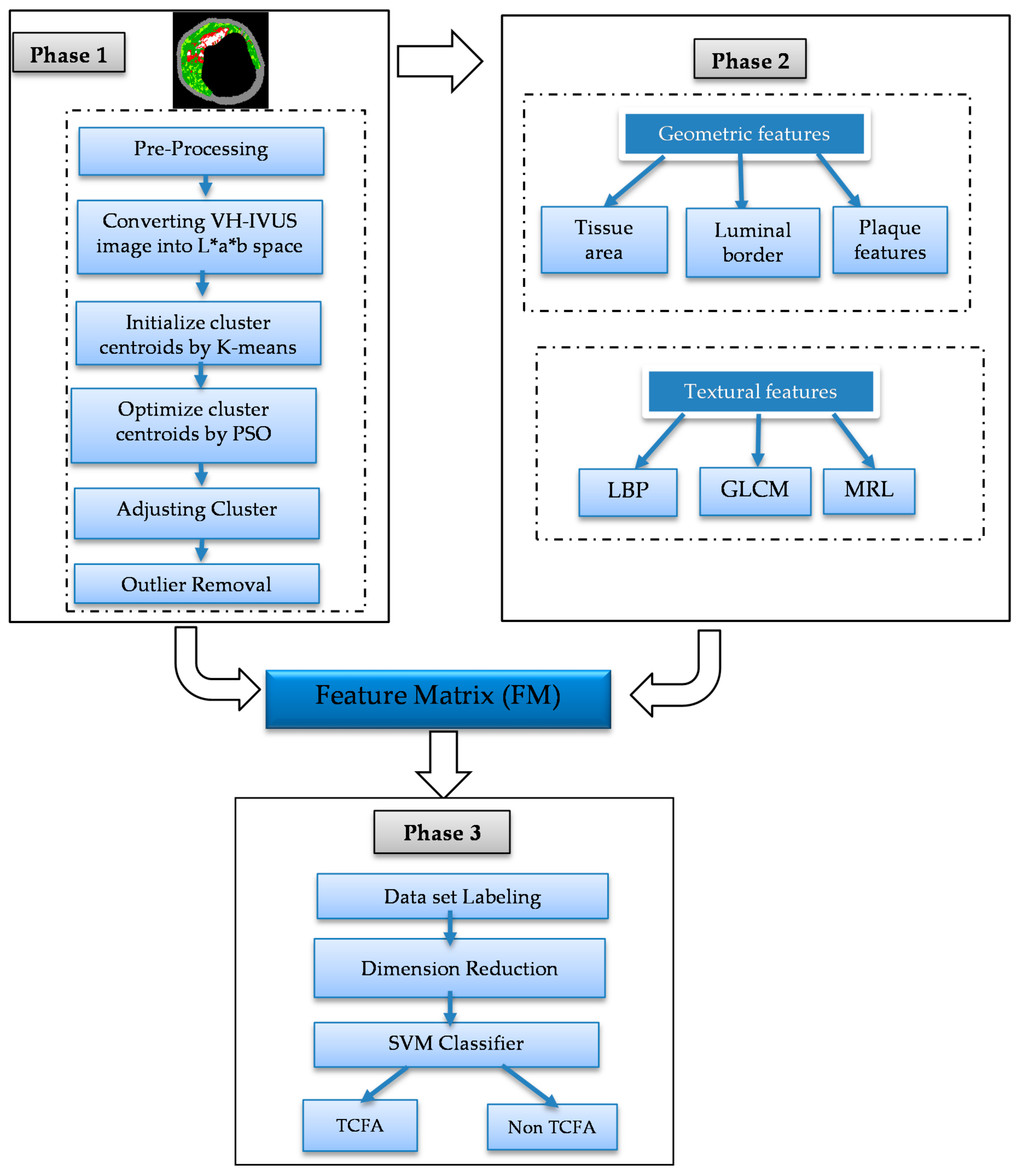
3. Proposed Approach

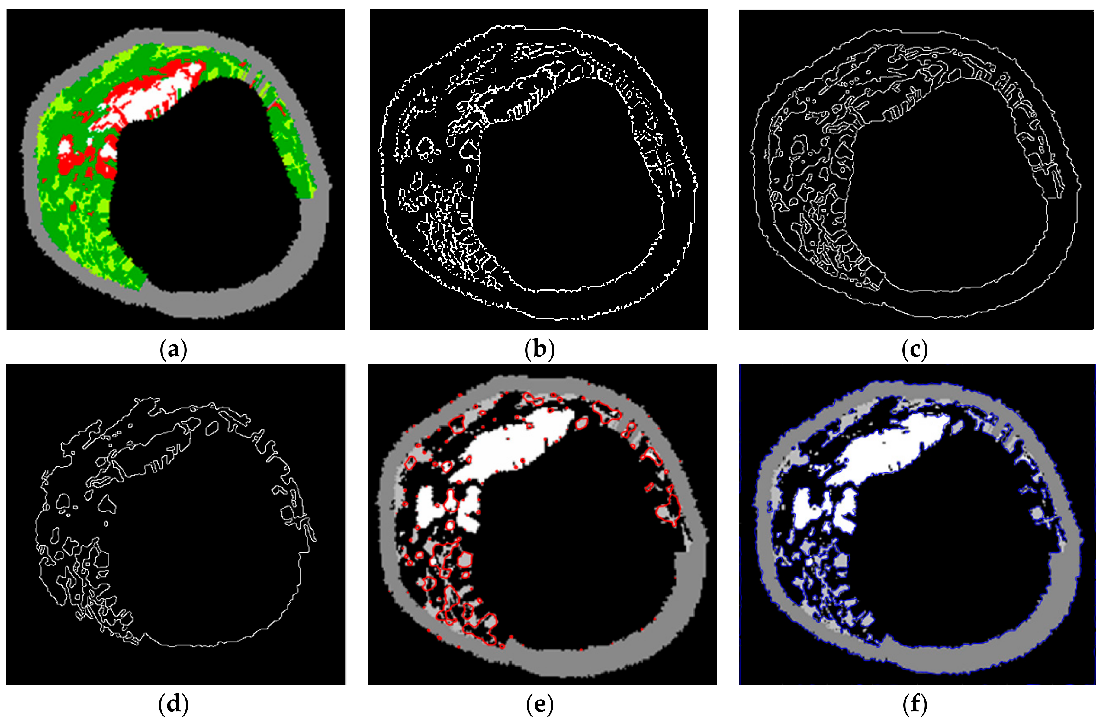
The proposed approach consists of three main phases. Phase 1 shows the steps for VH-IVUS image segmentation using a semi-supervised model, namely, KMPSO-mED. The KMPSO-mED algorithm first executes the K-means algorithm to seed the initial swarm. The PSO algorithm is then applied to optimise the seed points. After the clustering process, cluster labelling is applied, and the colour feature matrix is extracted from the segmented images [45]. Pixel-wise classification is performed to test the image using the proposed algorithm, namely, mED. In Phase 2, geometric features, including luminal border, plaque component and texture features, are extracted from the VH-IVUS image. Finally, in Phase 3, Back propagation (BPNN), kNN (K-Nearest Neighbour), and Support Vector Machine (SVM) classifiers are applied to select the best one for classifying the plaque into TCFA and Non-TCFA. The best classifier is selected to classify the geometric and texture features. A block diagram of the proposed approach is presented in Figure 1.

A graphic user interface (GUI) can be designed as an effective VH-IVUS image processing tool, enabling cardiologists to complete lumen border detection, segmentation, plaque characterisation, and TCFA detection. The methods proposed in this study were implemented in MATLAB R2014b software (The Mathworks, Inc., Natick, MA, USA); however, to obtain a standalone executable application, the GUI should be compiled by a C# compiler in Microsoft Visual Studio.net [47].

3.1. Segmentation

Segmentation techniques attempt to partition the different tissues into non-overlapping regions [48]. VH-IVUS image segmentation poses a challenge, since in this type of image, there is no sharp boundary between colours, including red, white, dark green, and light green [49]. As a result, reliable discrimination of these components can be more difficult [24]. Spectral overlapping of NC with DC makes the segmentation process difficult [22]. Accurate segmentation of DC and NC are also required, since when DC is next to the NC in IVUS images, DC is often coded as NC [50]. The existing technology for VH-IVUS image segmentation is based on simple thresholding approaches. This method is not always reliable for segmenting the highly mixed tissue types involved in VH-IVUS images. Developing a more accurate approach is required for classifying necrotic core, fibrotic, fibro fatty, and calcified tissues [51].

Generally, medical image segmentation can be classified into six main categories, consisting of thresholding, edge detection, region growing, shape constrained deformable model, active counter model, and clustering [29,52]. These techniques have their own advantages and drawbacks. Hence, the ability of the segmentation scheme to characterise the overlapped tissue in VH-IVUS images is explored here.

Thresholding is a common method to separate the foreground and background regions using the pixel intensity [52]. However, this technique does not guarantee the separation of regions with similar intensities, but belonging to different regions [52]. The thresholding method only uses the distribution of pixel intensity, neglecting the neighbourhood information [53]. In terms of overlap borders, determining the appropriate threshold for VH-IVUS image segmentation is rather difficult [54]. The edge detection method is generally used to detect the points with abrupt changes in the grey levels. However, this method has limitations in terms of detecting weak edges [55]. Moreover, a closed curve cannot be easily identified [52].

Region growing algorithms are able to correctly classify the regions with similar properties and performs well in segmentation of noisy images [56]. However, the conventional region growing approach has major drawbacks in terms of selecting the seed point and determining the order of regions [55]. Therefore, in order to provide satisfactory segmentation results, the initialisation should be very close to the object contour [57]. The active shape model is fast and robust for identifying object shapes. This model is robust in the presence of noise, as well as image artefacts such as missing or damaged parts. However, it can only consider the deformations in the training set and has limitations with regard to unpredicted shapes [58]. Furthermore, in order to move the contour towards the optimal boundaries, the contour should be initialised close enough to the object [54,57].

Clustering algorithms classify image pixels into k groups, whereas pixels belonging to a cluster are homogeneous [59]. The clustering methodology is considered to be very efficient at dealing with image segmentation due to the less complex mathematical models and there being no need for training data [60]. Clustering approaches have been adapted for VH-IVUS image segmentation for the following reasons:

Segmentation of poor boundaries. Clustering approaches can usually be categorised into hard and fuzzy clustering. In image segmentation, when the cluster boundaries are poorly defined, the fuzzy clustering method can be used [61].

Segmentation of overlapped borders. Based on the fuzzy concepts, the intensity value has a membership degree associated with each cluster centre. In fuzzy clustering, each data element can belong to more than one cluster with a certain membership level, whereas in hard clustering, the data belongs to only one cluster. Clustering approaches can be successfully applied to discriminate between the different tissues. However, most medical images often involve overlapping intensities at tissue borders, so pixels may belong to more than one cluster [29,62]. As a result, tissues are not always clearly distinct, and the membership values of the borders are essentially fuzzy.

Colour image segmentation. Since colour components provide more information than the grey-scale components, the clustering technique may further improve the segmentation results [55].

Dealing with unlabelled data. Clustering models can find the structure of unlabelled data [63]. These techniques measure the similarity between the unlabelled data to form clusters in an unsupervised manner [64]. These approaches consider the spatial information of the image and classify the image into different regions by means of the homogeneity criterion [52].

Unsupervised learning. In supervised algorithms, data can be labelled by applying the training set [64]. Clustering approaches employ the spatial information of images without the use of training data or learning stages [63]. These techniques have lower computational complexity in comparison to the supervised methods [54].

Figure 2 illustrates the result of thresholding, edge detection, region growing [65], level set [66], and active contour (sank), and Figure 3 illustrates the results of clustering using the K-means algorithm.

As illustrated in Figure 2 and Figure 3, unsatisfactory segmentation results are obtained in terms of the overlap borders in the VH-IVUS image, so an accurate algorithm should be developed.

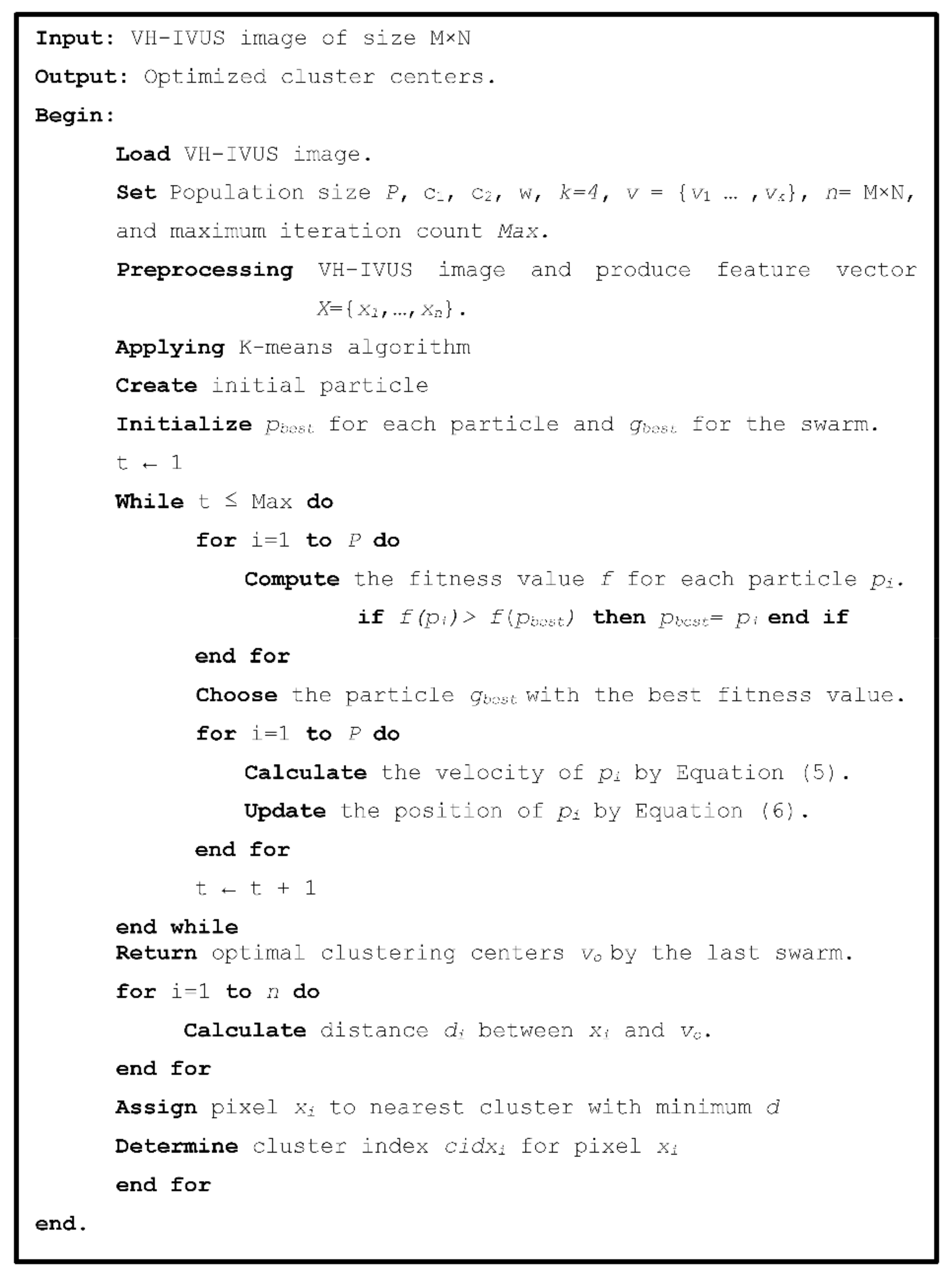
3.1.1. Proposed KMPSO-mED Model and Its Adaptation to VH-IVUS Image Segmentation

K-means and FCM clustering mainly have drawback with respect to the pre-defined number of clusters k. However, some of the tissue may be absent in VH-IVUS images. Moreover, when the VH-IVUS images have a low-density colour, clustering algorithms may combine two clusters into one cluster. An individual system faced some problems, so a combined intelligent system was applied to address the weaknesses of individual systems [67]. PSO achieves the global optimum and can be a very powerful approach for dealing with image segmentation [68]. In this section, in order to enhance VH-IVUS image segmentation, K-means and FCM clustering algorithms are hybridised with the PSO algorithm. The details of the proposed semi-supervised model are presented here.

3.1.2. Pre-Processing

A VH-IVUS image represents a matrix with dimensions M × N × 3, which are quantised as integers with a value of 0 to 255 for each fundamental colour (Red, Green, Blue) [69]. The Media–Adventitia (M–A) border, grey in colour, creates an unwanted cluster, so it can be removed from the VH-IVUS image [45].

3.1.3. K-Means Algorithm

In the first iteration, k cluster centres v = {v₁,…v_k are initialised randomly [70]. The distance between all data points X = {x₁, x₂,…x_n} and each cluster centre v_j are calculated according to the following equation:

$$d_{ji}^{\left(t-1\right)}\left(x_i,v_j\right)=\Vert x_i-v_j^{\left(t-1\right)}\Vert , i=1,2\dots n,j=1,2\dots k$$

(1)

where x_i represents the ith data point, v_j shows the jth cluster centre, and n is the number of data points. Then each sample is assigned to the nearest cluster. Class means, or cluster centres, can be updated by the following equation:

$$v_j^{\left(t\right)}=\frac{{{\displaystyle \sum }}_{x\in j}{x}_i}{n_j}$$

(2)

where n_j is the number of data points belonging to the jth cluster at the iteration t. K-means converges when the cluster centres do not change anymore based on the following equation:

$$v_j^{\left(t+1\right)}=v_j^{\left(t\right)} \forall j=1,2\dots k$$

(3)

3.1.4. Particle Swarm Optimisation (PSO)

PSO has three major steps, including generating the particles’ positions and velocities, velocity update, and position update. This algorithm has five important parameters, as presented in

Table 2. PSO parameters.

Parameters	Description
Particle	Candidate solution to a problem
Velocity	Rate of position change
Fitness	The best solution achieved
pbest	Best value obtained in previous particle
gbest	Best value obtained so far by any particle in the population

.

The random velocities and positions of all particles are initialised within the specific ranges. The values of ${\overrightarrow{p}}_{i,best}$ and ${\overrightarrow{g}}_{i,best}$ can be updated based on the fitness function f when the following conditions are satisfied:

$${\overrightarrow{p}}_{i,best}={\overrightarrow{p}}_i if f\left({\overrightarrow{p}}_{i }\right)>f\left({\overrightarrow{p}}_{i,best}\right){\overrightarrow{g}}_{i,best}={\overrightarrow{g}}_{i}if f\left({\overrightarrow{g}}_{i }\right)>f\left({\overrightarrow{g}}_{i,best}\right)$$

(4)

The fitness of a particle is calculated as the quantisation error [71]:

$$f=\frac{{{\displaystyle \sum }}_{j=1}^k[{{\displaystyle \sum }}_{\forall p_{ \in }{C}_{ij}}d\left(p,v_j\right)/\left|C_{ij}\right|]}{k}$$

(5)

where d is defined as the distance between a particle p and a centroid v_j, |C_ij| represents the number of particles belonging to the cluster C_ij, and k is the number of clusters. During the iteration, velocities of all particles are updated by:

$${\overrightarrow{v}}_i=w{\overrightarrow{v}}_i+c_1{R}_1\left({\overrightarrow{p}}_{i,best}-{\overrightarrow{p}}_i\right)+c_2{R}_2\left({\overrightarrow{g}}_{i,best}-{\overrightarrow{p}}_i\right)$$

(6)

where ${\overrightarrow{v}}_i$, ${\overrightarrow{p}}_i$, ${\overrightarrow{p}}_{i,best}$ are the velocity, position, and the local best position of particle i, respectively. ${\overrightarrow{g}}_{i,best}$ shows the global best position for the whole population. The w is used to control the convergence behaviour of the PSO algorithm, R₁ and R₂ are random variables between [0, 1], and c₁ and c₂ are used to control particle movement during each iteration. The particles’ positions can be updated by the following equation:

$${\overrightarrow{p}}_i={\overrightarrow{p}}_i+{\overrightarrow{v}}_i$$

(7)

3.1.5. Hybrid K-Means and PSO (KMPSO) Model

The combination of the K-means and PSO (KMPSO) models executes the K-means algorithm to seed the initial swarm until a termination condition is reached, and the input vectors are grouped into four clusters [71]. The cluster centroids produced by the K-means algorithm are then used as one of the particles of a swarm, and the rest of the particles are initialised randomly. The PSO algorithm is then utilised to optimise the cluster centroids. This algorithm repeats for a defined number of iterations. The optimal clustering centres v_o can be obtained by the last swarm. To assign the class label, the distances between all pixels x and v_o are calculated. Figure 4 illustrates the details of the training phase of the KMPSO model.

Since clustering algorithms will not return the same cluster index value every time, the colour of each cluster should be determined. With respect to the colour of each cluster, its matching plaque components can be determined as NC: red, DC: white, FI: dark green, and FF: light green [45].

The result of the clustering algorithms will be strongly affected by the presence of outliers that do not belong to any of the clusters [28]. The purpose of outlier detection is to find small groups of pixels that are not similar to the rest of the pixels belonging to the same cluster [72]. Figure 5 illustrates the outliers with dark green, light green, etc., in an NC image. The zoomed area (b) is indicated by the blue box in the original image (a).

To provide more reliable results, outliers should be removed from the generated clusters. NC and DC images play an important role in TCFA detection; therefore, their outliers are removed for modifying the training set. First, the Euclidian distance between pixels belonging to the NC and its centre are calculated. Then, for each pixel in the NC image, if its distance is greater than the defined threshold value (T_NC), then this pixel is an outlier, and its intensity should be replaced with zero. Based on the sub experiments, the value of T_NC is changed, and intra-cluster distance (the distance between pixels and the centroid within a cluster) for the NC image are calculated. The value of T_NC = 200 gave the best result for the minimum distance between pixels of the NC and its centre. In addition, outliers of DC image are removed in the similar way [45].

Class label of each colour feature should be determined to perform the pixel wise classification [73]. The non-zero pixels in DC, NC, FF, and FI images were saved into CF matrix. Their corresponding labels were calculated and saved into the vector L [45].

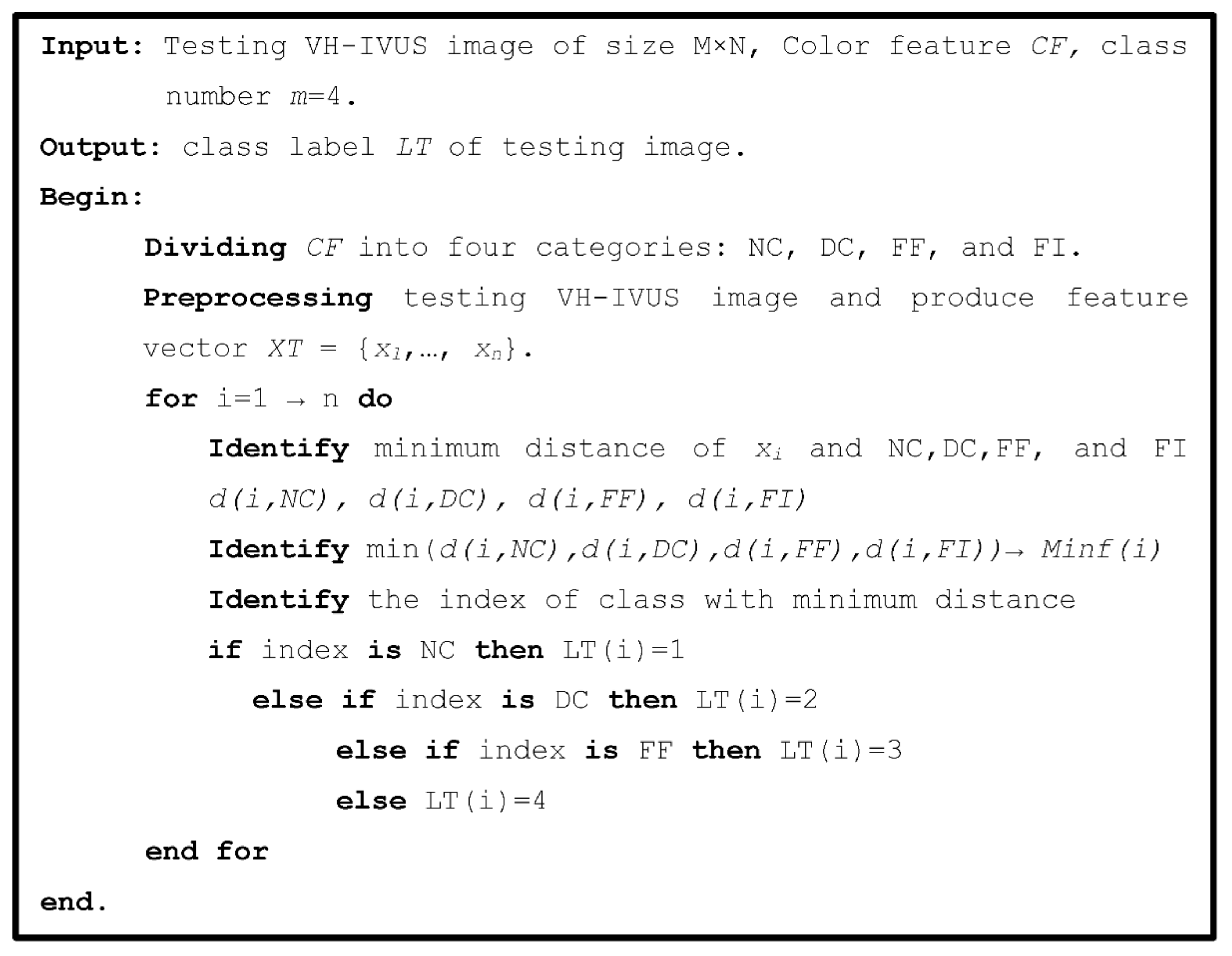
3.1.6. Pixel-Wise Classification Using Minimum the Euclidian Distance (mED) Algorithm

To address the image segmentation problem, several unsupervised and supervised approaches have been described. The supervised learning requires appropriate labelled data as training set to build a predictive model [29]. In contrast, unsupervised techniques can be explored without knowing any prior information [74].

In our previous work, k-NN algorithm was applied for pixel wise classification [45]. Although k-NN algorithm can be used for large number of training sets, but the classification is slow and time-consuming. The choice of k also affects the performance of this algorithm. Also, the accuracy of this algorithm may be degraded in presence of noisy or irrelevant features [56]. Therefore, a new algorithm namely Minimum Euclidian distance (mED) is proposed to classify the pixels in testing images. This algorithm does not require any training data and uses the colour feature matrix CF. For pixel classification by mED algorithm, feature matrix CF is divided into four classes: NC, DC, FF, and FI. The minimum Euclidian distance between testing sample x_i and those classes are then calculated and represented as MinClass_i = {min_NC, min_DC, min_FF, min_FI}. The least minimum value of MinClass are computed as Minf_i and sample x_i is assigned to the class which provides the Minf_i. Figure 6 illustrates the pseudo-code of proposed pixel classification by mED algorithm.

Dissimilar to the crisp K-means algorithm, FCM clustering permits partial membership in different tissue types, therefore it can be employed where a pixel may belong to the multiple tissue. In VH-IVUS image there is very often no sharp boundary between colours, including red, white, dark green, and light green. As a result, fuzzy method is often appropriate for clustering the likely colours [75]. Therefore, FCMPSO-mED model is also implemented, whereas FCM algorithm is utilised to generate the cluster centres.

Four colour images representing the plaque components are provided using the assigned label during the pixel classification process. The area of each plaque component can be calculated based on the number of non-zero pixels in each image. The area of NC, DC, FF, and FI images can be represented as tissue area features of f_NC, f_DC, f_NC, f_FF, and f_FI, respectively. These values are considered to be the primary features for TCFA detection.

Figure 7 depicts the effectiveness of the KMPSO-mED model by segmenting the overlapping tissues in VH-IVUS images.

To investigate the consistency of the proposed KMPSO-mED model using different plaque types, several real VH-IVUS images were tested and the results compared.

Table 3. Results of VH-IVUS segmentation by KMPSO-mED, (SW: Silhouette Weight).

No	VH-IVUS	Plaque	FF	FI	NC	DC	SW
1							0.95
2							0.95
3							0.95
4							0.93
5							0.95
6							0.96
7						-	0.97
8						-	0.94
9					-	-	0.98

shows the segmentation results achieved by the KMPSO-mED model for 9 VH-IVUS images.

When the clustering processes are completed, the correctness of each clustering technique is validated by silhouette index [76]. The silhouette value of each pixel shows its similarity with other pixels belonging to this cluster in comparison with pixels belonging to other clusters. The range of silhouette value varies from −1 to +1. Higher average silhouette values indicate higher clustering accuracy [77]. Based on Table 2, all obtained SW show the high accuracy rate of the clustering process. Images 1 to 6 involve four plaque components. Therefore, KMPSO-mED segmented these images into FF, FI, NC, and DC. Images 7 and 8 have three components; these images are segmented into FF, FI, and NC. Image 9 is segmented into two different segments, namely FF and FI. The results show that the proposed model can successfully classify the pixels of overlapping regions. Moreover, the KMPSO-mED model has the potential to segment VH-IVUS images with different numbers of clusters.

3.1.7. Cluster Validity

The dataset used in this research includes 588 grey-scale IVUS images and their corresponding VH-IVUS images acquired from 10 patients (age, sex and risk factors should be determined) that were used by the authors in [20]. IVUS images of 10 patients (size 400 × 400 pixels) were acquired for VH-IVUS analysis by an electronic probe (In Vision Gold, Volcano Therapeutics Inc.) with a synthetic aperture of 2.9 f and a frequency of 20 MHz. A motorised pullback was performed along the entire vessel with a speed of 1.0 mm/s using a dedicated pullback device. A total number of 500 frames from 12 vessels—6 left anterior descending (LAD), 3 right coronary artery (RCA), and 3 left circumflex (LCX)—of 10 patients were obtained for VH-IVUS analysis and comparison using the proposed algorithm [20].

K-means, FCM, and Self-Organising Maps (SOM) algorithms have been adapted for VH-IVUS image segmentation. The adapted algorithms are then implemented in Matlab software. A comparative study between the applied clustering methods was conducted using 86 images obtained from three patients. Figure 8 depicts the average of SW for Patient 1 (11 images), Patient 2 (42 images), and Patient 5 (33 images) by applying the FCM, K-means, and SOM algorithms. Horizontal and vertical axes indicate the frame number of the VH-IVUS image and the average of Silhouette Weight (SW), respectively.

As shown in Figure 8, the best result was obtained by the K-means algorithm, while the worst result was obtained by applying the SOM algorithm. In addition, the results of FCM algorithm for Patients 1, 2, and 3 were more than 0.92, indicating that this algorithm can be applied for VH-IVUS segmentation. Additionally, the VH-IVUS data obtained from 10 patients were divided into training and testing datasets. Frames provided by patient 1 were considered the training set, and the rest were defined as the testing set. FCMPSO-mED, KMPSO-mED, HFCM-mED, and HFCM-kNN [45] models were implemented in MATLAB R2014b software (The Mathworks, Inc., Natick, MA, USA). Figure 9 illustrates the comparison of KMPSO-mED and HFCM-mED.

Regarding Figure 9, FCMPSO-mED achieved a greater SW than HFCM-mED for Patients 3 and 4, while HFCM-mED achieved better results for Patients 2 and 6. The two methods obtained the same results for the other patients. Figure 10 illustrates the comparison of SW achieved by the FCMPSO-mED, KMPSO-mED, and HFCM-kNN models.

Based on this figure, the FCMPSO-mED and KMPSO-mED models achieve higher SW values rather than the HFCM-kNN model. The experimental results suggest that the mED method has the potential for significant benefits in practice. In terms of memory consumption, this method requires the storage of only the colour-based feature matrix.

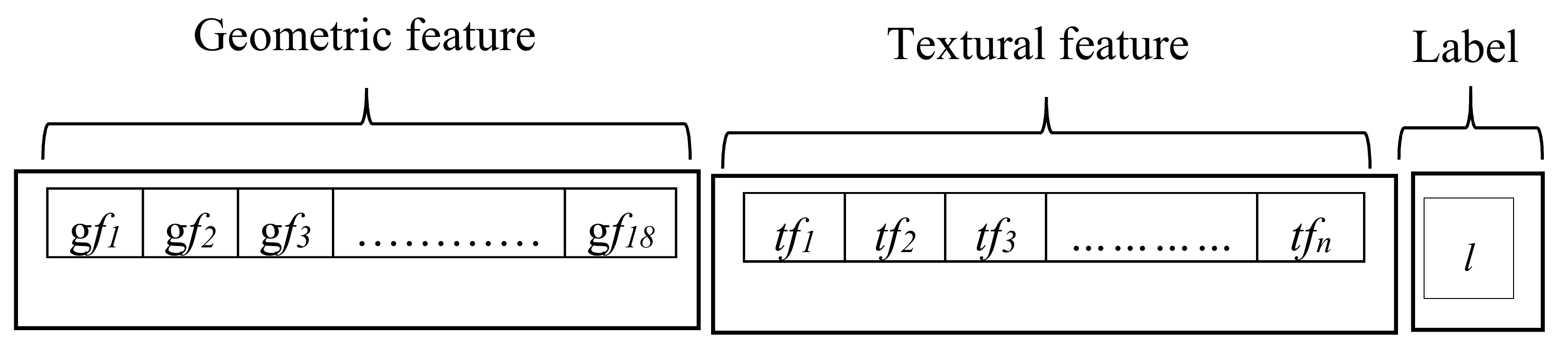
3.2. Feature Extraction

In this section, the extraction of two types of features—namely, geometric and texture features—is explained.

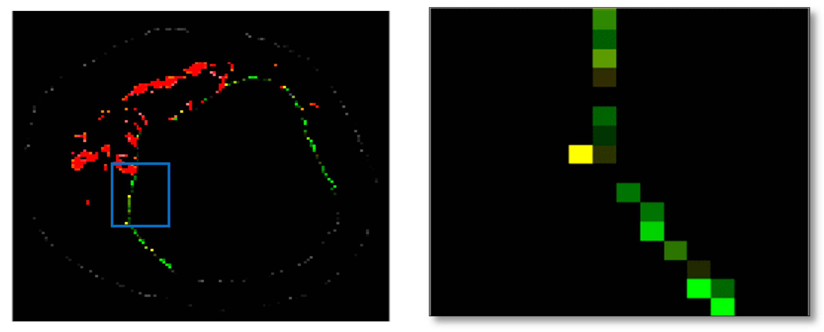
3.2.1. Geometric-Based Features

Geometric features consist of tissue area, luminal border, and plaque component features. With regard to our previous work [45], the Close Lumen Border Tracing (CLBT) and Open Lumen Border Tracing (OLBT) algorithms trace the luminal border. The results for the lumen border obtained by the CLBT and OLBT algorithms are a sequence of n elements. To extract the luminal border features, the intensity value of each member is extracted. The amount of NC in contact with the lumen (f_NCCL) and DC in contact with the lumen (f_DCCL) are calculated based on the number of red and white pixels in the lumen border. To extract the plaque component features, three algorithms, including Extracting Confluent Components (ECC), Necrotic Core Layering (NCL), and Plaque Burden Assessment (PBA), are applied. The ECC algorithm extracts the confluent components, including the Confluent NC (CNC) and the Confluent DC (CDC). The DC images which do not belong to the CDC are considered to be Micro Calcification (MicroCa). The NC images which do not belong to the CNC are considered to be Scattered Necrotic Core (SNC). Furthermore, confluent NC in contact with the lumen (CNCCL) and confluent DC in contact with the lumen (CDCCL) are calculated. The area of CNC, CDC, MicroCa, SNC, CNCCL, and CDCCL are calculated as f_CNC, f_CDC, f_MicroCa, f_SNC, f_CNCCL, and f_CDCCL, respectively.

TCFA is categorised into two classes: single and multiple confluent NC layers [78]. The NCL algorithm determines the NC layering (f_NCL) and DC layering (f_DCL). Quantifying the plaque burden is crucial in terms of diagnosing vulnerable plaque [79]. Therefore, the PBA algorithm measures the plaque burden features, including plaque area (f_PA), vessel area (f_VA), lumen area (f_LA), and plaque burden (f_PB). Therefore, each VH-IVUS image has three different types of geometric feature: tissue plaque area, luminal border, and plaque component features referred to as geometric features GF = {f_NC, f_DC, f_FI, f_FF, f_NCCL, f_DCCL, f_CNC, f_SNC, f_CDC, f_MicroCa, f_CNCCL, f_CDCCL, f_NCL, f_DCL, f_PA, f_VA, f_LA, f_PB}_ENREF_1_ENREF_1.

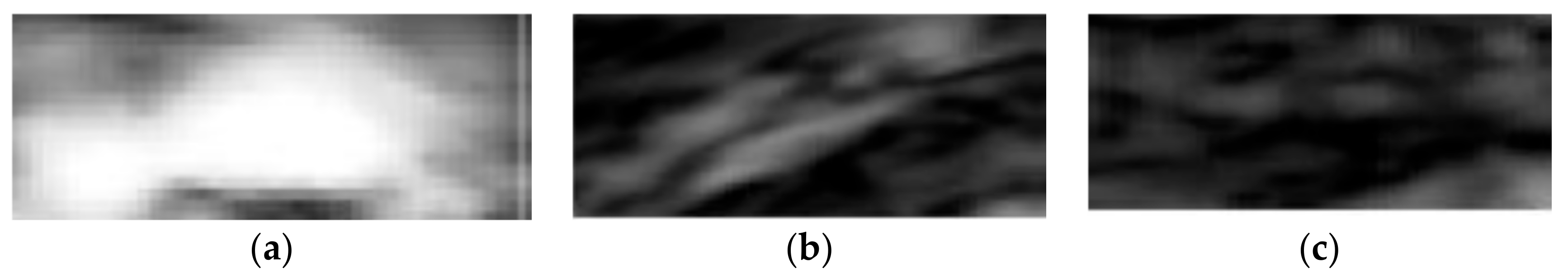
3.2.2. Texture-Based Features

Biomedical texture operations analyse the desired texture information in terms of spatial scales and the directions of a texture image, which are fundamental for visual texture discrimination. The most important characteristic of texture is that it is scale dependent [80]. Due to the fact that pixel-based grey-level-only methods are not sufficient to discriminate the complicated structures of tissue components, texture features are used [81]. It is an important and challenging problem to extract the desirable feature set for the classification step [56]. Texture features are widely used for analysing medical images. Texture is a primary visual feature, referring to the natural properties of the object in the image [82]. This approach analyses the spatial variations of pixel intensities and quantifies them into a numerical value [83,84]. In addition to geometric features, which depend on pixel intensity, texture-based approaches characterise the statistical and spatial relationships in the neighbourhood of the pixel [82]. Since geometrical features are often local in nature, the spatial information of the image will not be considered [15]. Therefore, texture features, as a global pattern, are defined to analyse the micro textures [16].

Low-level quantitative image analysis can be categorised based on intensity and texture. Image intensity describes the statistical distribution of the pixel values inside a Region of Interest (ROI) [80]. Many forms of texture analysis have been developed, including co-occurrence matrices, second-order statistics, Gauss–Markov random field, etc. These methods were limited to the analysis of spatial relations within small neighbourhoods and the analysis of micro textures [16]. However, texture information relates to the micro- and macro-structural context of biomedical tissue [80]. Classic examples of texture operators such as Gabor wavelets, GLCMs, Histogram of Oriented Gradients (HOG), LBPs, and Scattering Transforms (ST) need to be able to discriminate between types of image scales, directions, and transitions. Designing an ideal set of texture operators that is able to accurately identify the tissue type is a very challenging task. However, the comprehensive analysis of spatial scales and directions is computationally expensive for discrete texture functions. Therefore, combinations of image scales and directions with discriminative capabilities for each plaque component should be considered. If the descriptor is insensitive to the transformation of the input image, the operator is invariant [80].

Previous studies have identified texture analysis as being useful in the analysis of ultrasound images. Plaque components appear with different texture patterns in IVUS images (Figure 11). Therefore, texture analysis methods are best suited to classifying pixels from plaque areas of IVUS images into three tissue classes, including dense calcium (DC), necrotic core (NC), and fibro-fatty (FF) [47].

Before extracting the texture features, it should be emphasised that some descriptors for texture classification could be used, such as Gabor filters, Hidden Markov trees, or the wavelet approach [85]. However, the effective classification of plaque type involves the generation of significant features. These discriminative features will be combined with geometric features as input data for the classifier. Such choices can made on the basis of a study of the literature.

Grey-Level-based texture descriptors can be designed to reflect the different grey-level profile characteristics of the hard and soft plaque. Co-occurrence matrices describe the repeated occurrences of some grey-level configurations in the plaque texture classes. Run-length measures describe the maximum contiguous set of constant grey-level pixels located in a specified direction. A large number of neighbouring pixels of the same grey level represents a coarse texture, while a small number of these pixels represents a fine texture. Some microstructures of binary patterns in images can be detected by LBP [47]. According to the adapted algorithm by Taki [47], a higher overall accuracy was achieved by co-occurrence and LBP methods for characterising the fibro-lipid regions. Moreover, the run-length feature indicated a better capability for classifying DC plaques, while LBP and co-occurrence exhibited a better performance for NC. Texture descriptors such as LBP and MRL may miss useful information in grey levels of IVUS images, so grey-level information in combination with LBP and MRL features were employed to better classify the plaque types [20]. Because the best results on IVUS tissue characterisation were achieved using LBP, GLCM, and MRL, these three sets of features were used for the texture descriptor from the VH-IVUS images using the same data set.. These methods are explained in the following sub sections.

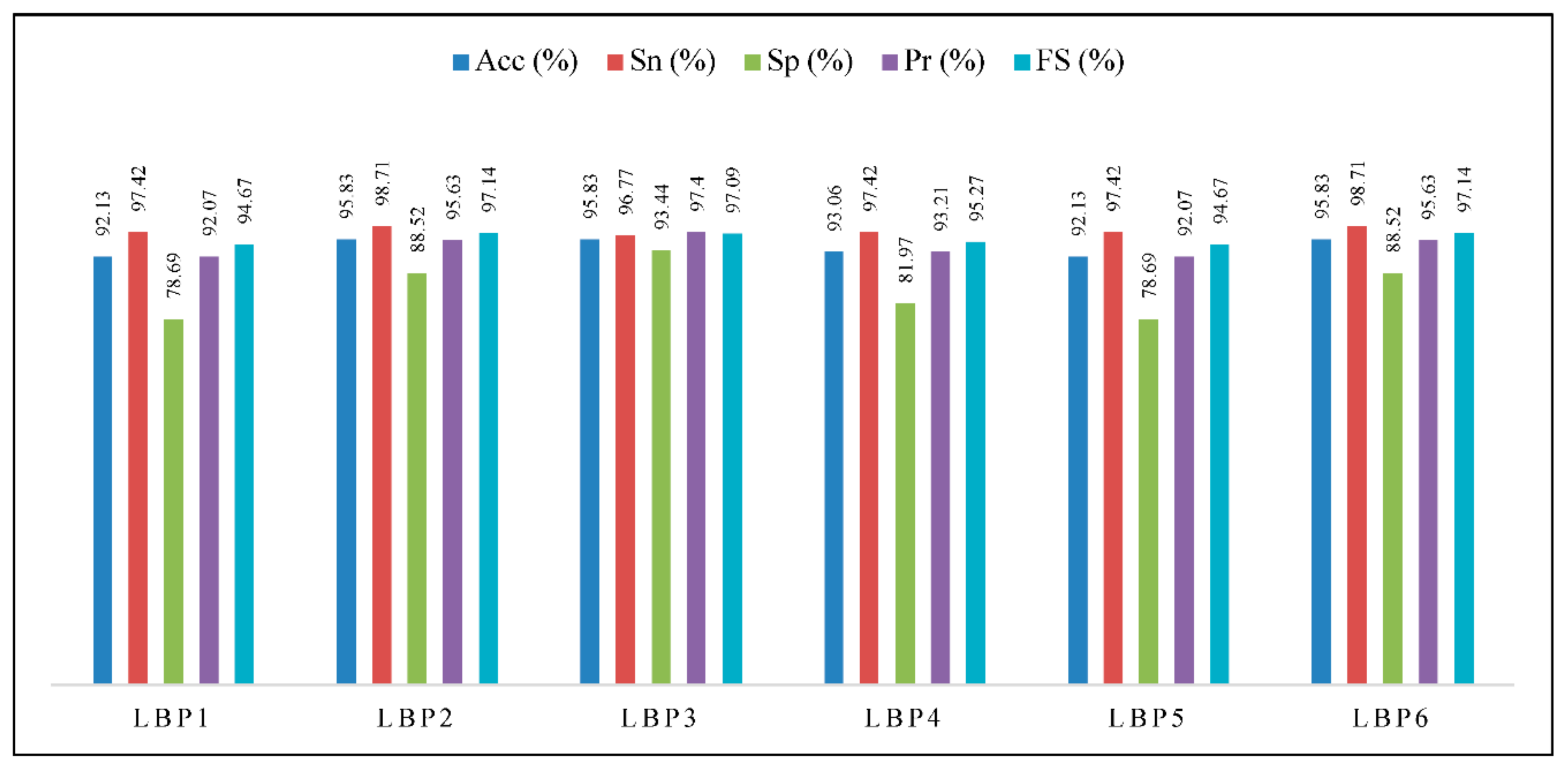
3.2.3. Local Binary Patterns (LBP)

The LBP technique proposed by Ojala et al. [86] is a robust and efficient classical type of textural descriptor for a wide range of applications [87]. Due to its computational simplicity, it is possible to analyse the images in real-time applications [88]. Also, by applying a non-overlap window, LBP considerably reduces the image matrix without losing the texture information [88]. In this method, the relationships between a pixel and its local neighbours are defined by a “local pattern”. Consider P to indicate the circular neighbourhood pixel on a circle of radius R. Let G_c represent the grey value of the centre pixel and Gp indicate the grey value of the neighbourhood pixels for p = 0, 1,…, p − 1. Based on the local structure around the centre pixel, circular points can be represented as 8-bit binary codes [87]. The local texture is defined by:

$$\mathrm{T}=\mathrm{t}\left({\mathrm{G}}_{\mathrm{c}},{\mathrm{G}}_0,\dots ,{\mathrm{G}}_{\mathrm{P}-1}\right)$$

(8)

The LBP of centre pixel is obtained by the following equation:

$$LB{P}_{P,R}={{\displaystyle \sum }}_{p=0}^{P-1}F\left(G_p-G_c\right)2^p$$

(9)

where

$$F\left(x\right)=\{\begin{array}{cc}1,& x\le 0\\ 0,& otherwise\end{array}$$

(10)

The LBP_P,R is calculated by subtracting the centre pixel from its neighbours [87].

3.2.4. Grey Level Co-Occurrence Matrix (GLCM)

Haralick et al. [89] presented the GLCM and textural features for image classification. GLCM matrix depicts the occurrence of two adjacent pixels with grey values of i and j. For an M × N image, GLCM is defined based on the following equation [90]:

$$C_d\left(i,j\right)=\left|\left\{\begin{array}{cc}\left(p,q\right),& \left(p+\Delta x,q+\Delta y\right):I\left(p,q\right)=i,\\ & I\left(p+\Delta x,q+\Delta y\right)=j\end{array}\right\}\right|$$

(11)

where $\left(p,q\right), \left(p+\Delta x,q+\Delta y\right) \in M\times N, d=\left(\Delta x,\Delta y\right)$ and |.| represents the cardinality of a defined set. For a grey level i, the probability of the grey level j with distance d is obtained by the following equation:

$$P_d\left(i,j\right)=\frac{C_d\left(i,j\right)}{\sum C_d\left(i,j\right)}$$

(12)

The matrix element P (i, j| d, θ) indicates the probability values for changes between grey levels ‘i’ and ‘j’, while d is the distance between pixels and θ depicts the particular angle between the neighbours. Typically, d = 1,2 and the orientations θ = 0°, 45°, 90°, 135° are calculated [15].

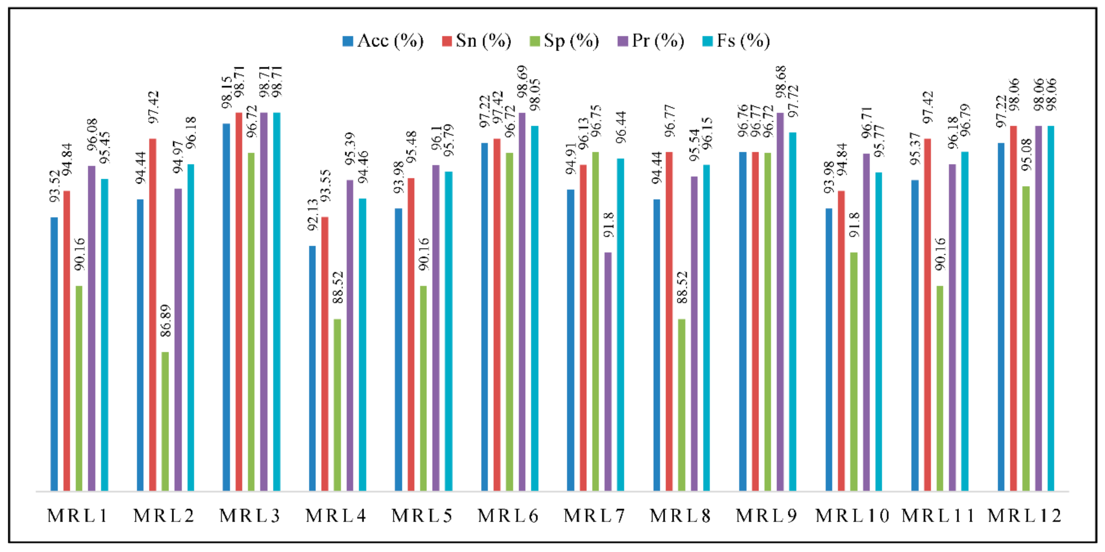
3.2.5. Modified Run Length Matrix (MRL)

RL statistics extract higher-order statistical features in terms of specified directions [91]. The RL method captures the coarseness of a texture in the specified directions. For a given image, a run-length matrix P involves p(i,j) elements to define the number of runs of length j with pixels of grey level i [92]. Calculating the run-length while encoding for each typical orientation produces four run-length matrices [19]. The typical orientations are 0°, 45°, 90°, and 135°.

3.2.6. Feature Selection

To obtain an effective and discriminating feature set and to reduce the redundancy of the feature space, feature selection can be performed [56]. Therefore, Principle Component Analysis (PCA) is applied to reduce the dimensionality of the texture features and to obtain informative features [90]. The first row of the obtained matrix is selected as the first principle components of PCA. Since some of the acquired features often have very small values compared to others, a normalisation process [93] is needed. Therefore, features are normalised using the zscore function (i.e., mean centring with a unit standard deviation constraint) [94].

3.3. Classification

3.3.1. Machine Learning Algorithms

To select the appropriate classifier, various factors should be considered, including computational cost, classification accuracy for several datasets, and performance [15]. The well-known classification approaches k-NN, SVM, and ANNs were developed specifically to deal with uncertain data. These methods provide a probability measure in order to classify samples with different class memberships [95]. Therefore, in this study, the three most common classifiers—SVM, ANN, and kNN—are employed.

The SVM classifier usually outperforms other soft-computing approaches in terms of efficiency, scalability, and performance [96]. SVM is rather insensitive to feature correlation and is typically adopted to handle high-dimensional feature spaces [87]. This classifier minimises the number of misclassifications. However, the training time is very high [56]. Also, the provided kernel matrix of input samples must be stored in its memory. The desired optimal solution for non-linear mapping depends on selecting an appropriate kernel function as well [52].

It has been reported that the Artificial Neural Network (ANN) performs very well on complicated data, noisy fields, and multivariate nonlinear domains [56]. ANN demonstrates complex global behaviour to provide the desired outputs in a supervised or unsupervised manner [97]. One basic feature that distinguishes this method from an algorithmic program is the ability to classify unseen data [98]. Additionally, the potential of nonlinear mapping increases the flexibility of the ANN method for modelling complex relationships [56]. However, due to the use of gradient methods in the learning process, ANN is very time consuming [56]. Iteration number, learning rate, and activation function affect the accuracy rate of ANN as well [99].

K-NN is a very simple algorithm. Therefore, its implementation and debugging are relatively easy. This algorithm searches the training set to select the k nearest neighbours of the unseen features and estimates their class label based on the majority voting technique. K-NN can be used for large numbers of training sets. However, its classification and estimation are moderately slow. Additionally, the choice of k affects the performance of this algorithm. Moreover, the accuracy of this algorithm may be degraded in the presence of noisy or irrelevant features [56].

3.3.2. Evaluation

K-Fold Cross Validation

The most extensively used validation method is the sub sampling test (k-fold cross validation). To evaluate the performance of classifiers, this method divides the dataset into N equivalent blocks, whereas N − 1 blocks are often employed as training and the rest is used for testing. To evaluate the performance, the mean value is frequently measured after repetition of several rounds. Moreover, tests can be repeated several times to obtain reliable results. 10-fold and 5-fold cross validation have been used extensively [100].

Performance Measures

Performance measures are defined using the “confusion matrix” illustrated in

Table 4. Confusion matrix.

Class	Classified as Positive	Classified as Negative
+	TP: The number of correctly predicted positives.	FN: The number of incorrectly predicted negatives.
−	FP: The number of incorrectly predicted positives.	TN: The number of correctly predicted negatives.

, including TP (True Positive), FN (False Negative), FP (False Positive), and TN (True Negative) [101,102].

To validate the consistency of the proposed model, statistical measures have been applied, including accuracy, precision, sensitivity (recall), specificity, and F-Score based on the following equations:

$$Accuracy=\frac{TP+TN}{TP+TN+FP+FN}$$

(13)

$$\mathrm{Precision}=\frac{TP}{\left(TP+FP\right)}$$

(14)

$$Recall=\frac{TP}{TP+FN}$$

(15)

$$Specificity=\frac{TN}{TN+FP}$$

(16)

$$F-score=\frac{2\times Precision\times Recall}{Precision+Recall}$$

(17)

3.3.3. TCFA Detection Using Geometric Features

Since TCFA detection involves subjective assessment [103], developing a comprehensive and automatic method for classification of plaque type using machine learning algorithms is essential. Inter-observer variability in the diagnosis of vulnerable plaque can be minimised by applying classification methods [54]. Geometric feature vectors extracted from all VH-IVUS images in the data set were horizontally concatenated to construct a feature matrix called FM of size 588 × 18, where 588 indicates the number of VH-IVUS images and 18 the number of geometric features. Regarding the given criteria for TCFA, each row in the FM matrix is assigned a label of ‘1’ or ‘0’ to indicate the TCFA and non-TCFA, respectively. Therefore, 81 feature vectors were assigned as TCFA and 507 feature vectors were labelled as non-TCFA plaque. The assigned labels were attached at the end of each feature vector.

FM is divided into two matrices, namely, FM_Train (70%) and FM_Test (30%). FM_Train is used to build the model, while FM_Test is applied to validate the model. In each validation step, FM_Train is divided into five equal parts, consisting of four parts for the training data set and a fifth part for the testing data. This procedure is repeated five times, each time with a new part as test vector [91]. Each five-fold cross validation is run on FM_Train ten times. Finally, the averages of sensitivity, specificity, and accuracy derived from 50 runs are reported as the total result of the classifier [104].

In this section, different combinations of extracted features are examined to find the best technique for identifying TCFA plaque. Therefore, multiple classifiers, including the Back Propagation Neural Network (BPNN), kNN, and SVM, are examined to classify the plaque type into TFCA and non-TCFA. To achieve higher performance of SVM, FM_Train is fed to the SVM classifier with linear, polynomial kernel functions in the order 1, 2, and 3, and Radial Basis Function (RBF) with different sigma values [69]. Different k values are applied to investigate the performance of k-NN classifier, as well [105]. The results in terms of accuracy (Acc), sensitivity (Sn), specificity (Sp), precision (Pr), and F-score (FS) are illustrated in

Table 5. Performance of multiple classifiers using geometrical features (Acc: accuracy, Sn: sensitivity, Sp: specificity, Pr: precision, and FS: F-score).

Classifiers	Acc (%)	Sn (%)	Sp (%)	Pr (%)	FS (%)
BPNN	87.04	98.91	18.75	87.50	92.86
KNN_5	95.37	98.37	78.13	96.28	97.31
KNN_10	92.59	97.83	62.50	93.75	95.74
KNN_15	93.06	96.20	75.00	95.68	95.94
KNN_20	87.50	96.74	34.38	89.45	92.95
KNN_25	88.43	97.83	34.38	89.55	93.51
KNN_30	88.43	97.83	34.38	89.55	93.51
SVM_MLP	82.87	85.81	75.41	89.86	87.79
SVM_Linear	95.83	96.77	93.44	97.40	97.09
SVM_Poly_1	96.71	98.71	91.80	96.84	97.76
SVM_Poly_2	96.76	97.42	95.08	98.05	97.73
SVM_Poly_3	97.69	99.35	93.44	97.47	98.40
SVM_rbf_0.80	95.83	98.71	88.52	95.63	97.14
SVM_rbf_0.90	96.76	99.35	90.16	96.25	97.78
SVM_rbf_1	95.83	98.06	90.16	96.20	97.12
SVM_rbf_1.10	97.69	100	91.80	96.88	98.41
SVM_rbf_1.20	97.22	98.06	95.08	98.06	98.06

.

As illustrated in Table 5, the best result in terms of accuracy was obtained when SVM_Poly_3 and SVM_rbf _1.10 were applied, whereas the worst result was obtained for the SVM_MLP. On the other hand, SVM_rbf _1.10 and SVM_MLP demonstrated the best and the worst results, respectively, in terms of sensitivity. Furthermore, the best result in terms of specificity was obtained when SVM_Poly _2 and SVM_rbf_1.20 were used, whereas the worst result was obtained for the BPNN. Moreover, SVM_rbf_1.20 and BPNN showed the best and the worst results in terms of precision. Furthermore, the best results in terms of F-score were obtained when SVM_rbf _1.10 was applied, whereas the worst result was obtained for the SVM_MLP.

Figure 12 illustrates the accuracy of multiple classifiers obtained based on geometric features. SVM_rbf_1.10 and SVM_Poly_3 achieved the best result for accuracy; therefore, they were selected to perform the TCFA detection using combined features.

3.3.4. TCFA Detection Using Geometric and Texture Features

In this section, classification was performed using geometric and texture features. The geometric and texture features were concatenated horizontally to carry out the plaque classification.

Table 6. Texture feature description.

Feature	Description
GF_LBP	Combined geometric and LBP features.
GF_LBP_PCA	Combined geometric and the first principle components of LBP
GF_GLCM	Combined geometric and GLCM features.
GF_GLCM_PCA	Combined geometric and first principle components of GLCM
GF_MRL	Combined geometric and MRL features.
GF_MRL_PCA	Combined geometric and the first principle components of MRL

illustrates the descriptions of the texture features.

All experiments were conducted by applying the SVM_rbf_1.10. The following sub sections describe the experiments and analyses that were carried out for combined features. To investigate the power of texture features for TCFA detection, combined features were obtained by concatenating the texture features with the geometric features. The label of each geometric feature vector that was attached at the end of this vector must be moved to the end of the new feature vector. For every VH-IVUS image, geometric features (GF) and texture features (TF) were extracted. Figure 13 demonstrates the combined features using geometric and texture features.

Combination of Geometric and LBP Features

LBP features were extracted from VH-IVUS image for two different sets of P and R ((8, 1) and (16, 2)). Then, features of two vectors of size 1 × 256 and 1 × 65,536 were obtained for LBP_8,1 and LBP_16,2, respectively. The PCA technique was then applied, and the first component was selected for each feature set. Therefore, LBP and the geometric features consisted of 6 members: LBP_8,1 (LBP₁), GF_LBP_8,1 (LBP₂), GF_LBP_8,1_PCA (LBP₃), LBP_16,2 (LBP₄), GF_LBP_16,1 (LBP₅), GF_LBP_16,1_PCA (LBP₆). Performance measurements were obtained on the basis of accuracy, sensitivity, specificity, precision, and F-score. Figure 14 illustrates the results of the SVM classifier using geometrical and LBP features.

As depicted in Figure 14, the best accuracy results were achieved by LBP₂, LBP₃, and LBP₆, while the worst results were obtained by LBP₁ and LBP₅. In addition, the best results for sensitivity were provided by LBP₂ and LBP₆, whereas the worst result was obtained by LBP₃. However, LBP₃ obtained the best results for specificity and precision. The feature sets LBP₂ and LBP₆ provided the best results in terms of F-score. Meanwhile, LBP₁, LBP₅ provided the lowest values of specificity, precision, and F-score.

Combination of Geometric and GLCM Features

GLCM algorithms were applied to detect the uniform texture patterns of VH-IVUS images with angles of 0, 45, 90, and 135. Therefore, GLCM₀, GLCM₄₅, GLCM₉₀, and GLCM₁₃₅, with size 1 × 20, were created. The first component of PCA was also selected for each feature set, so four additional feature sets were generated. Therefore, GLCM and geometric features consisted of 12 members: GLCM₀ (GLCM₁), GF_GLCM₀ (GLCM₂), GF_GLCM₀_PCA (GLCM₃), GLCM₄₅ (GLCM₄), GF_GLCM₄₅ (GLCM₅), GF_GLCM₄₅_PCA (GLCM₆), GLCM₉₀ (GLCM₇), GF_GLCM₉₀ (GLCM₈), GF_GLCM₉₀_PCA (GLCM₉), GLCM₁₃₅ (GLCM₁₀), GF_GLCM₁₃₅ (GLCM₁₁), GF_GLCM₁₃₅_PCA (GLCM₁₂). Figure 15 illustrates the results of SVM using a combination of geometric and GLCM features.

As illustrated in Figure 15, GLCM₆ achieved the best results in terms of accuracy and sensitivity, whereas GLCM₁₁ achieved the worst results for accuracy and sensitivity. In addition, GLCM₉ achieved the best results in terms of accuracy, specificity, precision, and F-score. GLCM₅ and GLCM₈ obtained the worst results for specificity and precision. GLCM₁₁ achieved the worst result for F-score. The experimental results demonstrated that feature selection increased the classification accuracy.

Combination of Geometric and MRL Features

In this section, a combination of geometric and MRL features is explored. To extract the MRL features, the VH-IVUS image is taken as a region. MRL feature combination with angles 0, 45, 90, and 135 was performed, and four feature vectors of size 1 × 11 were obtained. The PCA algorithm was applied for dimension reduction, and then the first component was selected for each feature set. Therefore, the MRL and geometric features consisted of 12 members: MRL₀ (MRL₁), GF_MRL₀ (MRL₂), GF_MRL₀_PCA (MRL₃), MRL₄₅ (MRL₄), MRL₄₅ (MRL₄), GF_MRL₄₅ (MRL₅), GF_MRL₄₅_PCA (MRL₆), MRL₉₀ (MRL₇), GF_MRL₉₀ (MRL₈), GF_MRL₉₀_PCA (MRL₉), MRL₁₃₅ (MRL₁₀), GF_MRL₁₃₅ (MRL₁₁), GF_MRL₁₃₅_PCA (MRL₁₂). The SVM classifier was employed to classify the different combination of GF and MRL feature sets. Figure 16 depicts the results of SVM classification using a combination of geometric and MRL features with angles 0, 45, 90, and 135.

As demonstrated in this figure, the best performance in terms of accuracy, sensitivity, precision, and F-score was achieved by applying MRL₃, but the best result for sensitivity was obtained by MRL₇. However, MRL₄ provided the lowest accuracy and sensitivity results. Moreover, MRL₂, MRL₇, and MRL₄ obtained the worst results in terms of specificity, precision, and F-score, respectively. Figure 17 illustrates the best accuracy of geometric and texture features. With regard to this figure, combined geometric and GLCM features achieved the best accuracy.

4. Validation

Although a few program-based studies have been developed to extract features from VH-IVUS images and to diagnose TCFA, a comprehensive method to investigate the strengths and weaknesses of the proposed methodology is needed. This section presents the validation and effectiveness of the proposed approach. To evaluate the quality of the automatic classification, three different experiments were conducted [45]. In the first experiment, validation was carried out based on the presence of the TCFA plaque in Optical Coherence Tomography (OCT) images. In the second experiment, validation was conducted based on the class labels provided by SVM and labels that were manually defined based on a cardiologist’s decision for 58 VH-IVUS and their corresponding IVUS images. In the last experiment, the results of SVM and cardiologist decision were compared for 76 VH-IVUS images.

4.1. Validation by OCT

TCFA plaque is characterised by a necrotic core with an overlying thin fibrous cap (<65 µm). The principal difficulty with diagnosis of the TCFA lesions with IVUS modality is the limited axial resolution (approximately 150 µm). Therefore, IVUS-based technology is unable to visualise the thin fibrous caps [30]. This modality is presented as the in-vivo “gold standard” for measuring the fibrous cap thickness for diagnosis of TCFAs [106]. By means of the validated criteria for plaque characterisation, the minimum fibrous cap thickness is measured at the minimum luminal area site in OCT images [107]. To validate TCFA plaque, VH-IVUS images can be compared to their corresponding OCT image. Plaques are classified into TCFAs and non-TCFAs based on the fibrous cap thickness in OCT.

In this experiment, 18 geometric features were extracted from 14 VH-IVUS images, which were provided by Kermani et al. [108]. The SVM classifier with a RBF kernel was then applied to classify each feature vector into TCFA and non-TCFA plaques. These images were then labelled based on their corresponding OCT images using the proposed method by Kermani, Ayatollahi and Taki [108]. In this manner, TCFA was extracted from the corresponding OCT frames. If TCFA exists in those OCT frames, ‘1’ is assigned; otherwise, ‘0’ is assigned, to represent non-TCFA plaque. Based on the results, SVM classifies the VH-IVUS images into 2 TCFA and 11 non-TCFA plaques; meanwhile, the OCT-based method classifies the data into 3 TCFA and 10 non-TCFA plaques. The confusion matrix was then calculated, and the performance measures were presented in terms of true positive (TP), true negative (TN), false positive (FP), false negative (FN), accuracy, sensitivity, specificity, precision, and F-score.

Table 7. Diagnostic accuracy of VH-IVUS to detect TCFA as determined by OCT.

TP	TN	FP	FN	Accuracy	Sensitivity	Specificity	Precision	F-Score
11	2	0	1	92.85%	91.67%	100%	100%	95.65%

depicts the diagnostic accuracy of VH-IVUS for detecting TCFA as determined by OCT.

Based on the above table, TP and TN demonstrate that VH-IVUS correctly identified 11 non-TCFA and 2 TCFA plaques. In addition, FP represents that all non-TCFA plaque was correctly classified, whereas FN indicates that VH-IVUS misclassified 1 TCFA plaque, as determined by OCT. Furthermore, VH-IVUS demonstrates an acceptable result in terms of accuracy, sensitivity, specificity, precision, and F-score to identify TCFA as determined by OCT.

4.2. Validation Using VH-IVUS and IVUS Images

For this experiment, 58 VH-IVUS and their corresponding IVUS were selected from three patients. VH-IVUS images are classified into TCFA and non-TCFA based on the SVM classifier, cardiologist decision, and the presented algorithm by Calvert et al. [109]. TCFA was identified based on its having a plaque burden > 40%, confluent necrotic core > 10% of plaque cross-sectional area in contact with vessel lumen for 3 consecutive frames [109].

Table 7 illustrates the comparison between CA, SVM, and CD methods for TCFA detection. Columns CA, SVM, and CD indicate the results of the implemented algorithm by Calvert, Obaid, O’Sullivan, Shapiro, McNab, Densem, Schofield, Braganza, Clarke and Ray [109], SVM with RBF kernel, and cardiologist decision, respectively. The TCFA plaques are labelled with ‘1’ and the non-TFCAs are represented with ‘0’. The number of detected TCFA by CA, SVM, and CD methods was 18, 16, and 11 images, respectively. Based on the assigned labels, the confusion matrix is obtained, and TP, TN, FP, FN, accuracy, sensitivity, specificity, precision, and F-score are presented in

Table 8. Comparison between CA, SVM, and CD methods for TCFA detection (TP: true positive, FP: false positive, FN: false negative, TN: true negative).

Method	TP	TN	FP	FN	Accuracy	Sensitivity	Specificity	Precision	F-Score
CA&CD	9	38	2	9	81.03	50	95	81.81	62.07
CA&SVM	11	35	5	7	79.31	61.11	87.50	68.75	64.70
CD&SVM	8	39	3	8	81.03	84.81	84.81	84.81	75.78

.

Based on Table 8, CA&SVM and CD&SVM provide the maximum number of correctly identified non-TCFA and TCFA plaques, respectively, while CD&SVM and CA&SVM obtain the minimum number of correctly identified non-TCFA and TCFA plaques respectively. Furthermore, the highest numbers of misclassified non-TCFA and TCFA plaques were provided by CA&SVM and CA&CD, while, CA&CD and CA&SVM generated the lowest number of misclassified non-TCFA and TCFA plaques, respectively. Moreover, CD&SVM achieved the best results in terms of accuracy, sensitivity, precision, and F-score. The best results for accuracy and specificity were obtained by CA&CD, as well, while CA&SVM achieved the worst results in terms of accuracy and precision. In addition, CA&CD provided the lowest values of sensitivity and F-score and CD&SVM received the lowest value for specificity.

4.3. Validation Using VH-IVUS Images

For this experiment, 76 VH-IVUS images were selected from five patients. The VH-IVUS images were classified into TCFA (‘1’) and non-TCFA (‘0’) by SVM with RBF kernel. A cardiologist’s decision was also applied, and those images were classified [109]. Based on the assigned labels, a confusion matrix was obtained and TP, TN, FP, FN, accuracy, sensitivity, specificity, precision, and F-score are presented in

Table 9. Diagnostic accuracy of VH-IVUS for detecting TCFA based on cardiologist decision and SVM (TP: true positive, FP: false positive, FN: false negative, TN: true negative).

TP	TN	FP	FN	Accuracy	Sensitivity	Specificity	Precision	F-Score
41	33	0	2	97.36	95.34	100	100	97.61

.

Based on the above table, TP and TN demonstrate that VH-IVUS correctly identified 41 non-TCFA and 33 TCFA plaques. In addition, FP indicates that all non-TCFA plaques are correctly classified, whereas FN depicts that VH-IVUS misclassified two TCFA plaques. Furthermore, VH-IVUS demonstrates acceptable results in terms of accuracy, sensitivity, specificity, precision, and F-score in identifying TCFA plaque. The accuracy of the cardiologist’s decision and the SVM classifier for 76 VH-IVUS images achieved the best results, with 97.36% in terms of accuracy. These results demonstrate that the proposed approach has the potential to identify high-risk lesions.

5. Discussion

Spectrum analysis of IVUS-derived radiofrequency (RF) data enables a more detailed analysis of plaque morphology. Preliminary in vitro studies correlated four histological plaque components with a specific spectrum analysis of the RF data. The different components, consisting of fibrous, fibrofatty, necrotic core, and dense calcium, were colour coded. Coronary tissue maps were reconstructed from RF data using VH-IVUS software. VH- IVUS has the potential to detect high-risk lesions and can provide new insights into the pathophysiology of coronary artery disease [110]. However, the overlapping tissue in VH-IVUS image causes difficulty in segmentation of atherosclerotic plaques [29]. Simple clustering methods based on the pixels’ intensities are not reliable for segmenting the highly mixed tissue types involved in VH-IVUS images. To overcome this limitation, robust semi-supervised models were presented in this study. The main contribution of this paper is proposing the KMPSO-mED classification methodology based on semi-supervised learning theory to improve the accuracy of VH-IVUS image segmentation. This model does not require a training sample, and as a result, time and resources can be saved. Therefore, it improves the accuracy of pixel classification when sufficient training data are not available. It classifies the test image without any prior information regarding the number of clusters. The proposed model has the potential to discriminate overlapping tissue. The segmentation process was moderately fast due to the pixel-wise classification. The designed models attempt to take advantage of supervised learning in the segmentation of test images. These models can also enhance the ability of the clustering algorithm by removing outliers to provide more accurate segmentation results in the VH-IVUS image. Furthermore, these techniques are capable of dividing the clusters with different densities in the VH-IVUS image.

In medical diagnosis, misclassifying plaque tissue as vulnerable plaque could be highly important. Plaque components consisting of NC, DC, FF, and FI have different textures in IVUS-based images [26]. To capture the varying heterogeneity of plaque components, multi-scale feature extraction is applied. Another novelty of the proposed method is that it is a linear combination of geometric and informative texture features to compute a discriminative index for plaque classification and TCFA detection. The present study proposes a computer-aided method for plaque type classification that is fast and accurate. To provide the correct classification, a fusion of different geometric and texture features has been applied, whereas existing research on TCFA detection has only focused on the geometric features. Nevertheless, it takes more time to extract the texture features and feature selection; also, the range of values of the geometric and texture features are different, and this affects the classification accuracy in fusion step.

An automatic classification approach is required to reduce observer error; also, the accuracy will not be affected by the characterisation of a large number of medical images [111]. To emphasise the significance of the feature fusion technique, the SVM classifier is compared with individual texture models based on accuracy, sensitivity, and specificity measurements. In comparison with LBP, GLCM, and MRL, the combined feature sets exhibited better classification accuracy. With regard to the results, the best classification accuracy was obtained by combining the first principle components of GLCM and geometric features. For future work, other descriptors of texture classification could be used, such as Gabor filters, Hidden Markov trees or the wavelets approach. Moreover, a convolutional neural network (CNN) model will be applied to classify the plaque type into TCFA and non-TCFA. The proposed approach can further be extended to define the vulnerability index as ‘low’, ‘moderate’, ‘severe’, and ‘very severe’.

6. Conclusions

In this paper, segmentation approaches consisting of FCMPSO-mED and KMPSO-mED have been developed in order to specify the spatial intra-plaque distribution of VH–IVUS components. Furthermore, three commonly used statistical methods, including LBP, GLCM, and MRL, are presented to extract the texture features. Based on the experiments, the best performance of classification was achieved by applying the combined plaque and texture features. The experimental results proved the superiority of the proposed method, with a high accuracy rate of 98.61% for the diagnosis of TCFA plaque.

References

1. Sun, S. An innovative intelligent system based on automatic diagnostic feature extraction for diagnosing heart diseases. Knowl.-Based Syst. 2015, 75, 224–238. [Google Scholar] [CrossRef]
2. Konig, A.; Bleie, O.; Rieber, J.; Jung, P.; Schiele, T.M.; Sohn, H.Y.; Leibig, M.; Siebert, U.; Klauss, V. Intravascular ultrasound radiofrequency analysis of the lesion segment profile in ACS patients. Clin. Res. Cardiol. 2010, 99, 83–91. [Google Scholar] [CrossRef] [PubMed]
3. Brown, A.J.; Obaid, D.R.; Costopoulos, C.; Parker, R.A.; Calvert, P.A.; Teng, Z.; Hoole, S.P.; West, N.E.; Goddard, M.; Bennett, M.R. Direct comparison of virtual-histology intravascular ultrasound and optical coherence tomography imaging for identification of thin-cap fibroatheroma. Circ. Cardiovasc. Imaging 2015, 8, e003487. [Google Scholar] [PubMed]
4. Cascón-Pérez, J.D.; de la Torre-Hernández, J.M.; Ruiz-Abellón, M.C.; Martínez-Pascual, M.; Mármol-Lozano, R.; López-Candel, J.; Cano, P.; Fernández, C.; Ramos, J.L.; Villegas, M. Characteristics of culprit atheromatous plaques obtained in vivo by intravascular ultrasound radiofrequency analysis: Results from the CULPLAC study. Am. Heart J. 2013, 165, 400–407. [Google Scholar] [CrossRef] [PubMed]
5. Liang, M.; Puri, A.; Devlin, G. The vulnerable plaque: The real villain in acute coronary syndromes. Open Cardiovasc. Med. J. 2011, 5, 123–129. [Google Scholar] [CrossRef] [PubMed]
6. Akasaka, T.; Kubo, T. Identification of Vulnerable Plaques with Optical Coherence Tomography. In Atherosclerotic Cardiovascular Disease; Pesek, D.K., Ed.; InTech: Tokyo, Japan, 2011. [Google Scholar] [Green Version]
7. Escalera, S.; Pujol, O.; Mauri, J.; Radeva, P. Intravascular ultrasound tissue characterization with sub-class error-correcting output codes. J. Signal Process. Syst. 2009, 55, 35–47. [Google Scholar] [CrossRef]
8. Zhu, X.; Zhang, P.; Shao, J.; Cheng, Y.; Zhang, Y.; Bai, J. A snake-based method for segmentation of intravascular ultrasound images and its in vivo validation. Ultrasonics 2011, 51, 181–189. [Google Scholar] [CrossRef] [PubMed]
9. Nair, A.; Kuban, B.D.; Obuchowski, N.; Vince, D.G. Assessing spectral algorithms to predict atherosclerotic plaque composition with normalized and raw intravascular ultrasound data. Ultrasound Med. Biol. 2001, 27, 1319–1331. [Google Scholar] [CrossRef]
10. Katouzian, A. Quantifying Atherosclerosis: IVUS Imaging for Lumen Border Detection and Plaque Characterization. Ph.D. Thesis, Columbia University, New York, NY, USA, 2011. [Google Scholar]
11. Papaioannou, T.G.; Schizas, D.; Vavuranakis, M.; Katsarou, O.; Soulis, D.; Stefanadis, C. Quantification of new structural features of coronary plaques by computational post-hoc analysis of virtual histology-intravascular ultrasound images. Comput. Methods Biomech. Biomed. Eng. 2014, 17, 643–651. [Google Scholar] [CrossRef] [PubMed]
12. Giannoglou, V.G.; Stavrakoudis, D.G.; Theocharis, J.B.; Petridis, V. Genetic fuzzy rule-based classification systems for tissue characterization of intravascular ultrasound images. In Proceedings of the IEEE International Conference on Fuzzy Systems (FUZZ-IEEE), Brisbane, Australia, 10–15 June 2012; pp. 1–8. [Google Scholar]
13. Czopek, K.; Legutko, J.; Jąkała, J. Quantitative assessment for confluent plaque area related to diagnostic IVUS/VH images. In Proceedings of the Computing in Cardiology, Hangzhou, China, 18–21 September 2011; pp. 717–720. [Google Scholar]
14. Szczypiński, P.; Klepaczko, A.; Pazurek, M.; Daniel, P. Texture and color based image segmentation and pathology detection in capsule endoscopy videos. Comput. Methods Programs Biomed. 2014, 113, 396–411. [Google Scholar] [CrossRef] [PubMed]
15. Ain, Q.; Jaffar, M.A.; Choi, T.-S. Fuzzy anisotropic diffusion based segmentation and texture based ensemble classification of brain tumor. Appl. Soft Comput. 2014, 21, 330–340. [Google Scholar] [CrossRef]
16. Dagher, I.; Issa, S. Subband effect of the wavelet fuzzy C-means features in texture classification. Image Vis. Comput. 2012, 30, 896–905. [Google Scholar] [CrossRef]
17. Nanni, L.; Brahnam, S.; Ghidoni, S.; Menegatti, E.; Barrier, T. Different approaches for extracting information from the co-occurrence matrix. PLoS ONE 2013, 8, e83554. [Google Scholar] [CrossRef] [PubMed]
18. Raveaux, R.; Burie, J.-C.; Ogier, J.-M. Structured representations in a content based image retrieval context. J. Vis. Commun. Image Represent. 2013, 24, 1252–1268. [Google Scholar] [CrossRef]
19. Xu, D.-H.; Kurani, A.S.; Furst, J.D.; Raicu, D.S. Run-length encoding for volumetric texture. Heart 2004, 27, 25–30. [Google Scholar]
20. Taki, A.; Roodaki, A.; Setarehdan, S.K.; Avansari, S.; Unal, G.; Navab, N. An IVUS image-based approach for improvement of coronary plaque characterization. Comput. Boil. Med. 2013, 43, 268–280. [Google Scholar] [CrossRef] [PubMed]
21. Pazinato, D.V.; Stein, B.V.; de Almeida, W.R.; Werneck, R.D.O.; Júnior, P.R.M.; Penatti, O.A.; Torres, R.D.S.; Menezes, F.H.; Rocha, A. Pixel-level tissue classification for ultrasound images. IEEE J. Biomed. Health Inform. 2016, 20, 256–267. [Google Scholar] [CrossRef] [PubMed]
22. Giannoglou, V.; Theocharis, J. Decision Fusion of Multiple Classifiers for Coronary Plaque Characterization from IVUS Images. Int. J. Artif. Intell. Tools 2014, 23, 1460005. [Google Scholar] [CrossRef]
23. Zhang, L.; Jing, J.; Zhang, H. Fabric Defect Classification Based on LBP and GLCM. J. Fiber Bioeng. Inform. 2015, 8, 81–89. [Google Scholar] [CrossRef]
24. Athanasiou, L.S.; Karvelis, P.S.; Tsakanikas, V.D.; Naka, K.K.; Michalis, L.K.; Bourantas, C.V.; Fotiadis, D.I. A Novel Semiautomated Atherosclerotic Plaque Characterization Method Using Grayscale Intravascular Ultrasound Images: Comparison with Virtual Histology. Inf. Technol. Biomed. IEEE Trans. 2012, 16, 391–400. [Google Scholar] [CrossRef] [PubMed]
25. Giannoglou, V.G.; Stavrakoudis, D.G.; Theocharis, J.B. IVUS-based characterization of atherosclerotic plaques using feature selection and SVM classification. In Proceedings of the 12th International Conference on Bioinformatics & Bioengineering (BIBE), Larnaca, Cyprus, 11–13 November 2012; pp. 715–720. [Google Scholar]
26. Katouzian, A.; Karamalis, A.; Sheet, D.; Konofagou, E.; Baseri, B.; Carlier, S.G.; Eslami, A.; Konig, A.; Navab, N.; Laine, A.F. Iterative self-organizing atherosclerotic tissue labeling in intravascular ultrasound images and comparison with virtual histology. IEEE Trans. Biomed. Eng. 2012, 59, 3039–3049. [Google Scholar] [CrossRef] [PubMed]
27. Dehnavi, S.M.; Babu, M.; Yazchi, M.; Basij, M. Automatic soft and hard plaque detection in IVUS images: A textural approach. In Proceedings of the 2013 IEEE Conference on Information & Communication Technologies (ICT), Thuckalay, India, 11–12 April 2013; pp. 214–219. [Google Scholar]
28. Kannan, S.; Devi, R.; Ramathilagam, S.; Takezawa, K. Effective FCM noise clustering algorithms in medical images. Comput. Boil. Med. 2013, 43, 73–83. [Google Scholar] [CrossRef] [PubMed]
29. Jodas, D.S.; Pereira, A.S.; Tavares, J.M.R. A review of computational methods applied for identification and quantification of atherosclerotic plaques in images. Expert Syst. Appl. 2016, 46, 1–14. [Google Scholar] [CrossRef] [Green Version]
30. Downe, R.W. Predictive Analysis of Coronary Plaque Morphology and Composition on a One Year Timescale. Ph.D. Thesis, University of Iowa, Iowa, IA, USA, 2013. [Google Scholar]
31. Dhawale, P.; Rasheed, Q.; Griffin, N.; Wilson, D.L.; Hodgson, J.M. Intracoronary ultrasound plaque volume quantification. In Proceedings of the Computers in Cardiology, London, UK, 5–8 September 1993; pp. 121–124. [Google Scholar]
32. Sonka, M.; Zhang, X.; Siebes, M.; Bissing, M.S.; DeJong, S.C.; Collins, S.M.; McKay, C.R. Segmentation of intravascular ultrasound images: A knowledge-based approach. IEEE Trans. Med. Imaging 1995, 14, 719–732. [Google Scholar] [CrossRef] [PubMed]
33. Sun, S.; Sonka, M.; Beichel, R.R. Graph-based IVUS segmentation with efficient computer-aided refinement. IEEE Trans. Med. Imaging 2013, 32, 1536–1549. [Google Scholar] [PubMed]
34. Jones, J.-L.; Essa, E.; Xie, X.; Smith, D. Interactive segmentation of media-adventitia border in ivus. In Proceedings of the Computer Analysis of Images and Patterns, York, UK, 27–29 August 2013; pp. 466–474. [Google Scholar]
35. Ciompi, F.; Pujol, O.; Gatta, C.; Alberti, M.; Balocco, S.; Carrillo, X.; Mauri-Ferre, J.; Radeva, P. HoliMAb: A holistic approach for Media–Adventitia border detection in intravascular ultrasound. Med. Image Anal. 2012, 16, 1085–1100. [Google Scholar] [CrossRef] [PubMed]
36. Essa, E.; Xie, X.; Sazonov, I.; Nithiarasu, P. Automatic IVUS media-adventitia border extraction using double interface graph cut segmentation. In Proceedings of the 18th IEEE International Conference on Image Processing, Brussels, Belgium, 11–14 September 2011; pp. 69–72. [Google Scholar]
37. Katouzian, A.; Angelini, E.; Angelini, D.; Sturm, B.; Andrew, N.; Laine, F. Automatic detection of luminal borders in IVUS images by magnitude-phase histograms of complex brushlet coefficients. In Proceedings of the 32nd Annual International Conference of the IEEE EMBS, Buenos Aires, Argentina, 31 August–4 September 2010; pp. 3073–3076. [Google Scholar]
38. Lazrag, H.; Aloui, K.; Naceur, M.S. Automatic segmentation of lumen in intravascular ultrasound images using fuzzy clustering and active contours. In Proceedings of the International Conference on Control, Engineering and Information Technology Proceedings Engineering and Technology, Sousse, Tunisia, 4–7 June 2013; pp. 58–63. [Google Scholar]
39. Mendizabal-Ruiz, E.G.; Rivera, M.; Kakadiaris, I.A. Segmentation of the luminal border in intravascular ultrasound B-mode images using a probabilistic approach. Med. Image Anal. 2013, 17, 649–670. [Google Scholar] [CrossRef] [PubMed] [Green Version]
40. Sofian, H.; Ming, J.T.C.; Noor, N.M. Detection of the lumen boundary in the coronary artery disease. In Proceedings of the IEEE International WIE Conference on Electrical and Computer Engineering (WIECON-ECE), Dhaka, Bangladesh, 19–20 December 2015; pp. 143–146. [Google Scholar]
41. Plissiti, M.E.; Fotiadis, D.I.; Michalis, L.K.; Bozios, G.E. An automated method for lumen and media-adventitia border detection in a sequence of IVUS frames. IEEE Trans. Inf. Technol. Biomed. 2004, 8, 131–141. [Google Scholar] [CrossRef] [PubMed]
42. Giannoglou, G.D.; Chatzizisis, Y.S.; Koutkias, V.; Kompatsiaris, I.; Papadogiorgaki, M.; Mezaris, V.; Parissi, E.; Diamantopoulos, P.; Strintzis, M.G.; Maglaveras, N. A novel active contour model for fully automated segmentation of intravascular ultrasound images: In vivo validation in human coronary arteries. Comput. Boil. Med. 2007, 37, 1292–1302. [Google Scholar] [CrossRef] [PubMed]
43. Taki, A.; Najafi, Z.; Roodaki, A.; Setarehdan, S.K.; Zoroofi, R.A.; Konig, A.; Navab, N. Automatic segmentation of calcified plaques and vessel borders in IVUS images. Int. J. Comput. Assist. Radiol. Surg. 2008, 3, 347–354. [Google Scholar] [CrossRef] [Green Version]
44. Athanasiou, L.S.; Karvelis, P.S.; Sakellarios, A.I.; Exarchos, T.P.; Siogkas, P.K.; Tsakanikas, V.D.; Naka, K.K.; Bourantas, C.V.; Papafaklis, M.I.; Koutsouri, G. A hybrid plaque characterization method using intravascular ultrasound images. Technol. Health Care 2013, 21, 199–216. [Google Scholar] [PubMed]
45. Rezaei, Z.; Selamat, A.; Taki, A.; Rahim, M.S.M.; Kadir, M.R.A. Automatic Plaque Segmentation based on hybrid Fuzzy Clustering and k Nearest Neighborhood using Virtual Histology Intravascular Ultrasound Images. Appl. Soft Comput. 2016. [Google Scholar] [CrossRef]
46. Nanni, L.; Lumini, A.; Brahnam, S. Local binary patterns variants as texture descriptors for medical image analysis. Artif. Intell. Med. 2010, 49, 117–125. [Google Scholar] [CrossRef] [PubMed]
47. Taki, A. Improvement and Automatic Classification of IVUS-VH (Intravascular Ultrasound—Virtual Histology) Images; Technical University of Munich (TUM): Munich, Germany, 2010. [Google Scholar]
48. Hassan, M.; Chaudhry, A.; Khan, A.; Kim, J.Y. Carotid artery image segmentation using modified spatial fuzzy c-means and ensemble clustering. Comput. Methods Programs Biomed. 2012, 108, 1261–1276. [Google Scholar] [CrossRef] [PubMed]
49. Nair, A.; Kuban, B.D.; Tuzcu, E.M.; Schoenhagen, P.; Nissen, S.E.; Vince, D.G. Coronary plaque classification with intravascular ultrasound radiofrequency data analysis. Circulation 2002, 106, 2200–2206. [Google Scholar] [CrossRef] [PubMed]
50. Mishra, T.; Mishra, C.; Das, B. An approach to the classification, diagnosis and management of vulnerable plaque. J. Indian Coll. Cardiol. 2013, 3, 57–66. [Google Scholar] [CrossRef]
51. Katouzian, A.; Baseri, B.; Konofagou, E.E.; Laine, A.F. Texture-driven coronary artery plaque characterization using wavelet packet signatures. In Proceedings of the 5th IEEE International Symposium on Biomedical Imaging: From Nano to Macro, Paris, France, 14–17 May 2008; pp. 197–200. [Google Scholar]
52. Wang, X.-Y.; Wang, T.; Bu, J. Color image segmentation using pixel wise support vector machine classification. Pattern Recognit. 2011, 44, 777–787. [Google Scholar] [CrossRef]
53. Zhang, Q.; Wang, Y.; Wang, W.; Ma, J.; Qian, J.; Ge, J. Automatic segmentation of calcifications in intravascular ultrasound images using snakes and the contourlet transform. Ultrasound Med. Boil. 2010, 36, 111–129. [Google Scholar] [CrossRef] [PubMed]
54. Foster, B.; Bagci, U.; Mansoor, A.; Xu, Z.; Mollura, D.J. A review on segmentation of positron emission tomography images. Comput. Boil. Med. 2014, 50, 76–96. [Google Scholar] [CrossRef] [PubMed] [Green Version]
55. Hanmandlu, M.; Verma, O.P.; Susan, S.; Madasu, V.K. Color segmentation by fuzzy co-clustering of chrominance color features. Neurocomputing 2013, 120, 235–249. [Google Scholar] [CrossRef] [Green Version]
56. El-Dahshan, E.-S.A.; Mohsen, H.M.; Revett, K.; Salem, A.-B.M. Computer-aided diagnosis of human brain tumor through MRI: A survey and a new algorithm. Expert Syst. Appl. 2014, 41, 5526–5545. [Google Scholar] [CrossRef]
57. Zhao, F.; Xie, X.; Roach, M. Computer Vision Techniques for Transcatheter Intervention. IEEE J. Transl. Eng. Health Med. 2015, 3, 1–31. [Google Scholar] [CrossRef] [PubMed]
58. Mesejoa, P.; Ibánezd, Ó.; Cordónd, Ó.; Cagnonia, S. A survey on image segmentation using metaheuristic-based deformable models: State of the art and critical analysis. Appl. Soft Comput. 2016, 44, 1–29. [Google Scholar] [CrossRef] [Green Version]
59. Yang, Y.; Huang, S. Image segmentation by fuzzy c-means clustering algorithm with a novel penalty term. Comput. Inform. 2012, 26, 17–31. [Google Scholar]
60. Bora, D.J.; Gupta, A.K.; Khan, F.A. Comparing the Performance of L* A* B* and HSV Color Spaces with Respect to Color Image Segmentation. Int. J. Emerg. Technol. Adv. Eng. 2015, 5, 192–203. [Google Scholar]
61. Beaumont, R.; Bhaganagar, K.; Segee, B.; Badak, O. Using fuzzy logic for morphological classification of IVUS-based plaques in diseased coronary artery in the context of flow-dynamics. Soft Comput. 2010, 14, 265–272. [Google Scholar] [CrossRef]
62. Yang, M.-S.; Hu, Y.-J.; Lin, K.C.-R.; Lin, C.C.-L. Segmentation techniques for tissue differentiation in MRI of ophthalmology using fuzzy clustering algorithms. Magn. Reson. Imaging 2002, 20, 173–179. [Google Scholar] [CrossRef]
63. Huang, P.; Zhang, D. Locality sensitive C-means clustering algorithms. Neurocomputing 2010, 73, 2935–2943. [Google Scholar] [CrossRef]
64. Sigut, M.; Alayón, S.; Hernández, E. Applying pattern classification techniques to the early detection of fuel leaks in petrol stations. J. Clean. Prod. 2014, 80, 262–270. [Google Scholar] [CrossRef]
65. Kroon, D.-J. Segmentation of the Mandibular Canal in Cone-Beam CT Data; Citeseer: Enschede, The Netherlands, 2011. [Google Scholar]
66. Li, C.; Xu, C.; Gui, C.; Fox, M.D. Level set evolution without re-initialization: A new variational formulation. In Proceedings of the CVPR 2005 IEEE Computer Society Conference on Computer Vision and Pattern Recognition, San Diego, CA, USA, 20–25 June 2005; pp. 430–436. [Google Scholar]
67. Idris, I.; Selamat, A.; Nguyen, N.T.; Omatu, S.; Krejcar, O.; Kuca, K.; Penhaker, M. A combined negative selection algorithm–particle swarm optimization for an email spam detection system. Eng. Appl. Artif. Intell. 2015, 39, 33–44. [Google Scholar] [CrossRef]
68. Saini, G.; Kaur, H. A Novel Approach towards K-Mean Clustering Algorithm with PSO. Int. J. Comput. Sci. Inf. Technol. 2014, 5, 5978–5986. [Google Scholar]
69. Mookiah, M.R.K.; Acharya, U.R.; Lim, C.M.; Petznick, A.; Suri, J.S. Data mining technique for automated diagnosis of glaucoma using higher order spectra and wavelet energy features. Knowl.-Based Syst. 2012, 33, 73–82. [Google Scholar] [CrossRef]
70. Kalyani, S.; Swarup, K.S. Particle swarm optimization based K-means clustering approach for security assessment in power systems. Expert Syst. Appl. 2011, 38, 10839–10846. [Google Scholar] [CrossRef]
71. Van der Merwe, D.; Engelbrecht, A.P. Data clustering using particle swarm optimization. In Proceedings of the 2003 Congress on Evolutionary Computation, CEC’03, Canberra, Australia, 8–12 December 2003; pp. 215–220. [Google Scholar]
72. Mira, A.; Bhattacharyya, D.; Saharia, S. RODHA: Robust outlier detection using hybrid approach. Am. J. Intell. Syst. 2012, 2, 129–140. [Google Scholar] [CrossRef]
73. Mala, C.; Sridevi, M. Color Image Segmentation Using Hybrid Learning Techniques. IT Converg. Pract. 2014, 2, 21–42. [Google Scholar]
74. Saha, S.; Alok, A.K.; Ekbal, A. Brain image segmentation using semi-supervised clustering. Expert Syst. Appl. 2016, 52, 50–63. [Google Scholar] [CrossRef]
75. Sowmya, B.; Rani, B.S. Colour image segmentation using fuzzy clustering techniques and competitive neural network. Appl. Soft Comput. 2011, 11, 3170–3178. [Google Scholar] [CrossRef]
76. Rousseeuw, P.J. Silhouettes: A graphical aid to the interpretation and validation of cluster analysis. J. Comput. Appl. Math. 1987, 20, 53–65. [Google Scholar] [CrossRef]
77. Arumugadevi, S.; Seenivasagam, V. Comparison of clustering methods for segmenting color images. Indian J. Sci. Technol. 2015, 8, 670–677. [Google Scholar] [CrossRef]
78. Ai, L.; Zhang, L.; Dai, W.; Hu, C.; Kirk Shung, K.; Hsiai, T.K. Real-time assessment of flow reversal in an eccentric arterial stenotic model. J. Biomech. 2010, 43, 2678–2683. [Google Scholar] [CrossRef] [PubMed] [Green Version]
79. Garcia-Garcia, H.M.; Costa, M.A.; Serruys, P.W. Imaging of coronary atherosclerosis: Intravascular ultrasound. Eur. Heart J. 2010, 31, 2456–2469. [Google Scholar] [CrossRef] [PubMed]
80. Depeursinge, A.; Fageot, J.; Al-Kadi, O.S. Fundamentals of Texture Processing for Biomedical Image Analysis: A General Definition and Problem Formulation. In Biomedical Texture Analysis; Elsevier: London, UK, 2018; pp. 1–27. [Google Scholar]
81. Brunenberg, E.; Pujol, O.; ter Haar Romeny, B.; Radeva, P. Automatic IVUS segmentation of atherosclerotic plaque with stop & go snake. In Proceedings of the International Conference on Medical Image Computing and Computer-Assisted Intervention, Copenhagen, Denmark, 1–6 October 2006; pp. 9–16. [Google Scholar]
82. Reddy, R.O.K.; Reddy, B.E.; Reddy, E.K. An Effective GLCM and Binary Pattern Schemes Based Classification for Rotation Invariant Fabric Textures. Int. J. Comput. Eng. Sci. 2014, 4. [Google Scholar] [CrossRef]
83. Mookiah, M.R.K.; Acharya, U.R.; Martis, R.J.; Chua, C.K.; Lim, C.M.; Ng, E.; Laude, A. Evolutionary algorithm based classifier parameter tuning for automatic diabetic retinopathy grading: A hybrid feature extraction approach. Knowl.-Based Syst. 2013, 39, 9–22. [Google Scholar] [CrossRef]
84. Acharya, U.R.; Faust, O.; Molinari, F.; Sree, S.V.; Junnarkar, S.P.; Sudarshan, V. Ultrasound-based tissue characterization and classification of fatty liver disease: A screening and diagnostic paradigm. Knowl.-Based Syst. 2015, 75, 66–77. [Google Scholar] [CrossRef]
85. Aujol, J.-F.; Chan, T.F. Combining geometrical and textured information to perform image classification. J. Vis. Commun. Image Represent. 2006, 17, 1004–1023. [Google Scholar] [CrossRef]
86. Ojala, T.; Pietikainen, M.; Harwood, D. A comparative study of texture measures with classification based on featured distribution. Pattern Recognit. 1996, 29, 51–59. [Google Scholar] [CrossRef]
87. Wang, R.; Dai, J.; Zheng, H.; Ji, G.; Qiao, X. Multi features combination for automated zooplankton classification. In Proceedings of the OCEANS—Shanghai, Shanghai, China, 10–13 April 2016; pp. 1–5. [Google Scholar]
88. Pietikäinen, M. Image analysis with local binary patterns. In Proceedings of the Scandinavian Conference on Image Analysis, Joensuu, Finland, 19–22 June 2005; pp. 115–118. [Google Scholar]
89. Haralick, R.M.; Shanmugam, K.; Dinstein, I. Textural Features for Image Classification. IEEE Trans. Syst. Man Cybern. 1973, 3, 610–621. [Google Scholar] [CrossRef] [Green Version]
90. Acharya, U.R.; Fujita, H.; Sudarshan, V.K.; Sree, V.S.; Eugene, L.W.J.; Ghista, D.N.; San Tan, R. An integrated index for detection of Sudden Cardiac Death using Discrete Wavelet Transform and nonlinear features. Knowl.-Based Syst. 2015, 83, 149–158. [Google Scholar] [CrossRef]
91. Taki, A.; Hetterich, H.; Roodaki, A.; Setarehdan, S.; Unal, G.; Rieber, J.; Navab, N.; König, A. A new approach for improving coronary plaque component analysis based on intravascular ultrasound images. Ultrasound Med. Boil. 2010, 36, 1245–1258. [Google Scholar] [CrossRef] [PubMed] [Green Version]
92. Giannoglou, V.G.; Stavrakoudis, D.G.; Theocharis, J.B.; Petridis, V. Genetic fuzzy rule based classification systems for coronary plaque characterization based on intravascular ultrasound images. Eng. Appl. Artif. Intell. 2015, 38, 203–220. [Google Scholar] [CrossRef]
93. Kennedy, R.L.; Lee, Y.; Roy, B.V.; Reed, C.D.; Lippmann, R.P. Solving Data Mining Problems through Pattern Recognition; Prentice-Hall PTR: Upper Saddle River, NJ, USA, 1998; Chapter 19; pp. 11–16. [Google Scholar]
94. Falasconi, M.; Gutierrez, A.; Pardo, M.; Sberveglieri, G.; Marco, S. A stability based validity method for fuzzy clustering. Pattern Recognit. 2010, 43, 1292–1305. [Google Scholar] [CrossRef]
95. Liu, Z.-G.; Pan, Q.; Dezert, J. Classification of uncertain and imprecise data based on evidence theory. Neurocomputing 2014, 133, 459–470. [Google Scholar] [CrossRef]
96. Wu, C.-H.; Lai, C.-C.; Chen, C.-Y.; Chen, Y.-H. Automated clustering by support vector machines with a local-search strategy and its application to image segmentation. Opt. Int. J. Light Electron Opt. 2015, 126, 4964–4970. [Google Scholar] [CrossRef]
97. Ren, J. ANN vs. SVM: Which one performs better in classification of MCCs in mammogram imaging. Knowl.-Based Syst. 2012, 26, 144–153. [Google Scholar] [CrossRef] [Green Version]
98. Antkowiak, M. Artificial Neural Networks vs. Support Vector Machines for Skin Diseases Recognition. Master’s Thesis, Department of Computing Science, Umea University, Umeå, Sweden, 2006. [Google Scholar]
99. Zanaty, E. Support vector machines (SVMs) versus multilayer perception (MLP) in data classification. Egypt. Inform. J. 2012, 13, 177–183. [Google Scholar] [CrossRef]
100. Ciompi, F.; Gatta, C.; Pujol, O.; Rodrıguez-Leor, O.; Ferré, J.M.; Radeva, P. Reconstruction and Analysis of Intravascular Ultrasound Sequences. Recent Adv. Biomed. Signal Process. 2010, 1, 223–243. [Google Scholar]
101. Anooj, P. Clinical decision support system: Risk level prediction of heart disease using weighted fuzzy rules. J. King Saud Univ. Comput. Inf. Sci. 2012, 24, 27–40. [Google Scholar] [CrossRef]
102. Selvathi, D.; Emimal, N. Statistical modeling for the characterization of atheromatous plaque in Intravascular Ultrasound images. In Proceedings of the 2012 International Conference on Devices, Circuits and Systems (ICDCS), Coimbatore, India, 15–16 March 2012; pp. 320–324. [Google Scholar]
103. Obaid, D.R.; Calvert, P.A.; McNab, D.; West, N.E.; Bennett, M.R. Identification of coronary plaque sub-types using virtual histology intravascular ultrasound is affected by inter-observer variability and differences in plaque definitions. Circ. Cardiovasc. Imaging 2012, 5, 86–93. [Google Scholar] [CrossRef] [PubMed]
104. Duda, R.O.; Hart, P.E.; Stork, D.G. Pattern Classification; John Wiley & Sons: New York, NY, USA, 2012. [Google Scholar]
105. Selamat, A.; Subroto, I.M.I.; Ng, C.-C. Arabic script web page language identification using hybrid-KNN method. Int. J. Comput. Intell. Appl. 2009, 8, 315–343. [Google Scholar] [CrossRef]
106. Gonzalo, N.; Garcia-Garcia, H.M.; Regar, E.; Barlis, P.; Wentzel, J.; Onuma, Y.; Ligthart, J.; Serruys, P.W. In vivo assessment of high-risk coronary plaques at bifurcations with combined intravascular ultrasound and optical coherence tomography. JACC Cardiovasc. Imaging 2009, 2, 473–482. [Google Scholar] [CrossRef] [PubMed]
107. Kubo, T.; Ino, Y.; Tanimoto, T.; Kitabata, H.; Tanaka, A.; Akasaka, T. Optical coherence tomography imaging in acute coronary syndromes. Cardiol. Res. Pract. 2011. [Google Scholar] [CrossRef] [PubMed]
108. Kermani, A.; Ayatollahi, A.; Taki, A. Full-Automated 3D Analysis of Coronary Plaque using Hybrid Intravascular Ultrasound (IVUS) and Optical Coherence (OCT). In Proceedings of the 2nd Conference on Novel Approaches of Biomedical Engineering in Cardiovascular Diseases; Available online: https://www.researchgate.net/publication/306094665_Full-Automated_3D_Analysis_of_Coronary_Plaque_using_Hybrid_Intravascular_Ultrasound_IVUS_and_Optical_Coherence_OCT (accessed on 9 September 2018).
109. Calvert, P.A.; Obaid, D.R.; O’Sullivan, M.; Shapiro, L.M.; McNab, D.; Densem, C.G.; Schofield, P.M.; Braganza, D.; Clarke, S.C.; Ray, K.K. Association between IVUS findings and adverse outcomes in patients with coronary artery disease: The VIVA (VH-IVUS in Vulnerable Atherosclerosis) Study. JACC Cardiovasc. Imaging 2011, 4, 894–901. [Google Scholar] [CrossRef] [PubMed]
110. König, A.; Klauss, V. Virtual histology. Heart 2007, 93, 977–982. [Google Scholar] [CrossRef] [PubMed]
111. Chavan, N.V.; Jadhav, B.; Patil, P. Detection and classification of brain tumors. Int. J. Comput. Appl. 2015, 112, 48–53. [Google Scholar]
Figure 1. Proposed approach (LBP: Local Binary Patterns feature; GLCM: Grey Level Co-occurrence Matrix feature; and MRL: Modified Run Length feature).
Applsci 08 01632 g001
Figure 2. (a) VH-IVUS image, (b) thresholding, (c) edge detection, (d) region growing, (e) level set, and (f) active contour (sank).
Applsci 08 01632 g002
Figure 3. Clustering by K-means, (a) cluster 1, (b) cluster 2, (c) cluster 3, and (d) cluster 4.
Applsci 08 01632 g003
Figure 4. Pseudo-code of the KMPSO model.
Applsci 08 01632 g004
Figure 5. Outliers in an NC image: (a) original image, and (b) zoomed area.
Applsci 08 01632 g005
Figure 6. Pseudo-code for the proposed pixel classification using the mED algorithm.
Applsci 08 01632 g006
Figure 7. Segmentation by KMPSO-mED: (a) overlapped tissue, and (b) segmented area.
Applsci 08 01632 g007
Figure 8. The average SW obtained by FCM, K-means, and SOM algorithms for Patients 1, 2, and 5.
Applsci 08 01632 g008
Figure 9. Comparison of KMPSO-mED, HFCM-mED for 10 Patients.
Applsci 08 01632 g009
Figure 10. Comparison of the FCMPSO-mED, KMPSO-mED, and HFCM-kNN models.
Applsci 08 01632 g010
Figure 11. Different tissue types in the plaque area of IVUS images: (a) dense calcium, (b) necrotic core, and (c) fibro-fatty.
Applsci 08 01632 g011
Figure 12. Accuracy measures of multiple classifiers obtained using geometrical features.
Applsci 08 01632 g012
Figure 13. Combined features using geometric and texture features.
Applsci 08 01632 g013
Figure 14. Results of SVM using geometrical and LBP features (LBP1: LBP8,1, LBP2: GF_LBP8,1, LBP3: GF_LBP8,1_PCA, LBP4: LBP16,2, LBP5: GF_LBP16,1, LBP6: GF_LBP16,1 _PCA, Acc: accuracy, Sn: sensitivity, Sp: specificity, Pr: precision, and FS: F-score).
Applsci 08 01632 g014
Figure 15. Results of SVM using combined geometric and GLCM features (GLCM1: GLCM0, GF_GLCM2: GLCM0, GLCM3: GF_GLCM0_PCA, GLCM4: GLCM45), GLCM5: GF_GLCM45, GF_GLCM45_PCA (GLCM6), GLCM90 (GLCM7), GF_GLCM90 (GLCM8), GF_GLCM90_PCA (GLCM9), GLCM135 (GLCM10), GF_GLCM135 (GLCM11), GF_GLCM135_PCA (GLCM12), Acc: accuracy, Sn: sensitivity, Sp: specificity, Pr: precision, and FS: F-score).
Applsci 08 01632 g015
Figure 16. Results of SVM using geometric and MRL features (MRL1: MRL0, MRL2: GF_MRL0, MRL3: GF_MRL0_PCA, MRL4: MRL45, MRL4: MRL45, MRL5: GF_MRL45, MRL6: GF_MRL45_PCA,MRL7: MRL90, MRL8: GF_MRL90, MRL9: GF_MRL90_PCA, MRL10: MRL135, MRL11: GF_MRL135 ,MRL12: GF_MRL135_PCA, Acc: accuracy, Sn: sensitivity, Sp: specificity, Pr: precision, and FS: F-score).
Applsci 08 01632 g016
Figure 17. The best accuracy of geometric and texture features.
Applsci 08 01632 g017