A Comparison of Empirical Procedures for Fatigue Damage Prediction in Instrumented Risers Undergoing Vortex-Induced Vibration


1
College of Petroleum Engineering, China University of Petroleum (East China), Qingdao 266580, China
2
Department of Civil, Architectural, and Environmental Engineering, University of Texas, Austin, TX 78712, USA
3
BP America Production Co., Houston, TX 77079-2604, USA
*
Author to whom correspondence should be addressed.
Appl. Sci. 2018, 8(11), 2085; https://doi.org/10.3390/app8112085
Submission received: 30 September 2018
/
Revised: 24 October 2018
/
Accepted: 25 October 2018
/
Published: 28 October 2018
(This article belongs to the Special Issue Multiscale Fatigue Design)
Abstract
:To gain insight into riser motions and associated fatigue damage due to vortex-induced vibration (VIV), data loggers such as strain sensors and/or accelerometers are sometimes deployed on risers to monitor their motion in different current velocity conditions. Accurate reconstruction of the riser response and empirical estimation of fatigue damage rates over the entire riser length using measurements from a limited number of sensors can help in efficient utilization of the costly measurements recorded. Several different empirical procedures are described here for analysis of the VIV response of a long flexible cylinder subjected to uniform and sheared current profiles. The methods include weighted waveform analysis (WWA), proper orthogonal decomposition (POD), modal phase reconstruction (MPR), a modified WWA procedure, and a hybrid method which combines MPR and the modified WWA method. Fatigue damage rates estimated using these different empirical methods are compared and cross-validated against measurements. Detailed formulations for each method are presented and discussed with examples. Results suggest that all the empirical methods, despite different underlying assumptions in each of them, can be employed to estimate fatigue damage rates quite well from limited strain measurements.
1. Introduction
Current velocity flow fields on marine risers can lead to the formation and shedding of vortices downstream; fluctuations in resulting hydrodynamic pressures can cause such risers to experience sustained vortex-induced vibration (VIV), which can lead to fatigue damage. Accumulated fatigue damage may cause riser failure, a shortened service life, and even ocean pollution. To prevent such catastrophic consequences, it is useful to be able to accurately estimate the rate of fatigue damage accumulation and the expected service life of a marine riser at the design stage, or to measure and monitor the accumulated fatigue damage and predict the remaining life for an installed riser. In an effort to achieve this ambitious goal, several marine riser monitoring campaigns have been undertaken over the past decade [1]. Riser response measures (such as strains and/or accelerations) are measured at discrete locations along the length of a riser. Often, ocean current profiles are also measured at a nearby location over the period of the riser monitoring campaign. Such in situ full-scale measurements of riser VIV response are extremely valuable in the study of riser VIV response and the estimation of fatigue damage.
In contrast to the use of riser response measurements obtained from monitoring campaigns, given a current profile and the physical properties of a riser, its response and fatigue damage may be estimated using available semi-empirical computer programs. The estimated riser response, though, with many of these tools, often only accounts for energy of the first harmonic at the Strouhal frequency (vortex-shedding frequency) while neglecting or filtering out higher harmonics (i.e., the response at frequencies that are multiples of the Strouhal frequency) which can result in fatigue damage rate being underestimated by a factor as large as 40 [2]. Some recent studies have presented approaches to incorporate higher harmonics in fatigue damage estimation (see, for example, Jhingran and Vandiver [3] and Modarres-Sadeghi et al. [4]). The general idea is to estimate the ratio of the higher harmonics to the first harmonic from the recorded riser response, and then to use that ratio to modify the estimated fatigue damage rate caused by the first harmonic alone. In addition to the use of semi-empirical computer programs, there have been numerous investigations that have focused on estimating the VIV response and fatigue damage of risers using computational fluid dynamics (CFD) simulations [5,6,7,8]. The greatest challenge in estimating fatigue damage using CFD simulations lies in the imprecision associated with the use of Reynolds Averaged Navier–Stokes models employed in these simulations and the resulting errors for such flows. For example, Iaccarino et al. [9] showed that, in turbulent flows with flow separation and recirculation, the predictions based on such models are highly uncertain. Pan et al. [10] showed that predictions using such Reynolds-averaged Navier-Stokes (RANS) models for marine risers lead to large errors in many cases with complex turbulent flows.
In the present study, several empirical methods are employed to estimate the VIV response and fatigue damage over the entire length of a riser using responses measurements at only a small number of discrete locations. This work was earlier discussed very briefly in a shorter article by the authors [11]. Here, we introduce useful analytical insights and extensions to the methodology introduced in the earlier shorter work. Unlike semi-empirical or analytical VIV prediction software, empirical methods only require data (i.e., the measured riser response); no information or very little information on the current profile and on the physical and hydrodynamic properties of the riser is required. Five empirical methods, referred to as WWA (Weighted Waveform Analysis), modified WWA, POD (Proper Orthogonal Decomposition), MPR (Modal Phase Reconstruction), and a hybrid method which combines MPR and modified WWA, are studied. Four data sets from the Norwegian Deepwater Programme (NDP), which were obtained from tests on a densely instrumented model riser, are employed to test and compare the different methods. Riser response and fatigue damage over the entire riser length are estimated using strain measurements from a limited number of sensors. The mathematical formulation and basis for each method is briefly presented in Section 3; in addition, underlying assumptions, advantages, and disadvantages of each method are discussed with examples. By comparing the estimated riser response and fatigue damage at selected locations with those obtained directly from the measurements, it is found that all the empirical methods discussed, despite the different underlying assumptions in each of them, may be employed to estimate fatigue damage rates quite well from limited measurements.
We note here that the subject of vortex-induced vibration is of interest in a wide range of applications beyond its relevance for deep water marine risers that can experience fatigue damage in some current velocity fields. An example of a subject where there is such interest is with concentrated solar power (CSP) collectors, where vortex shedding from one row of collectors influences neighboring rows due to similar vibration [12].
2. Model Riser and Data Sets
The NDP model riser experiment was carried out by the Norwegian Marine Technology Research Institute (Marintek) in 2003, by horizontally towing a flexible cylinder in the Ocean Basin test facility. The experimental setup is schematically described in Figure 1, which shows that a horizonal cylinder is attached to the test rig and towed by a crane and gondola. Towing both ends of the cylinder at the same speed by the crane in one direction simulates a uniform current flow, with one end fixed and towing the other end using the gondola to traverse a circular arc simulates a linearly sheared current flow. The maximum towing speed is 2.4 m/s, which simulates a flow field with Reynolds number around 70,000. The key physical and hydrodynamic properties of the model cylinder are listed in Table 1. More details related to the design and setup of the experiment may be found in references of Trim et al. [13] and Braaten and Lie [14]. The riser response was measured using 24 strain sensors (one sensor failed for some test runs; hence, in some cases, only 23 strain sensors were available) and eight accelerometers for the cross-flow (CF) direction; similarly, in the inline (IL) direction, measurements from 40 strain sensors and eight accelerometers were available. It is assumed that all the measurements are accurate; the effects of noise and error in response measurements on fatigue damage estimates were not accounted for in the present study. We note, however, that accurate measurements are essential to any experimental study; results and conclusions drawn for this and other studies would be contaminated by measurement inaccuracies or noise [15,16].
Among the six data sets available at the VIV data repository [17], four of them were obtained from tests on bare/unstraked risers. Table 2 summarizes current characteristics, root-mean-square (RMS) values of the CF displacement (normalized with respect to the outer diameter of the cylinder cross-section, D), and the time duration of each data set. The durations vary from 18 s to 60 s, which ensure over 100 cycles of CF oscillations for each data set. Because of the large RMS values of the CF displacement, the riser response is thought to be associated with VIV and, as such, these four tests are well suited for this study. Note that, in Table 2, the RMS values of the CF displacement are calculated based on the entire length of record and the largest value from all the eight accelerometers is reported.
Given CF and IL measurements at the same cross-section of a riser, Baarholm et al. [18] computed the fatigue damage at several points along the outer circumference, and noted that the maximum fatigue damage for that cross-section location was usually equal to the larger of the CF fatigue damage and the IL fatigue damage. For the four NDP data sets, fatigue damage rates (per year) at the locations of the twenty-four CF strain sensors and the forty IL strain sensors are calculated based on stress time series, computed as the product of the available strain time series with the Young’s modulus of the riser material, along with the use of Miner’s rule [19]. A rainflow cycle-counting algorithm (details may be found in the literature [20,21]), and S–N curve data lead to fatigue damage computed as follows:
where d is the cumulative fatigue damage resulting from the stress/strain time series. In addition, N represents the number of cycles to failure for a constant-amplitude stress range, S. The actual variable-amplitude stress time series causes fatigue damage equivalent to that of n cycles of constant amplitude, S; n and S are computed as products of the rainflow cycle-counting procedure. In this study, a design F2 S-N curve with parameters and is adopted, where stress is measured in MPa [22].
As seen in Figure 2, the fatigue damage rates in the CF direction are almost always greater than those in the IL direction; this suggests that the fatigue life is largely controlled by CF fatigue damage. Hence, in this study, only the CF response and fatigue damage are considered.
3. Empirical Fatigue Damage Estimation
The NDP model riser, densely instrumented with twenty-four strain sensors in the CF direction, allows us to test different empirical methods by the use of “leave-one-out” cross-validation where estimations are compared with measurements. According to this cross-validation, we first select any one sensor (among the original twenty-four sensors) as the “target” sensor and set it aside; we use measurements of the remaining twenty-three sensors (termed “input” sensors) with the empirical method under consideration to estimate strain time series at the location of the target sensor. Next, we assess the fatigue damage rate at the location of the target sensor from the estimated strain and compare it with the “true” value, which was calculated from the strains directly measured by the target sensor (but never used by the empirical method). This process is repeated by selecting a new sensor as target, one at a time, until all the twenty-four sensors are thus considered. These iterative steps are followed for each empirical method. A parameter, termed variability factor, V, is defined as the ratio between the fatigue damage rate calculated using the estimated riser strains to the rate based on direct measurements at the target sensor. With a sufficient number of realizations of the variability factor, its probability distribution quantifies the variability in the estimated fatigue damage which is directly associated with the imperfect aspects of the empirical reconstruction method and the incompleteness or sparseness of the measurements. The variability factor, V, is calculated as:
where the estimated fatigue damage, , estimated equivalent stress range, , and estimated number of cycles, , are calculated based on the estimated/reconstructed stress time series at a location of interest. Similarly, , , and represent, respectively, the fatigue damage, equivalent stress range, and number of cycles based directly on the true/measured stress time series at the same location. As illustrated in Equations (1) and (2), the fatigue damage is proportional to the bth power (typically, or 4) of the amplitude of the stress/strain and, thus, the variability factor is a better indicator of the inaccuracy in the empirically reconstructed riser response compared with any ratio based on the strain or displacement (e.g., the ratio of the RMS values of strain or displacement amplitude). This is the main reason for choosing the ratio of fatigue damage over other options, such as the ratio of RMS values of strains (strain-RMS ratio) or the ratio of RMS values of displacements (displacement-RMS ratio) to evaluate the different proposed empirical methods. An example presented in Section 4 will be used to further address this subject.
In this section, the theoretical formulation for each proposed empirical method is presented very briefly. Then, an example involving the use of a linearly sheared current data set, NDP2350, while making use of strain sensor no. 4 at the location, (z is the spatial coordinate along the riser axis and L is the riser length) as the target sensor, is illustrated. In Section 4 and Section 5, fatigue damage rates estimated by the use of the different empirical methods at various locations (including the location of sensor no. 4) for all the four NDP data sets are presented. Based on these results, the advantages and disadvantages of each empirical method, and some basic guidelines on selecting the most appropriate empirical method to suit a specific situation are discussed in Section 7 and Section 8.
3.1. Weighted Waveform Analysis
Weighted Waveform Analysis (WWA) is a computational procedure that is widely used to analyze and reconstruct the response over the entire length of a riser from measurements at a limited number of sensors [13,23].
Assume that the riser displacement, x, at location, z, and time, t, may be expressed approximately as a weighted sum of N assumed modes:
where this is assumed by selecting N (not necessarily consecutive) modes. In addition, represents the mode shape of the displacement, while represents a time-varying modal weight to be applied with the mode shape. Note that , are integer indices associated with the selected mode set which include the , , …, and modes; again, these selected modes are not necessarily sequentially ordered. In addition, the “mode” in the empirical methods discussed here refers to a deformed shape of the riser associated with dominant energy in the power spectral density (PSD) of the CF strain at the logger locations.
The bending strain, which equals the product of the riser outer radius, R, and the local curvature, , may be expressed as follows:
For the NDP model riser with constant tension and pinned-pinned boundary conditions, it is assumed that the mode shapes may be represented as sinusoidal functions:
where and are the mode shape displacement and curvature, respectively, and L is the length of the riser.
Given strain measurements or, equivalently, curvature measurements at M logger locations, (where to M), WWA requires solution of a system of equations in matrix form:
where the matrix, , comprises curvatures of the assumed mode shapes at all the logger locations and the vector, , represents riser curvatures and is formed using the measured strains at all loggers—i.e., and . Equation (6) is a linear system involving M equations, in which N weights () need to be estimated. At any instant of time, t, as long as , the modal weights vector, , may be solved for in a least-squares sense:
In the present study, where twenty-three strain sensors are available, it is found that careful selection of the modes based on frequencies corresponding to peaks in the CF strain power spectra generally provides good WWA-based reconstructed strain time series at target sensors. In our studies, twelve modes (i.e., ) was generally a good choice. The procedure for the selection of the N modes is important and it is briefly described next.
Given the CF strain time series, , measured at each of the twenty-three locations, (where ; i.e., assume that the target sensor no. 4 does not exist), its power spectral density (PSD), , describes the energy distribution by frequency of the riser response at each of those locations. As illustrated in Figure 3a, the twenty-three input strain power spectra indicate very similar frequency content; all these spectra show the presence of the first and third harmonics in the response (the fifth harmonic is also visible if the PSDs were plotted using a log scale). The summation of the PSDs at each frequency for all the twenty-three sensors, i.e., (see Figure 3b) is assumed to account for the energy distribution by frequency over the entire riser and is, therefore, used for the WWA mode selection. First, the twelve separate peaks that have the highest spectral values are identified. Note that, if two peaks are closely spaced to each other in terms of frequency, the WWA method assumes that both those peaks represent one mode, and only that frequency with the larger spectral ordinate is selected. As illustrated in Figure 3b, the selected peaks include the first, third and fifth harmonics as well as the second and fourth harmonics of the input signals. Second, the associated mode numbers are determined by comparing these peak frequencies with the estimated natural frequencies of the riser. The riser is assumed to be dominated by a tensioned-string behavior and its bending stiffness is assumed to be negligible. The riser’s natural frequencies are accordingly calculated using the physical properties of the riser and an assumed added mass coefficient as follows:
where is the nth natural frequency of the riser, L is the riser length, T is the tension in the riser, m is the mass of the riser per unit length, is the mass of the displaced water per unit length, and is the added mass coefficient. The added mass coefficient is one of the least understood hydrodynamic properties associated with riser VIV; its value is a function of the vibration amplitude and the current flow speed. In this study, the NDP model riser may be simplified as a tensioned string and the propagation speed of a traveling wave is given as follows:
where is the propagation speed of the traveling wave, which can be estimated from waterfall plots of the strain measurements. Thus, with physical properties of the NDP model riser and an estimated propagation speed of the traveling wave, the added mass coefficient, , can be calculated using Equation (9). Results show that, for the available NDP data sets, has values of approximately zero and unity, respectively, for the uniform and sheared current data sets. For simplicity, in this study, it is assumed that for the uniform current profiles, and for the sheared current profiles. Details regarding calculation of may be found in a related study [24].
With the WWA procedure, strain time series at locations over the entire length of the riser, including at the location of the target sensor, may be reconstructed using Equation (4). Figure 3c compares the energy distribution by frequency for the reconstructed CF strain PSD at sensor no. 4 (dashed red line) with the CF strain PSD computed directly from measurements (solid blue line) at the location of the target sensor; the comparison suggests that the first and higher harmonics are reasonably well represented by application of the WWA procedure. Based on the assumed mode shapes, the response over the entire length of the riser may be reconstructed after obtaining the time-varying modal weights. Figure 3d presents RMS curvature values at the locations of the twenty-four sensors based on measurements; the blue circles indicate these values at the twenty-three input sensors, and the red cross indicates the value at the target sensor. The solid line indicates the corresponding RMS curvature estimates based on the WWA procedure. The results suggest that the reconstructed curvatures reflect the presence of the first and higher harmonics and that these reconstructed curvatures match measured values reasonably well at all the sensor locations.
The variability factor, representing the ratio of the estimated damage to that based directly on measurements, at the target sensor (i.e., sensor no. 4), is 1.47, which suggests that the fatigue damage is overestimated by a factor of 1.47 by the WWA method. Similar results for other choices of the target sensor are discussed in Section 4.
In another study by the authors [25], the WWA method was incorporated with a data-driven mode identification algorithm, where the natural frequencies of the riser were empirically estimated using the measured riser’s response and temporal as well as spatial frequency analysis techniques. The empirically estimated natural frequencies of the NDP model riser are close to the values assumed in this study, which are calculated using the riser’s physical properties. Thus, the two WWA-based response reconstruction methods lead to fatigue damage estimates of comparable accuracy. Additional details can be found in the work of Shi et al. [25].
3.2. Modified Weighted Waveform Analysis
By introducing a cosine term to complement the sine term for each frequency component in the WWA method, what results is a modified WWA procedure that can better account for the effect of traveling waves in the riser response as well as for local curvature changes at boundaries and other discontinuities. In lieu of Equation (3), we now have:
where and are modal weights associated with the assumed sine and cosine mode shapes, and , respectively. Strains are computed in a similar manner as with the WWA method.
As with the WWA procedure, given curvature measurements at M logger locations, a system of equations in matrix form results (exactly as in Equation (6)), but with modified terms—i.e., and . This is a linear system of M equations with weights to be estimated. At any instant of time, t, as long as , the modal weights, (), may again be solved for in a least-squares sense using Equation (7). The riser response such as CF bending strain, at any location, z, may then be reconstructed. Though the modified WWA procedure can better describe traveling waves in the riser response as well as local curvature variations (than is possible with the WWA method), the smaller number of modes that may be assumed given the same suite of measurements represents a trade-off.
It should be noted that the modified WWA procedure presented here is similar to the spatial Fourier decomposition with “full reconstruction” that is employed by Mukundan [26,27]; however, one key difference is that these cited studies use sequentially ordered modes, while the modified WWA method is based on the selection of important physically excited (energetic) modes that are not, in general, sequential.
With the modified WWA method, where twenty-three input strain sensors are available (i.e., M = 23), careful selection of six modes (i.e., N = 6) based on generally non-consecutive frequencies corresponding to peaks in the CF strain power spectra provided reconstructed strain time series with reasonable accuracy. Figure 4 presents results for the modified WWA method which are analogous to those presented for the WWA method in Figure 3. The PSD for CF strain at each input logger and the summation of all these PSDs at each frequency are plotted in Figure 3 and Figure 4b, respectively. The six modes selected in a similar manner to the procedure used with the WWA method include modes spanning the first to the fifth harmonics of the input signals. Results summarizing the reconstructed CF strain PSD and the reconstructed RMS curvature at the locations of the various sensors are presented in Figure 4c,d, respectively. The results suggest that, at the target sensor, the PSD of the reconstructed CF strain matches the corresponding PSD based on actual strain measurements quite well; in addition, the RMS values of the reconstructed curvatures match measured values reasonably well at all the sensor locations.
The variability factor, representing the ratio of the estimated damage to that based directly on measurements, at the target sensor (i.e., sensor no. 4), is 1.62, which suggests that the fatigue damage is overestimated by 62% with the modified WWA method. Similar results for other choices of the target sensor are discussed in Section 4.
3.3. Proper Orthogonal Decomposition
The WWA approach presented requires a priori assumed mode shapes based on knowledge of the physical properties of the riser; the modified WWA approach is directly related to these modes by introducing cosine function counterparts to each sine function. For the NDP model riser, the mass and tension force are almost constant over its length; hence, it might be reasonable to assume sinusoidal functions for the mode shapes as was done with the WWA method used in this study. For real drilling risers, the mass and the tension force often vary spatially due, for example, to the presence of buoyancy units. In such cases, riser mode shapes will usually deviate from simple sinusoidal functions and can be difficult to estimate accurately. The error in assumed mode shapes affects the accuracy of approaches such as the WWA method and in resulting estimations of response and fatigue damage.
In the following, Proper Orthogonal Decomposition (POD) is proposed as an alternative empirical procedure for riser VIV response and fatigue analysis. With POD, empirical mode shapes are estimated from the data alone and do not rely on assumed mode shapes nor on knowledge of the physical properties of the riser. POD is useful for extracting energetic spatial “modes” or patterns of variation of any physical phenomenon that is represented by a high-dimensional spatio-temporal stochastic field (such as the suite of riser strain time series from multiple sensors that we have here). The application of POD for the analysis of riser VIV response may be found in the literature (see, for example, Kleiven [28] or Srivilairit and Manuel [29]).
Given a suite of strain time series measured at M locations, , one can establish a covariance matrix, , from the strain time series, . By solving an eigenvalue problem, one can diagonalize so as to obtain the matrix, , as follows:
Solution of the eigenvalue problem yields eigenvalues, (where ) and associated eigenvectors, .
It is possible to rewrite the original M correlated time series, , in terms of uncorrelated scalar subprocesses, , such that
where represents the jth POD mode shape corresponding to the jth scalar subprocess, . The energy associated with is described in terms of the corresponding eigenvalue, . A reduced-order representation of the strain time series, , may be obtained by including only the first N POD modes and associated generalized coordinates:
In the present study, strains are measured at twenty-three locations, i.e., . Following the procedure as outlined above, we can thus obtain twenty-three POD mode shapes, , and then decompose the original twenty-three strain time series into twenty-three uncorrelated POD scalar subprocesses, , which when scaled by the POD mode shapes reconstruct all the measurements in space and time.
Using the first thirteen POD modes that together preserve of the total field energy, the strain time series can be reconstructed at the location of the target sensor (strain sensor no. 4). Based on the first thirteen POD modes, the PSD for CF strain at each input logger and the summation of all these PSDs at each frequency are plotted in Figure 5a,b, respectively. Figure 5c shows that the reconstructed CF strain PSD (red dashed line) at the target sensor includes contributions from the first, third, and fifth harmonics, and matches the PSD based on measurements (blue solid line) reasonably well. In Figure 5d, RMS values of CF curvature at the twenty-three input sensor locations based directly on measurements are indicated by blue circles; at the location of the target sensor, the POD-based interpolation (indicated by the blue line which also shows estimated RMS values at other locations nearby) is very close to the RMS value (red cross) obtained from the measurements.
Recall that POD modes are discrete along the spatial direction, i.e., modal coordinates are only available at locations of the input sensors. If the location of interest (here, the location of the target sensor) is one where no sensor is assumed to be available, an interpolation of the POD-based modal coordinates between nearby sensors is needed. In this case, the target sensor lies between sensor nos. 3 and 5, and the modal coordinates at the target may be interpolated quite effectively with a local third-order polynomial fit using the POD-based modal coordinates at four nearby sensors (i.e., sensor nos. 2, 3, 5, and 6) mode by mode. Then, the strain time series at the target location can be reconstructed using the interpolated modal coordinates based on Equation (13). Similarly, the riser response at any location, within the spread of the sensors, may be estimated by such piecewise interpolation and by employing a subset of the POD modes.
The variability factor, representing the ratio of the estimated damage to that based directly on measurements, at the target sensor (i.e., sensor no. 4), is 1.05, which suggests that the fatigue damage is overestimated by 5% when the POD method is employed with thirteen POD modes. Similar results for other choices of the target sensor are discussed in Section 4.
Note that other interpolation techniques with a different number of sensors may also be employed for interpolating the discrete POD modes. In addition to the use of third-order polynomial interpolation, rational function interpolation [30,31], and trigonometric/Fourier interpolations [32] were tested on simulated data sets as well as on NDP data sets. Results showed that, for the sensor arrangement of the NDP data sets, the rational function interpolation often resulted in artificial poles while the trigonometric function interpolation led to sharp wiggles sometimes. Both of those interpolation options led to large errors; in contrast, the third-order polynomial interpolation is easy to use, relatively stable, and almost always led to reasonable results. Thus, in this study, the third-order polynomial interpolation technique is selected when working with both the POD method and another empirical method (Modal Phase Reconstruction) that is described in Section 3.4.
In closing, we note that an alternative and related approach to POD is to use dynamic mode decomposition (DMD) [33], which is a proven method for extracting spatio-temporal coherent structures from data. DMD is different from POD in that the former seeks to represent data sequences by orthogonalizing them in time (i.e., by isolating distinct frequencies in the data), while the latter achieves decomposition of data sequences by orthogonalizing in space. Furthermore, DMD is applied directly to the data, while POD is applied to second-order statistics of the data. Indeed, the DMD methodology has an advantage in that derived modes are more physically meaningful because each is associated with a damped sinusoidal pattern in time; DMD-based modes are, however, not orthogonal and hence DMD representations are less parsimonious than POD. In the present study, where we are working with a relatively small number of sensors, DMD’s advantages are not as great as in CFD studies involving finely resolved spatial computational grids. DMD is best when the spatial dimension of the data is much greater than the number of snapshots (or temporal samples). In the VIV study discussed here, this is not the case.
3.4. Modal Phase Reconstruction
As is the case with Proper Orthogonal Decomposition, the Modal Phase Reconstruction (MPR) method has the advantage in that mode shapes need not be assumed; they can be estimated empirically from the data. Lucor et al. [34] employed MPR to analyze riser response data from CFD simulations. Mukundan [27] applied MPR to the NDP data sets to analyze the influence of traveling waves on riser response. In this study, the MPR method is employed to analyze the NDP model riser response and to estimate fatigue damage at arbitrary locations along the length of the riser. The general framework for the MPR procedure is briefly presented here.
Assume that, at location , and at the time instant, , the riser response of interest (such as strain), i.e., , may be expressed as follows:
where is the nth circular frequency; is the kth time sample; N is the number of frequency components included in the MPR procedure; P is the number of discrete time samples available in the record; and is the sampling rate. In addition, represents the real part of the associated (complex) function. Note that is the nth complex mode coordinate—with real part, , and imaginary part, —at location, , which needs to be empirically estimated from the data.
Equation (14) may be written in compact form as follows:
where , and .
Then, at location, , the riser response recorded at all P discrete time instants may be expressed as follows:
where represents the entire recorded response time series at location, ; and is easily defined given information only on the length and the sampling rate of the record. In Equation (16), it is the mode shape matrix, , that needs to be estimated; the MPR method thus defines this system of P equations and unknowns (since each contained in have real and imaginary parts). As long as , this system of equations can be used to solve for in a least-squares sense.
As is the case with the POD method, the MPR method only yields empirically estimated mode shape coordinates at those discrete locations where the riser response is measured. If the riser response is to be estimated at a location where no sensor is present, it is necessary to interpolate the real and imaginary parts of the N mode shapes to the desired location and to, then, reconstruct the response there by accounting for all these N modes or frequency components. Equation (14), used for the reconstruction, may be rewritten as follows:
To speed up the computation, the measured riser strains are downsampled by a factor of 5, effectively reducing the data sampling frequency from 1200 Hz to 240 Hz, which shrinks the number of time samples, P, in each record, to one-fifth of its original value. Additionally, instead of decomposing the measurements so as to represent all the complex modes or frequency components (from 0 Hz to the Nyquist frequency, ), the number of modes, N, is selected such that the frequency band from to preserves of the total energy (defined as the sum of the variances of the strains at all the loggers). Figure 6a shows CF PSDs for all the input sensors (except sensor no. 4). In Figure 6b, the sum of PSDs of the twenty-three input CF strains (excluding the strain at the target sensor, i.e., logger no. 4) is represented by the blue line; the selected frequency band that preserves of the total energy is indicated by the red dots. By decomposing the riser strain measurements into modes only over the -energy frequency band, the number of frequency components, N, is reduced to one-seventh of its original value. This greatly reduces the number of coefficients to be estimated in the MPR linear system solution and, hence, dramatically reduces computational time. Figure 6c shows that the energy distribution by frequency of the reconstructed CF strains at the target sensor (red dashed line) matches that based on the measured strains there (blue solid line) reasonably well over the -energy frequency band. In Figure 6d, RMS values of CF curvature at the twenty-three input sensor locations based directly on measurements are indicated by the blue circles; at the location of the target sensor, the MPR-based interpolation (indicated by the blue line, which also shows estimated RMS values at other locations nearby) is very close to the RMS value (red cross) obtained from the measurements. The strains at the target sensor (no. 4) are interpolated quite effectively with a third-order polynomial fit using strains from four nearby sensors, i.e., sensor nos. 2, 3, 5, and 6 (again, other fits are also possible). As is the case with the POD procedure, riser response statistics, such as the RMS CF curvature, at any location within the spread of the sensors, may be estimated by such piecewise interpolation following application of the MPR procedure.
The variability factor, representing the ratio of the estimated damage to that based directly on measurements, at the target sensor (i.e., sensor no. 4), is 1.25, which suggests that the fatigue damage is overestimated by 25% when the MPR method is employed with the selected frequency components. Similar results for other choices of the target sensor are discussed in Section 4.
3.5. Hybrid Method: MPR + Modified WWA
By studying Equation (17), it may be noted that the MPR method decomposes the measured riser response into N components and, importantly, each component is a single-frequency time series. This suggests that the each single-frequency component may be decomposed further by using the previously discussed modified WWA method. This approach is referred to as a “hybrid” method since it combines the MPR and the modified WWA methods. The hybrid method has two advantages when compared with either the MPR or the modified WWA methods. First, unlike the MPR method, the hybrid method does not require interpolation from discrete complex modes to estimate or reconstruct the response at any arbitrary location; it offers the ability to reconstruct the riser response over the entire length of the riser (as a continuous function) despite starting from only a discrete number of measurements. Second, the modified WWA method seeks to represent several frequency components of a wide-band (multi-frequency) response time series with the help of measurements from available sensors; on the other hand, the hybrid method seeks to decompose each MPR mode for a single frequency defined at the same sensors.
Application of the hybrid method procedure is presented below. First, the MPR approach is followed and the various input strains are represented as in Equation (17). Then, at the location of each input sensor, , the real part of the nth MPR mode, , may be decomposed using the modified WWA procedure as follows:
where and are defined in exactly the same manner as in Equation (10). The real part of the nth MPR mode at the locations of all M sensors may be expressed in matrix form (as in Equation (6)), i.e., , where and , and . As long as , the modal weights, (), may be estimated in a least-squares sense, and a spatially continuous function, , can be derived. Note that exactly the same procedure may be repeated to decompose the imaginary part of the nth MPR mode, i.e., for . By iterating this procedure for all the real and imaginary MPR modes, the riser response over its entire span can be reconstructed as a continuous function by this hybrid method. In the present study, where , we use s equal to 6; the modes in the modified WWA portion of the hybrid method are selected to correspond to frequencies closest to the MPR mode that is being reconstructed according to Equation (18).
An example using the hybrid method with strain sensor no. 4 as the target sensor is presented in Figure 7, which may be compared directly with Figure 6 based on the MPR procedure.
The variability factor, representing the ratio of the estimated damage to that based directly on measurements, at the target sensor (i.e., sensor no. 4), is 1.84, which suggests that the fatigue damage is overestimated by 84% when the hybrid (MPR-modified WWA) method is employed with the selected frequency components. Similar results for other choices of the target sensor are discussed in Section 4.
4. Fatigue Damage Estimation Based on a Large Number of Sensors
The CF strains on the NDP model riser were measured using twenty-four strain sensors (only twenty-three sensors were available for the NDP2420 data set, since strain sensor no. 21 had failed). In the results described here, we select one sensor at a time as the target sensor, and use measurements from the remaining twenty-three (or twenty-two) sensors to reconstruct strains at the location of the target sensor by employing the various empirical methods described above. Such analysis for each empirical method, applied with sensor no. 4 as the target sensor, was presented in the previous section (Section 3). The variability factor, which represents the ratio of the fatigue damage rate based on the reconstructed strain (at the target sensor) to that based directly on the measured strain there, is used as a criterion to compare the empirical methods. Figure 8 presents variability factors estimated at the twenty-four locations for the two uniform current data sets (red color) and the two sheared current data sets (blue color), by employing each of the five empirical methods. The lowest and highest values of the variability factor estimated for each data set using each empirical method, are also indicated in the figure legends—for example, Figure 8a states that the twenty-four variability factors estimated by the WWA method on the NDP2120 uniform current data set ranged from 0.25 to 6.58.
Some general conclusions that may be drawn by studying Figure 8 are summarized here.
- (i)
- With the WWA method, a large number of modes can be interpreted from a suite of measurements. The modified WWA method can better account for the effects of traveling waves and localized curvature changes but fewer modes can be interpreted or used in reconstruction of strains at any target location. As a consequence, in this study where a large number of sensors (twenty-three) are available, fatigue damage rates estimated over the entire riser length by the WWA and the modified WWA methods are generally of comparable accuracy (see Figure 8a,b).
- (ii)
- Fatigue damage rates estimated by the POD and MPR methods are quite similar since both methods are affected by the quality of the unavoidable interpolation—it may be noted that the presence of sensors close to a target location leads to good estimation of the fatigue damage there; however, when nearby sensors are not present, as is the case for sensor no. 9 indicated by the red ellipses in Figure 8c,d, fatigue damage estimates are less accurate.
- (iii)
- The fatigue damage rates for the two uniform current data sets estimated either by the POD or the MPR method are less accurate than those estimated by the WWA or the modified WWA method; one likely reason for this is due to the strong non-stationary response characteristics indicated particularly in the two uniform current data sets (see Shi et al. [35]) that more directly affect the accuracy of the POD and the MPR methods. With the WWA and the modified WWA methods, the modal weights are solved for at each time instant (see Equation (7)); the POD and the MPR methods, on the other hand, assume that the riser response is described by a stationary process and decomposition of the measured response is based on the entire record (see Equations (11) and (16)). To reduce the influence of the non-stationary characteristics of the measured response on fatigue damage estimation, one possible approach is to divide the recorded response time series into shorter segments and then to employ the POD or MPR methods on those shorter segments.
- (iv)
- Generally, when a large number of sensors is available, as is the case with the NDP model riser, all five of the empirical methods estimate fatigue damage rates over the entire riser length quite well; the variability factors are typically in the range from 0.3 to 3.0, with lowest and highest estimations of 0.16 and 14.54, respectively. Among the five methods, the hybrid method (Figure 8e) which combines the MPR and the modified WWA procedures, is the most accurate for fatigue damage estimation.
In Section 3, it is stated that the variability factor is a better indicator of the inaccuracy or error in the reconstructed rise response than is the strain-RMS ratio or the displacement-RMS ratio. This is the reason of choosing the variability factor as the parameter to evaluate and compare the different empirical methods. In order to illustrate this point, the ratio of the fatigue damage rates (i.e., the defined variability factor), the ratio of RMS values of strain, and the ratio of RMS values of displacement are all calculated using the WWA procedure with 23 input sensors for the NDP2350 data set. Figure 9 shows that the variability factor (or damage ratio) falls in the range of 0.36 to 14.54, while the strain-RMS ratio falls in the range of 0.60 to 2.24 and the displacement-RMS ratio falls in the range of 0.34 to 2.14. The variability factor variation indicates that it describes the widest range (i.e., it is most sensitive to errors) and, thus, serves as the best indicator of the accuracy of any method’s reconstructed riser response.
In addition to the NDP data sets, two sets of synthetic riser motion data are simulated for the evaluation of the empirical response reconstruction methods. One set contains three standing waves of different frequencies, amplitudes and wavelengths; another set contains one standing wave and two traveling waves. The riser physical properties and sensor arrangement are assumed to be identical to the NDP model riser. Using measurements at sensor locations with each empirical method, the riser response is reconstructed and, then, compared with the true/simulated response over its entire span. Similar observations as with the NDP data sets were obtained with the simulated data sets. Generally, given a sufficient number of sensors, all five of the empirical methods can be employed to reconstruct the riser response and, then, to estimate the fatigue damages quite well, despite different underlying assumptions and advantages/disadvantages associated with each of them.
5. Fatigue Damage Estimation Based on a Small Number of Sensors
The estimation of fatigue damage rates over the entire length of the NDP model riser based on measurements from a large number of sensors was discussed in the previous section (Section 4). However, actual deepwater drilling risers are seldom instrumented as densely as the NDP model riser due to the high cost of sensor deployment, maintenance, data retrieval, etc. Accordingly, it is of interest to discuss estimation of fatigue damage rates over the riser length based on measurements from a much smaller number of sensors than before. Using strain measurements from eight sensors as inputs, the riser response is reconstructed at the locations of all of the twenty-four sensors (including the eight input sensors). By iterating over numerous different combinations of any eight strain sensors as inputs (from among all the twenty-four available sensors on the riser), optimal locations for the eight sensors along the riser are identified by cross-validation, wherein estimated strains and fatigue damage rates at the twenty-four locations are compared with strains and fatigue damage rates based on actual recorded measurements there.
In principle, all the possible combinations of eight sensors chosen from twenty-four available sensors could be considered as selections; however, this would result in an exceedingly large number of combinations to be evaluated. Thus, only thirty-four arrangements or combinations of eight sensors are selected for the fatigue damage analysis. Figure 10 shows the locations of the eight sensors for these thirty-four selected combinations. The first group (identified as G1) comprises sixteen combinations, each of which includes eight contiguous sensors; the second group (G2) has six combinations wherein six sensors are located near the top end (i.e., near the higher current end in the case of the sheared current data sets) and the remaining two sensors are near the middle, at a location around one-fourth of the riser’s length from the bottom (low-current) end, or at the bottom end. Note that the malfunctioning strain sensor (no. 21) is not selected as an input sensor in these studies. Four other groups (G3 to G6) are also considered as shown in Figure 10.
Note that not all the five empirical methods discussed earlier are employed in this study that uses only eight strain sensors to estimate fatigue damage; there are reasons for this. First, for the modified WWA method, only two or three modes could be represented if eight sensors are available; this would make it difficult to account for all the important frequencies (the first and higher harmonics) of the riser response. Second, for the POD and MPR methods, the accuracy of the interpolation (from information at the discrete locations of the input sensors to all other locations) controls the accuracy of the reconstructed riser response at target locations without sensors. If the target location has no available sensors nearby or if it is spatially outside the range of the suite of input sensors, the reconstructed riser response will be inaccurate. Given these limitations, the modified WWA, POD and MPR methods are not employed in this study that considers only eight input sensors; only the WWA and the hybrid methods are employed to estimate fatigue damage rates at the twenty-four locations along the NDP model riser using measurements from eight sensors.
The base-10 logarithms of the 24 variability factors estimates from the WWA method based on eight sensors in each of the thirty-four combinations are presented as box-and-whisker plots in Figure 11a,b, which summarize results for the two uniform current data sets and the two sheared current data sets, respectively. In each box-and-whisker plot, the central mark and the edges of the box represent the median, 25th percentile, and 75th percentile of the data; the upper and lower whiskers extend out to the minimum and the maximum values. A shorter bar indicates low variability or greater precision in the estimation of the variability factors; vertically, the closer the bar is to unity, the more accurate is the estimation. Preferred combinations that ensure precise and accurate estimation of the fatigue damage rate for all the four data sets are indicated by green arrows. When employing the WWA method, the use of eight sensors distributed over a greater portion of the riser, e.g., placing four sensors near one end and four sensors near the other end, such as in combinations nos. 25 or 33, generally results in more accurate and precise fatigue damage estimation than does the use of eight clustered sensors such as in combination nos. 1 to 16.
Variability factors estimated by the hybrid method based on eight sensors (using four modes) in each of the thirty-four combinations are illustrated by box-and-whisker plots in Figure 12a,b, which summarize results for the two uniform current data sets and the two sheared current data sets, respectively. Direct comparison with the results based on the WWA method (see Figure 11) suggest that, among the thirty-four combinations, those that were identified as more precise and accurate based on results with the WWA method were also found to be so with the hybrid method. For all of the thirty-four combinations, the hybrid method was found to generally provide more accurate and precise estimations of the fatigue damage rates than the WWA method.
6. Sensor Location and Spatial Aliasing
Efficient sensor location and possible spatial aliasing errors for risers are conveniently evaluated by examining the orthogonality matrix, , defined in terms of N modes of interest [14]—i.e., () where, for example, if sinusoidal mode shapes are assumed, when M loggers are employed on a riser of length, L. For an array of sensors that must avoid aliasing errors, off-diagonal terms of are relatively small (the diagonal terms are less important but are generally close to unity). Figure 13a shows off-diagonal terms of the orthogonality matrix computed for the twelve modes used with the WWA method and based on twenty-three sensors (sensor no. 4 is the target) for the NDP2350 sheared current data set. Figure 13b is a similar plot where eight sensors (associated with combination no. 34) are used and six modes are employed with the WWA method. The relatively low values of the off-diagonal elements of in the figures confirms that spatial aliasing is not of great concern in the choice of sensor locations in the WWA and modified WWA method results presented. Note that the orthogonality matrix, , for the modified WWA method can be constructed in a similar manner as for the WWA method.
Spatial distribution of loggers may, in general, also be of concern when the MPR and POD methods are employed. This is not so much a spatial aliasing issue then; rather, these two methods rely on interpolation from discrete sensor locations (from relevant POD or MPR modes) to any target location while reconstructing strains there. If the target location is very far from the closest sensors used in the interpolation, reconstructed strains can be quite inaccurate. Even if higher modes are well represented in the POD or MPR modes derived, because these modes are discrete, poor interpolation might lead to spurious consideration of any higher harmonics at the target location since these are associated with smaller wave lengths, which will accentuate problems due to interpolation when sensor distribution is not dense.
7. Discussion
In this study, four data sets comprising strains measured on the NDP model riser subjected to uniform and sheared currents were employed to test empirical fatigue damage estimation methods. Five empirical methods were studied—they include Weighted Waveform Analysis (WWA), modified WWA, Proper Orthogonal Decomposition (POD), Modal Phase Decomposition (MPR), and a hybrid method that combines MPR and modified WWA. For each method, the theoretical formulation was first presented briefly and then its application was illustrated by an example wherein a single sensor was selected as the target sensor and by using measurements from the remaining twenty-three sensors as inputs, the riser response was reconstructed at the location of the target sensor. The fatigue damage estimated using the reconstructed riser response was compared with the value based directly on measurements at that target. The ratio between the estimated fatigue damage and that based on measurements there was used as an indicator of the accuracy of the empirical method. Two separate summary studies—one involving a larger number of available sensors on the riser (twenty-three) and another involving a small number (eight)—were carried out and the estimated fatigue damage over the entire length of the NDP model riser was calculated and the results discussed.
Based on the numerical studies presented, some concluding remarks follow:
- (i)
- With careful selection of the riser modes for inclusion, the WWA method has the ability to preserve higher harmonics in the reconstructed riser response since the selected modes in the method are non-sequential. Because the modal weights are solved for at each time instant, non-stationary characteristics, if present, have a limited influence on response reconstruction with this method. The WWA method works particularly well if only a small number of sensors is available and it relies on assumed mode shapes that are based on knowledge of the physical properties of the riser. Computation with the WWA method is fast.
- (ii)
- The modified WWA method can account for the influence of higher harmonics as long as a large number of sensors is available. This method is more versatile than the WWA method in accounting for the effect of traveling waves. Like the WWA method, it also accounts for non-stationary characteristics, but it is not well-suited for cases where only a small number of sensors is available since a greater number of modal weights need to be estimated than with WWA. The modified WWA method relies on assumed mode shapes and computation is fast.
- (iii)
- The POD method preserves frequency components and higher harmonics in the reconstructed riser response by empirical decomposition of the spatio-temporal data. This is evident from the power spectra as well as curvature plots that reveal high-frequency energy and large curvatures (or small wavelengths). POD only relies entirely on the data collected; the method identifies empirical mode shapes directly from the data, without the need for knowledge of the physical properties of the riser. The POD scheme is the fastest among the five methods; however, POD does not account for non-stationary response characteristics. The method is not well-suited when only a small number of sensors is available because of inaccuracies in the reconstructed response that arise due to the need for spatial interpolation or extrapolation from discrete empirical modes to any target location.
- (iv)
- As is the case for the POD method, the MPR method accounts for higher harmonics in the response and only relies on data, not on physical properties of the riser to estimate complex riser modes. MPR, however, is not well-suited to situations where the riser response exhibits strong non-stationary characteristics or when only a small number of sensors is available. Computation with the MPR method is slow. Importantly, MPR explicitly accounts for traveling waves in decomposing the measured response.
- (v)
- The hybrid method (which combines the MPR and modified WWA methods) has the ability to account for higher harmonics and the effect of traveling waves; it also works quite well even if only a small number of sensors is available. The hybrid method does not explicitly take into consideration non-stationary characteristics, but reconstruction even with fairly strong non-stationary response is superior to that resulting from use of the POD and MPR methods. The hybrid method needs to assume modes in the second step of the modal weight estimation for the complex MPR modes. Although the hybrid method is the slowest due to the greater computational effort relative to the other methods, it is the most accurate both for a large as well as a small number of input sensors.
There are some limitations of this study that need to be acknowledged at this point. First, the results are based on only four NDP data sets and two simulated data sets. The uncertainty or confidence bounds on fatigue damage estimates from each empirical method has not been directly discussed. Second, issues that relate to what constitutes an adequate sample in terms of length of the measured signal and sampling rate when employing each empirical method for reconstruction of strain and fatigue damage estimation have not been directly addressed. Third, in this study, only strain measurements are employed in the fatigue damage estimation; it should be noted that acceleration measurements or a combination of strain and acceleration measurements, often collected in field monitoring, may also be employed to estimate fatigue damage.
8. Conclusions
There are many factors that may affect the accuracy of riser response reconstruction and the selection of a method for assessing fatigue damage; these include characteristics of the motion (standing or traveling waves), the arrangement of sensors (their number and spacing), non-stationary characteristics of the riser response, complex configurations of the riser (e.g., the distribution of mass and buoyancy), unknown or uncertain boundary conditions, etc. It was impossible to examine all these factors in the current work. Based on the studies using the available NDP data sets and the simulated data (all the results involving the use of these simulated data were not included for the sake of brevity), some conclusions may be summarized as follows:
- (i)
- For the case where traveling waves are not dominant in the riser’s response, the WWA method is preferred over the modified WWA method for response reconstruction over the entire riser span. For the case where strong traveling waves exist and when a sufficient number of sensors is available, the modified WWA procedure may be a better choice than the WWA procedure.
- (ii)
- If very limited or no physical information about the riser is available, the POD or MPR methods may be employed to estimate the response over the region where sensors are closely spaced, no matter whether traveling waves are indicated or not.
- (iii)
- The hybrid method appears to be the most accurate among the five methods tested, no matter how dominant the influence of traveling waves is and no matter how many sensors are available.
Due to the limited number of data sets analyzed in this study, it is appropriate to state that this conclusion is tentative and the method should be applied with caution.
Note that all of these empirical methods are neither perfect nor suggested for use in all situations. Riser response reconstructed by these methods should always be checked against expected physical behavior of the riser, based on engineering judgement. Furthermore, uncertainties and errors in estimates of fatigue damage rates must be quantified through a cross-validation analysis that is easily incorporated into such empirical procedures as has been demonstrated. After “short-term” fatigue damage distributions conditional on specific current profiles are obtained using such empirical methods, it is possible next to estimate the “long-term” fatigue life of risers by integrating the short-term fatigue damage distributions (appropriately corrected using variability factors) with the likelihood of different current profiles. In this way, long-term fatigue damage and fatigue failure probabilities may be directly estimated using the empirical methods presented here that make use of available riser response measurements [36].
Author Contributions
C.S. was responsible for all the computations, validation, and original draft preparation, L.M. was responsible for overall direction and review of the work and manuscript drafts; M.T. assisted with problem definition and oversight.
Funding
Financial support is provided by the National Key R&D Program “Research, development and project demonstration of a multipurpose flexible pipe for ultra-deepwaters (Grant No. 2016YFC0303800)”, Fundamental Research Funds for Central University (Grant No. 16CX02024A), and BP America Production Co. are greatly appreciated.
Acknowledgments
The authors acknowledge with gratitude the permission granted by the Norwegian Deepwater Programme (NDP) Riser and Mooring Project to use the Riser High Mode VIV test data.
Conflicts of Interest
The authors declare no conflict of interest. The founding sponsors had no role in the design of the study; in the collection, analyses, or interpretation of data; in the writing of the manuscript, or in the decision to publish the results.
Abbreviations
The following abbreviations are used in this manuscript:
| VIV | vortex-induced vibration |
| WWA | weighted waveform analysis |
| POD | proper orthogonal decomposition |
| MPR | modal phase reconstruction |
| CFD | computational fluid dynamics |
| RANS | Reynolds-averaged Navier-Stokes |
| NDP | Norwegian deepwater programme |
| CSP | concentrated solar power |
| CF | cross-flow |
| IL | inline |
| RMS | root-mean-square |
| PSD | power spectral density |
| DMD | dynamic mode decomposition |
References
- Tognarelli, M.A.; Taggart, S.; Campbell, M. Actural VIV Fatigue Response of Full Scale Drilling Risers: With and without Suppression Devices. In Proceedings of the 27th International Conference on Offshore Mechanics and Arctic Engineering, Estoril, Portugal, 15–20 June 2008; p. 57046. [Google Scholar]
- Vandiver, J.K.; Swithenbank, S.B.; Jaiswal, V.; Jhingran, V. Fatigue Damage from High Mode Number Vortex-Induced Vibration. In Proceedings of the 25th International Conference on Offshore Mechanics and Arctic Engineering, Hamburg, Germany, 4–9 June 2006; p. 9240. [Google Scholar]
- Jhingran, V.; Vandiver, J.K. Incorporating the Higher Harmonics in VIV Fatigue Predictions. In Proceedings of the 26th International Conference on Offshore Mechanics and Arctic Engineering, San Diego, CA, USA, 10–15 June 2007; p. 29352. [Google Scholar]
- Modarres-Sadeghi, Y.; Mukundan, H.; Dahl, J.M.; Hover, F.S.; Triantafyllou, M.S. The Effect of Higher Harmonic Forces on Fatigue Life of Marine Risers. J. Sound Vib. 2010, 329, 43–55. [Google Scholar] [CrossRef]
- Constantinides, Y.; Oakley, O.H.; Holmes, S. CFD high L/D riser modeling study. In Proceedings of the 26th International Conference on Offshore Mechanics and Arctic Engineering, San Diego, CA, USA, 10–15 June 2007. [Google Scholar]
- Huang, K.; Chen, H.C.; Chen, C.R. Riser VIV induced fatigue assessment by a CFD approach. In Proceedings of the 18th International Offshore and Polar Engineering Conference, Vancouver, BC, Canada, 6–11 July 2008. [Google Scholar]
- Huang, K.; Chen, H.C.; Chen, C.R. Vertical riser VIV simulation in uniform current. J. Offshore Mech. Arct. Eng. 2010, 132, 1–10. [Google Scholar] [CrossRef]
- Wu, G.; Ma, W.; Kramer, M.; Kim, J.W.; Jang, H.; O’Sullivan, J. Vortex Induced Motions of a Column Stabilized Floater Part II: CFD Benchmark and Prediction. In Proceedings of the International DOT Conference, Aberdeen, UK, 8–12 July 2014. [Google Scholar]
- Iaccarino, G.; Mishra, A.A.; Ghili, S. Eigenspace perturbations for uncertainty estimation of single-point turbulence closures. Phys. Rev. Fluids 2017, 2, 024605. [Google Scholar] [CrossRef]
- Pan, Z.Y.; Cui, W.C.; Miao, Q.M. Numerical simulation of vortex-induced vibration of a circular cylinder at low mass-damping using RANS code. J. Fluids Struct. 2007, 23, 23–37. [Google Scholar] [CrossRef]
- Shi, C.; Manuel, L.; Tognarelli, M.A. Alternative Empirical Procedures for Fatigue Damage Rate Prediction of Instrumented Risers undergoing Vortex-Induced Vibration. In Proceedings of the 29th International Conference on Offshore Mechanics and Arctic Engineering, Shanghai, China, 6–11 June 2010. Paper no. 20992. [Google Scholar]
- Cachafeiro, H.; de Arevalo, L.F.; Vinuesa, R.; Goikoetxea, J.; Barriga, J. Impact of Solar Selective Coating Ageing on Energy Cost. Energy Procedia 2015, 69, 299–309. [Google Scholar] [CrossRef]
- Trim, A.D.; Braaten, H.; Lie, H.; Tognarelli, M.A. Experimental Investigation of Vortex-induced Vibration of Long Marine Risers. J. Fluids Struct. 2005, 21, 335–361. [Google Scholar] [CrossRef]
- Braaten, H.; Lie, H. NDP Riser High Mode VIV Tests; Main Rerport No. 512394.00.01; Norwegian Marine Technology Research Institute: Trondheim, Norway, 2004. [Google Scholar]
- Vinuesa, R.; Schlatter, P.; Nagib, H.M. Role of data uncertainties in identifying the logarithmic region of turbulent boundary layers. Exp. Fluids 2014, 55, 1751. [Google Scholar] [CrossRef]
- Vinuesa, R.; Nagib, H.M. Enhancing the accuracy of measurement techniques in high Reynolds number turbulent boundary layers for more representative comparison to their canonical representations. Eur. J. Mech. B Fluids 2016, 55, 300–312. [Google Scholar] [CrossRef]
- Vortex Induced Vibration Data Repository; Center for Ocean Engineering, MIT: Cambridge, MA, USA, 2007; Available online: http://web.mit.edu/towtank/www/vivdr/datasets.html (accessed on 10 October 2018).
- Baarholm, G.S.; Larsen, C.M.; Lie, H. On Fatigue Damage Accumulation from In-line and Cross-flow Vortex-induced Vibrations on Risers. J. Fluids Struct. 2006, 22, 109–127. [Google Scholar] [CrossRef]
- Miner, M.A. Cumulative Damage in Fatigue. Trans. ASME J. Appl. Mech. 1945, 12, 159–164. [Google Scholar]
- Matsuishi, M.; Endo, T. Fatigue of Metals Subjected to Varying Stress; Japan Society of Mechanical Engineers: Jukvoka, Japan, 1968. [Google Scholar]
- Downing, S.D.; Socie, D.F. Simple Rainflow Counting Algorithms. Int. J. Fatigue 1982, 4, 31–40. [Google Scholar] [CrossRef]
- Bai, Y.; Bhattacharyya, R.; McCormick, M.E. Pipelines and Risers; Elsevier Science Ltd.: New York, NY, USA, 2001. [Google Scholar]
- Lie, H.; Kaasen, K.E. Modal Analysis of Measurements from A Large-scale VIV Model Test of A Riser in Linearly Sheared Flow. J. Fluids Struct. 2006, 22, 557–575. [Google Scholar] [CrossRef]
- Shi, C. Fatigue Damage Prediction in Deepwater Marine Risers due to Vortex-Induced Vibration; The University of Texas at Austin: Austin, TX, USA, 2011. [Google Scholar]
- Shi, C.; Park, J.; Manuel, L.; Tognarelli, M.A. A Data-Driven Mode Identification Algorithm for Riser Fatigue Damage Assessment. J. Offshore Mech. Arct. Eng. Trans. ASME 2014, 136, 031702. [Google Scholar] [CrossRef]
- Mukundan, H.; Modarres-Sadeghi, Y.; Dahl, J.M.; Hover, F.S.; Triantafyllou, M.S. Monitoring VIV fatigue damage on marine risers. J. Fluids Struct. 2009, 25, 617–628. [Google Scholar] [CrossRef] [Green Version]
- Mukundan, H. Vortex-Induced Vibration of Marine Risers: Motion and Force Reconstruction from Field and Experimental Data; Massachusetts Institute of Technology: Cambridge, MA, USA, 2008. [Google Scholar]
- Kleiven, G. Identifying VIV Vibration Modes by Use of the Empirical Orthogonal Functions Technique. In Proceedings of the 21st International Conference on Offshore Mechanics and Arctic Engineering, Oslo, Norway, 23–28 June 2002; p. 28425. [Google Scholar]
- Srivilairit, T.; Manuel, L. Vortex-induced Vibration and Coincident Current Velocity Profiles for a Deepwater Drilling Riser. In Proceedings of the 26th International Conference on Offshore Mechanics and Arctic Engineering, San Diego, CA, USA, 10–15 June 2007; p. 29596. [Google Scholar]
- Stoer, J.; Bulirsch, R. Introduction to Numerical Analysis, 3rd ed.; Springer: New York, NY, USA, 2002. [Google Scholar]
- Press, W.H.; Teukolsky, S.A.; Vetterling, W.T.; Flannery, B.P. Numerical Recipes in C: The Art of Scientific Computing, 2nd ed.; Cambridge University Press: Cambridge, UK, 1992. [Google Scholar]
- Giacaglia, G.E.O. Trigonometric Interpolation. Celestial Mech. Dyn. Astron. 1969, 1, 360–367. [Google Scholar] [CrossRef]
- Schmid, P. Dynamic Mode Decomposition of Numerical and Experimental Data. J. Fluid Mech. 2010, 656, 5–28. [Google Scholar] [CrossRef]
- Lucor, D.; Mukundan, H.; Triantafyllou, M.S. Riser Modal Identification in CFD and Full-scale Experiments. J. Fluids Struct. 2006, 22, 905–917. [Google Scholar] [CrossRef]
- Shi, C.; Manuel, L.; Tognarelli, M.A.; Botros, T. On the vortex-induced vibration response of a model riser and location of sensors for fatigue damage prediciton. J. Offshore Mech. Arct. Eng. Trans. ASME 2012, 134, 031802. [Google Scholar] [CrossRef]
- Shi, C.; Manuel, L.; Tognarelli, M.A. Empirical Procedures for Long-Term Prediction of Fatigue Damage for an Instrumented Marine Riser. J. Offshore Mech. Arct. Eng. Trans. ASME 2014, 136, 031402. [Google Scholar] [CrossRef]
Figure 1.
Schematics of the experimental setup: (a) test rig in vertical view; and (b) simulated current profiles in plan view, left is uniform current flow and right is linearly sheared current flow.
Figure 1.
Schematics of the experimental setup: (a) test rig in vertical view; and (b) simulated current profiles in plan view, left is uniform current flow and right is linearly sheared current flow.
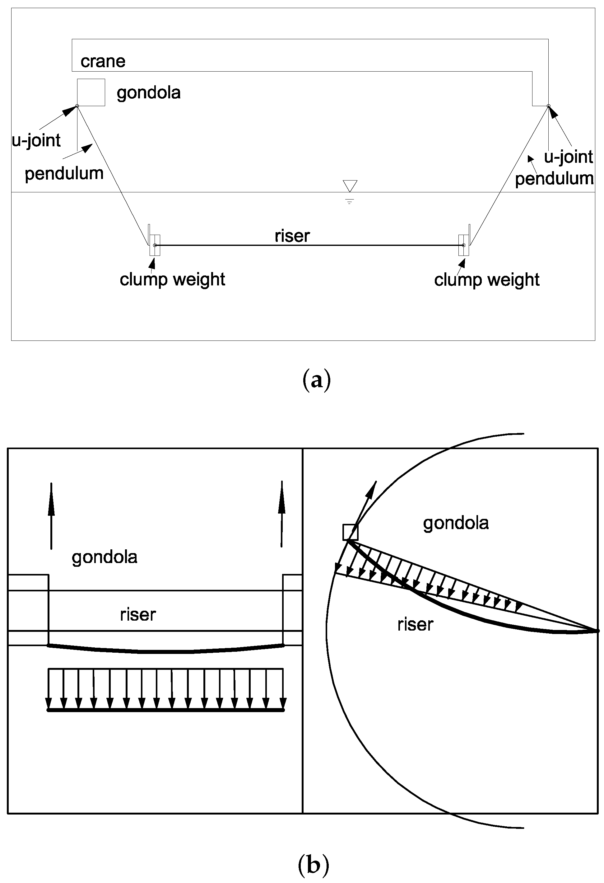
Figure 2.
Measured CF and IL fatigue damage rates (per year) for the four NDP data sets.
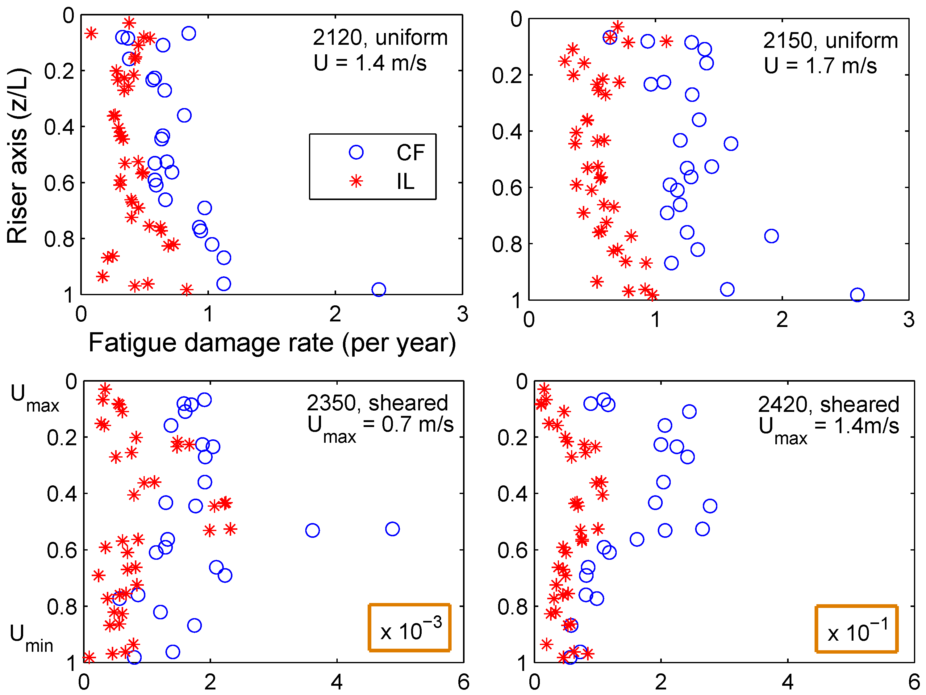
Figure 3.
The WWA procedure applied with twenty-three input sensors (sensor no. 4 is the target) for the NDP2350 (sheared current) data set: (a) PSDs of the strains measured at the twenty-three sensors; (b) summation of the strain PSDs at each frequency and identification of the selected modes; (c) strain PSD at the target sensor, reconstructed vs. measured; and (d) RMS curvatures, reconstructed vs. measured.
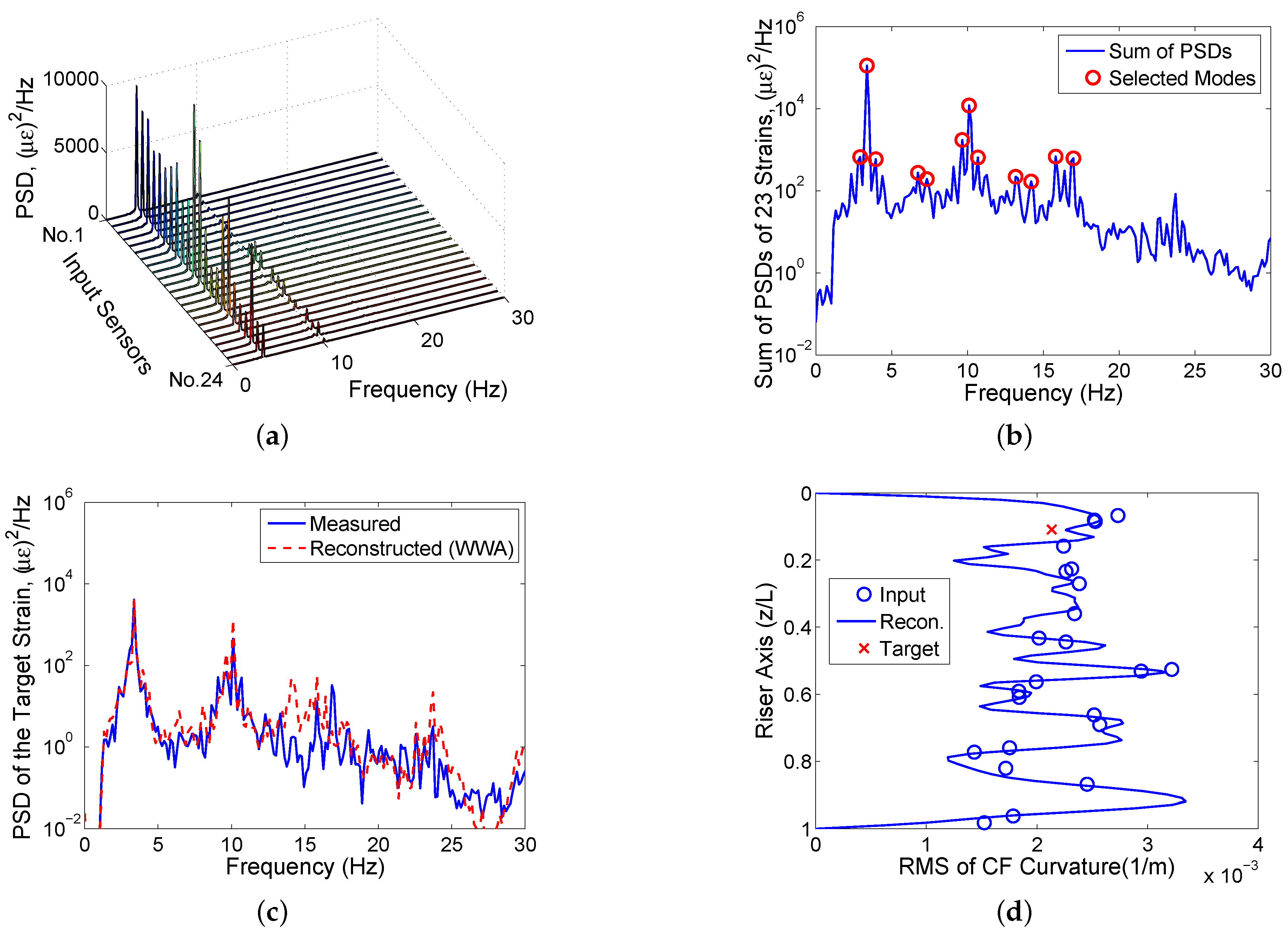
Figure 4.
The modified WWA procedure applied with twenty-three input sensors (sensor no. 4 is the target) for the NDP2350 (sheared current) data set: (a) PSDs of the strains measured at the twenty-three sensors; (b) summation of the strain PSDs at each frequency and identification of the selected modes; (c) strain PSD at the target sensor, reconstructed vs. measured; and (d) RMS curvatures, reconstructed vs. measured.
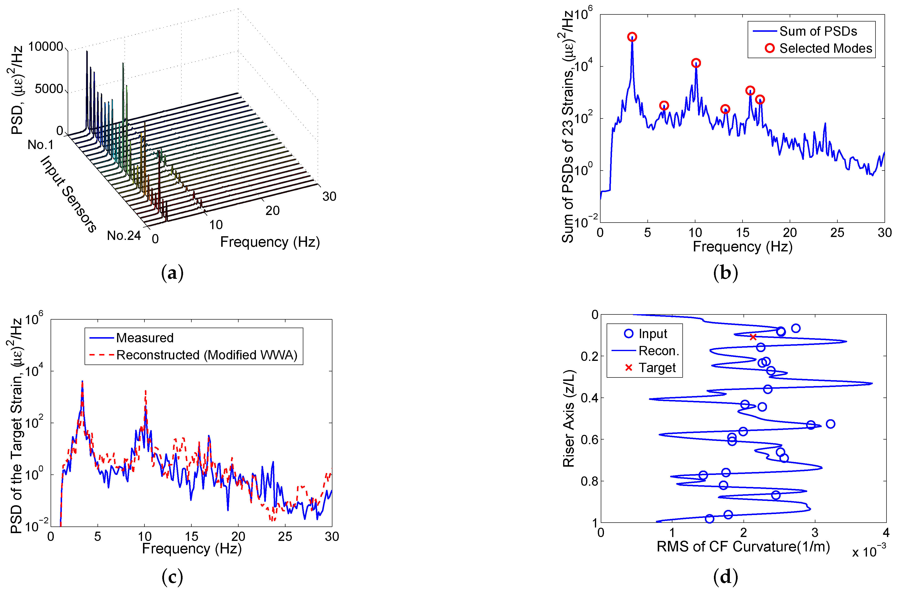
Figure 5.
The POD procedure applied with twenty-three input sensors (sensor no. 4 is the target) for the NDP2350 (sheared current) data set: (a) PSDs of the strains at the twenty-three sensors reconstructed using the first thirteen POD modes; (b) summation of the strain PSDs at each frequency using the first thirteen POD modes; (c) strain PSD at the target sensor, reconstructed using thirteen POD modes vs. measured; and (d) RMS curvatures, reconstructed using thirteen POD modes vs. measured.
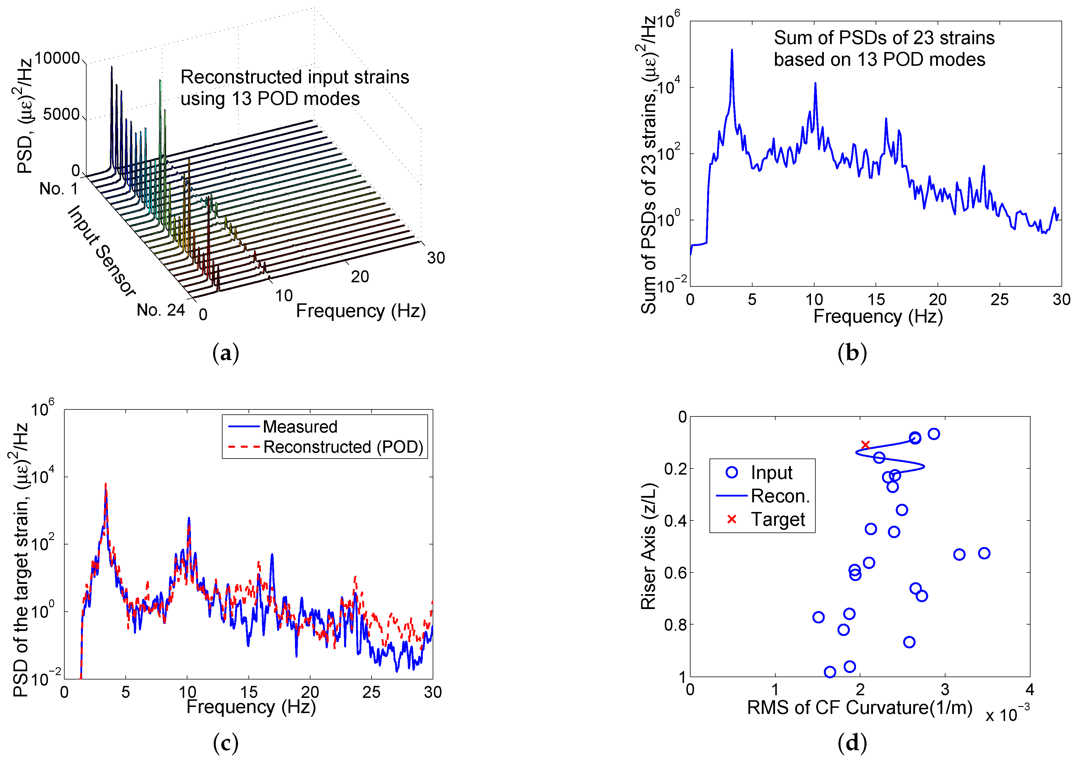
Figure 6.
The MPR procedure applied with twenty-three input sensors (sensor no. 4 is the target) for the NDP2350 (sheared current) data set: (a) PSDs of the strains measured at the twenty-three sensors; (b) summation of the strain PSDs and the frequency components that preserve 99% energy; (c) strain PSD at the target sensor, reconstructed (using modes that preserve 99% energy) vs. measured; and (d) RMS curvatures, reconstructed (using modes that preserve 99% energy) vs. measured.
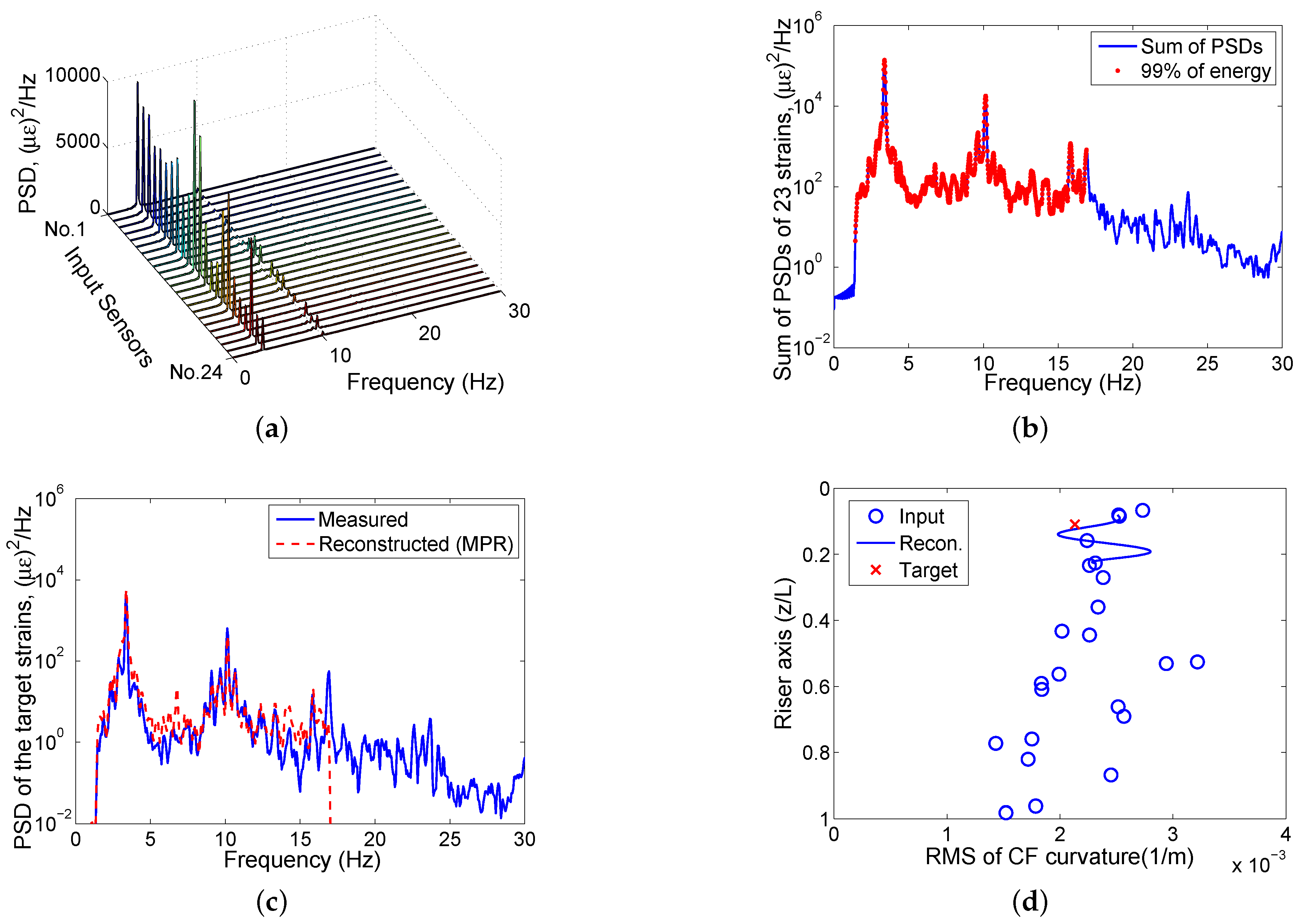
Figure 7.
The hybrid (MPR + modified WWA) procedure applied with twenty-three input sensors (sensor no. 4 is the target) for the NDP2350 (sheared current) data set: (a) PSDs of the strains measured at the twenty-three sensors; (b) summation of the strain PSDs and the frequency components that preserve 99% energy; (c) strain PSD at the target sensor, reconstructed (using modes that preserve 99% energy) versus measured; and (d) RMS curvatures, reconstructed (using modes that preserve 99% energy) vs. measured.

Figure 8.
Variability factors estimated by different empirical methods at all locations along the NDP model riser, using twenty-three stains as inputs: (a) WWA; (b) Modified WWA; (c) POD; (d) MPR; and (e) Hybrid: MPR + modified WWA.
Figure 8.
Variability factors estimated by different empirical methods at all locations along the NDP model riser, using twenty-three stains as inputs: (a) WWA; (b) Modified WWA; (c) POD; (d) MPR; and (e) Hybrid: MPR + modified WWA.
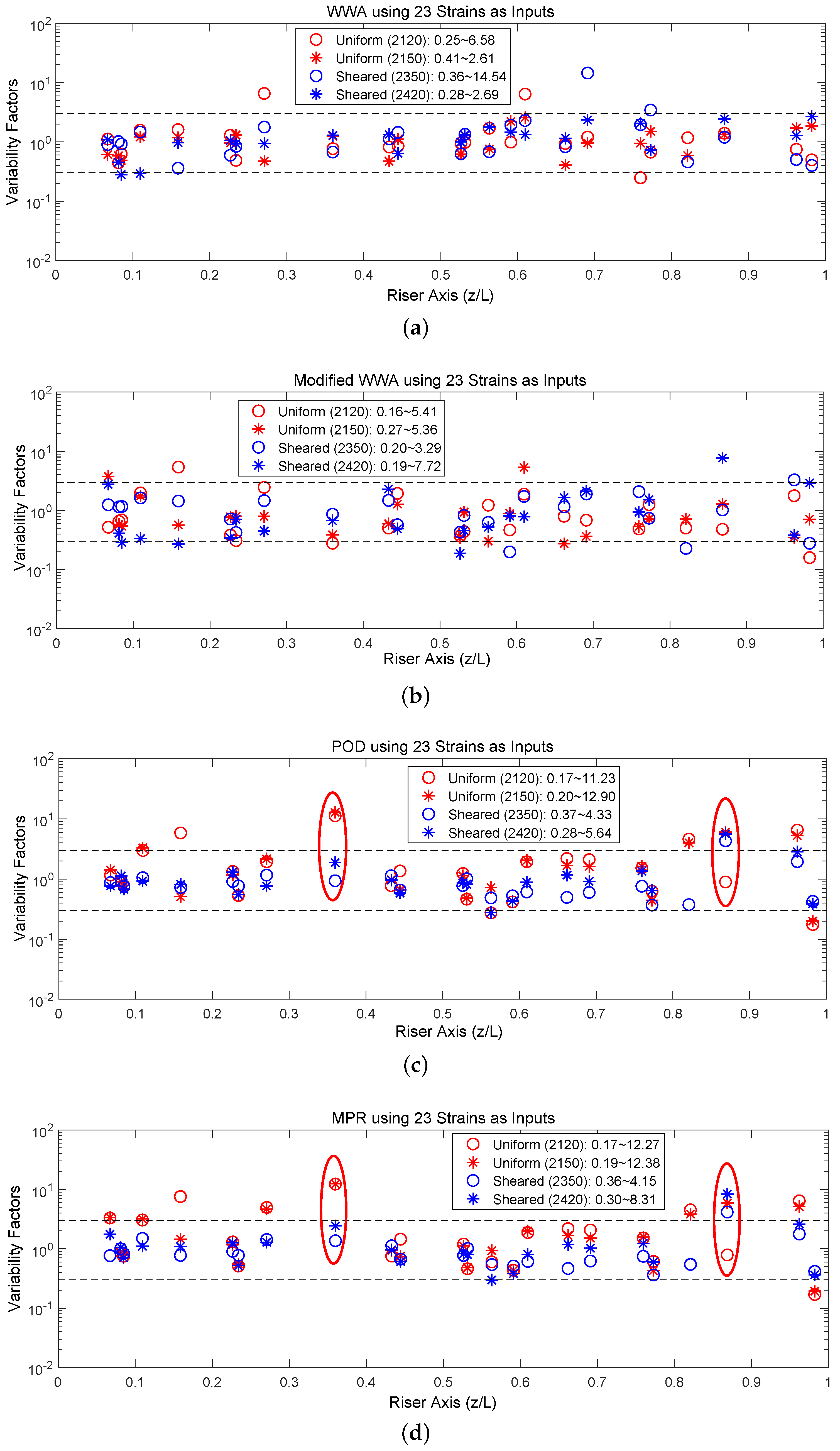
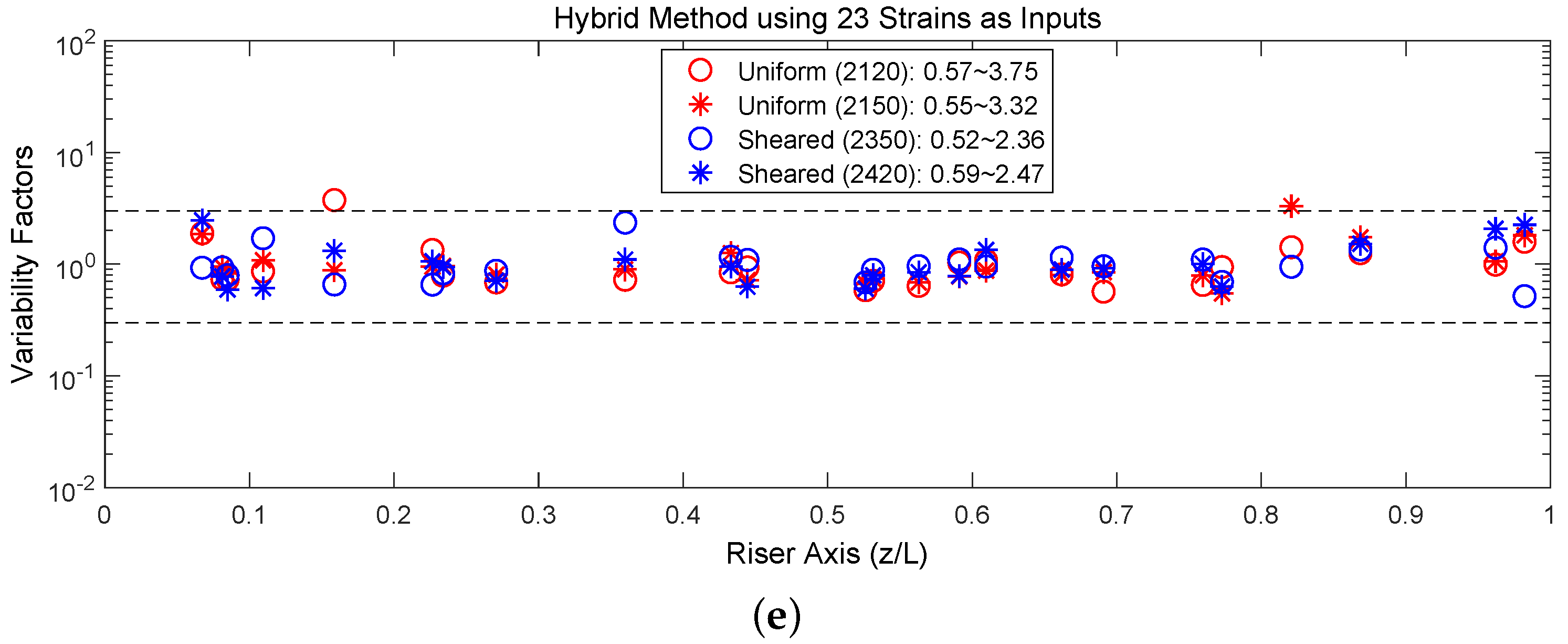
Figure 9.
Alternative parameters that might be used to evaluate the reconstructed riser response; these include the variability factor (ratio of the fatigue damage rates), the ratio of RMS values of strains, and the ratio of RMS values of displacements.
Figure 9.
Alternative parameters that might be used to evaluate the reconstructed riser response; these include the variability factor (ratio of the fatigue damage rates), the ratio of RMS values of strains, and the ratio of RMS values of displacements.
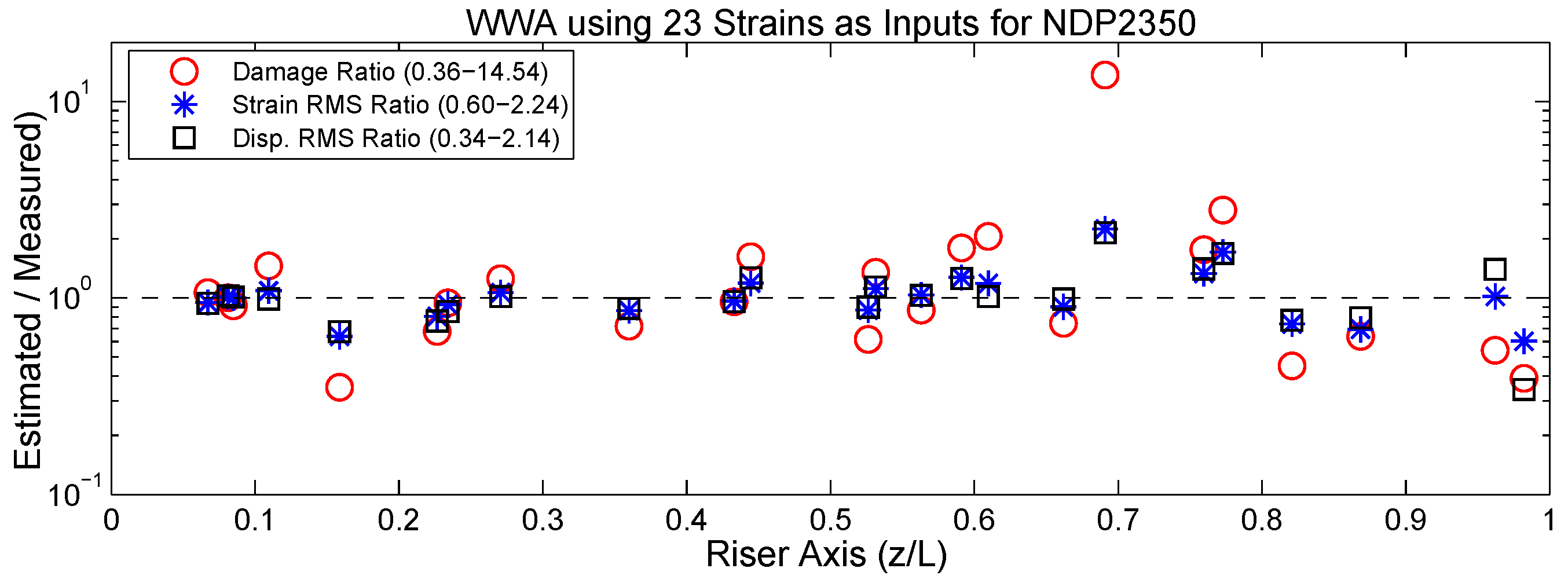
Figure 10.
Thirty-four combinations of eight input strain sensors chosen for fatigue damage analysis studies using cross-validation against measurements.
Figure 10.
Thirty-four combinations of eight input strain sensors chosen for fatigue damage analysis studies using cross-validation against measurements.
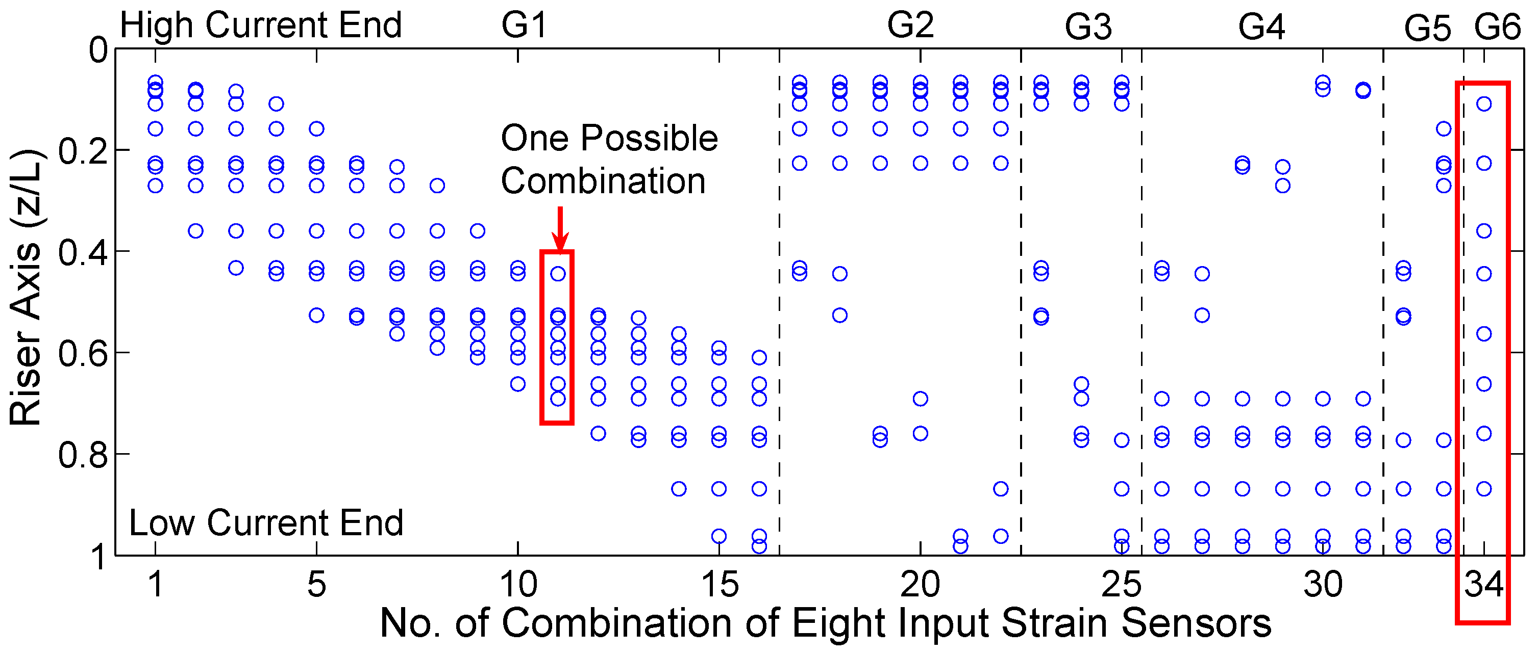
Figure 11.
Variability factors estimated by the WWA method from measurements based on thirty-four combinations involving eight strain sensors: (a) two uniform current data sets; and (b) two sheared current data sets.
Figure 11.
Variability factors estimated by the WWA method from measurements based on thirty-four combinations involving eight strain sensors: (a) two uniform current data sets; and (b) two sheared current data sets.
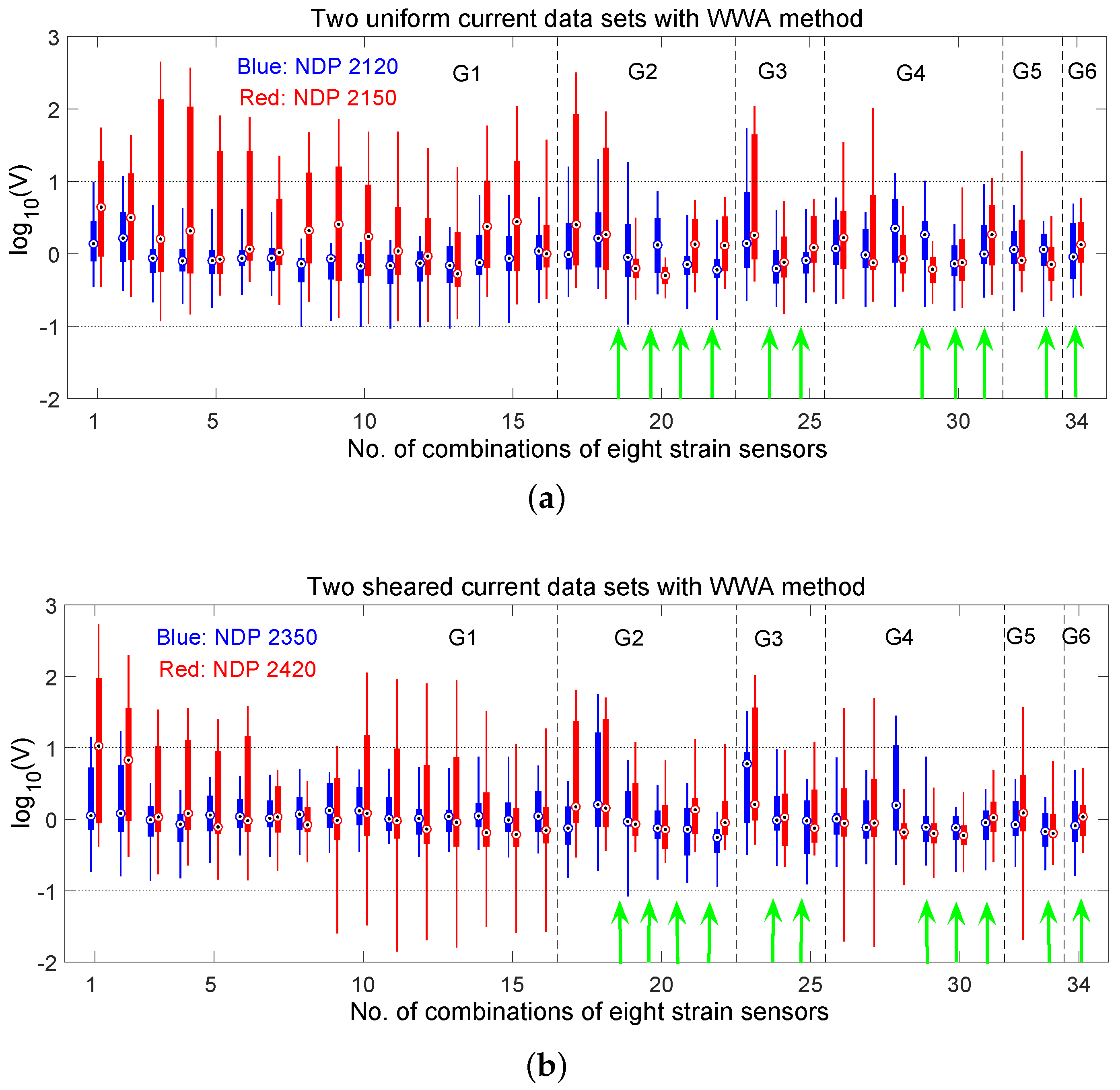
Figure 12.
Variability factors estimated by the hybrid method based on thirty-four combinations involving eight strain sensors: (a) two uniform current data sets; and (b) two sheared current data sets.
Figure 12.
Variability factors estimated by the hybrid method based on thirty-four combinations involving eight strain sensors: (a) two uniform current data sets; and (b) two sheared current data sets.


Figure 13.
Off-diagonal elements of orthogonality matrices, R, computed with assumed sinusoidal mode shapes for the NDP2350 (sheared current) data set: (a) twenty-three sensors and twelve WWA modes used (sensor no. 4 is the target); and (b) eight sensors and four WWA modes (combination no. 34).
Figure 13.
Off-diagonal elements of orthogonality matrices, R, computed with assumed sinusoidal mode shapes for the NDP2350 (sheared current) data set: (a) twenty-three sensors and twelve WWA modes used (sensor no. 4 is the target); and (b) eight sensors and four WWA modes (combination no. 34).
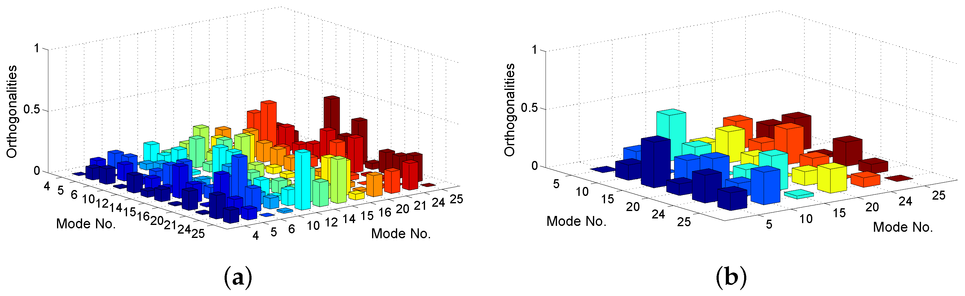

Table 1.
Physical and hydrodynamic properties of the NDP model riser.
| Length (m) | 38 |
| Outer diameter (mm) | 27 |
| Wall thickness (mm) | 3 |
| Mass of riser per unit length (kg/m) | 0.933 |
| Mass of displaced water per unit length (kg/m) | 0.576 |
| Mean effective tension (N) | 4000 to 6000 |
| Bending stiffness (N-m2) | 598.8 |
| Maximum Reynolds number | ∼70,000 |
Table 2.
The four bare riser NDP data sets.
| Event No. | Current Profile | Max. Current Speed (m/s) | Largest RMS CF-disp./D | Duration (s) |
|---|---|---|---|---|
| 2120 | Uniform | 1.4 | 0.44 | 25 |
| 2150 | Uniform | 1.7 | 0.40 | 18 |
| 2350 | Sheared | 0.7 | 0.42 | 60 |
| 2420 | Sheared | 1.4 | 0.37 | 27 |
© 2018 by the authors. Licensee MDPI, Basel, Switzerland. This article is an open access article distributed under the terms and conditions of the Creative Commons Attribution (CC BY) license (http://creativecommons.org/licenses/by/4.0/).
Share and Cite
MDPI and ACS Style
Shi, C.; Manuel, L.; Tognarelli, M. A Comparison of Empirical Procedures for Fatigue Damage Prediction in Instrumented Risers Undergoing Vortex-Induced Vibration. Appl. Sci. 2018, 8, 2085. https://doi.org/10.3390/app8112085
AMA Style
Shi C, Manuel L, Tognarelli M. A Comparison of Empirical Procedures for Fatigue Damage Prediction in Instrumented Risers Undergoing Vortex-Induced Vibration. Applied Sciences. 2018; 8(11):2085. https://doi.org/10.3390/app8112085
Chicago/Turabian StyleShi, Chen, Lance Manuel, and Michael Tognarelli. 2018. "A Comparison of Empirical Procedures for Fatigue Damage Prediction in Instrumented Risers Undergoing Vortex-Induced Vibration" Applied Sciences 8, no. 11: 2085. https://doi.org/10.3390/app8112085
Note that from the first issue of 2016, this journal uses article numbers instead of page numbers. See further details here.