UAV Motion Strategies in Uncertain Dynamic Environments: A Path Planning Method Based on Q-Learning Strategy †


1
UAV Application Engineering Department, Air Force Engineering University, Xi’an 710038, China
2
69220 Troops, People’s Liberation Army, Aksu 842000, China
*
Authors to whom correspondence should be addressed.
†
Project supported by the National Natural Science Foundation of China (Grant No. 61603411).
Appl. Sci. 2018, 8(11), 2169; https://doi.org/10.3390/app8112169
Submission received: 15 September 2018
/
Revised: 21 October 2018
/
Accepted: 31 October 2018
/
Published: 6 November 2018
(This article belongs to the Special Issue UAV Assisted Wireless Communications)
Abstract
:A solution framework for UAV motion strategies in uncertain dynamic environments is constructed in this paper. Considering that the motion states of UAV might be influenced by some dynamic uncertainties, such as control strategies, flight environments, and any other bursting-out threats, we model the uncertain factors that might cause such influences to the path planning of the UAV, unified as an unobservable part of the system and take the acceleration together with the bank angle of the UAV as a control variable. Meanwhile, the cost function is chosen based on the tracking error, then the control instructions and flight path for UAV can be achieved. Then, the cost function can be optimized through Q-learning, and the best UAV action sequence for conflict avoidance under the moving threat environment can be obtained. According to Bellman’s optimization principle, the optimal action strategies can be obtained from the current confidence level. The method in this paper is more in line with the actual UAV path planning, since the generation of the path planning strategy at each moment takes into account the influence of the UAV control strategy on its motion at the next moment. The simulation results show that all the planning paths that are created according to the solution framework proposed in this paper have a very high tracking accuracy, and this method has a much shorter processing time as well as a shorter path it can create.
1. Introduction
It is not easy for an unmanned aerial vehicle (UAV) to fly autonomously in uncertain, dynamic environments; this concerns the safety of the UAV itself as well as that of the air traffic controllers. In recent years, the safety of UAVs has become a focus in the aviation realm, as unmanned aerial vehicles are used for more and more applications [1]. Related accident survey and analysis show that, because of equipment breakdown and ground operator error, unavoidable crashes make up the majority of all aviation accidents. If this kind of unavoidable aviation accident cannot be handled well, it will greatly restrict the development of UAVs [2]. How to handle this problem is still a challenge.
Path planning for UAV is a key technique in UAV navigation and automation [3,4]. A path planning problem for UAV is defined according to the mission requirements and constraints, and then establishes a secure, feasible, and optimal flight path from the start to the target [5]. The dynamic path planning for UAV faces extreme challenges not only because there are many complicated and uncertain factors in its application environment, but also because there are strong uncertainties, magnitude fuzzy, and coupling among these interaction factors and constraints, together with the unique mission and control mode to UAV [6]. In order to solve the problem of flight decision of UAV in uncertain dynamic environments using a path planning method, the following studies should be included.
- Learning and cognition in an unstructured environment. In general, learning and cognition are key behaviors of human beings. However, in unstructured environment, there is no established information for the UAV to use directly. If it wonders where to go, it must explore the environment like a person. As a result, learning and cognition become very important for UAVs to fly in such an unstructured environment.
- Real-time planning and re-planning. In fact, a preplanned flight path will not meet the demands of an actual flight for a UAV, because there would not always exist a path suitable for the UAV to fly in an unstructured environment. It must re-plan a flightworthy path according to the actual circumstances. Real-time planning and re-planning forma complex problem that involves meeting the physical constraints of the UAVs, constraints from the operating environment, constraints from the threat or no-fly zones, and other operational requirements.
- Multi-UAVs’ collaborative planning and control. Multi-UAV collaborations have become a vital platform in the military field, and will also be the cutting-edge technologies in the future. Enabling the multi-UAV effective autonomous cooperative wide area target search ability is the key to carrying out the task chain of search, attack, and evaluation, so research on such a problem has a very important military application value. To obtain an effective autonomous cooperative search, the UAV platform must be equipped with the ability of autonomous decision-making, which is dealing with these basic problems: decision-making structure, information model, decision-making method, and also dealing with two extended problems, delayed information compensating and system scale control. In the future, the above problems should be well studied and a UAV autonomous cooperative wide area target search mechanism should be established as well.
- Automatic generation and calculation of flight strategy. We develop the UAV and hope it can fly autonomously without human control. As a result, unlike remote control systems in which the sensors present information in a form that is as operator-friendly as possible, in a UAV, a system platform that performs the autonomous mission usually possesses an onboard navigation system instead of sensors of various physical nature. So, the measurement results should be converted into input signals of the control system, which requires other approaches. At the same time, in an autonomous flight, the observing system should be able to search for characteristic objects in the observed landscape and give the control system their coordinates and estimate the distances between them [7]. So, it is very important to study how to produce a decision/control that can be executed directly by the onboard control system.
As far as a path planning application is concerned, not only should the direct impact of various constraints on the UAV movement be considered, but also the real-time control instructions should be calculated according to feedback information that might have an effect on the current motion state of the UAV. Furthermore, the planning system sometimes could not sense the current exact state completely because of the threats and the unknown environment as well as the error and imperfection owing to the precision of the sensors and the current position, velocity, acceleration, and poses of the UAV to be estimated according to the action strategy it adopted. As a result, not only the uncertainty of the actions but also the uncertainty of the states should be considered in the actual path planning for UAV; this happens to accord with the partially observable problem, and belongs to the category of partially observable Markov decision process theoretical research. Consequently, a dynamic path planning solution framework for UAV constructed based on Q-learning theory is suitable, and in this solution framework, we consider the effects of the uncertainty environment along with the optimal control strategy and the dynamics of the UAV together during the path planning. This is in line with the application of UAV path planning, and further improves the navigation accuracy.
The rest of this paper is organized as follows. First, some related work is introduced in Section 2. Then, Q-learning theory and a path planning model based on Q-learning strategy are described in Section 3; meanwhile, a path planning solving framework for UAV based on Q-learning strategy is constructed. In this framework, the uncertainty owning to the environment is considered as well as the effect of the movement changing after the UAV adopted the planned control strategies. Following that, the state transition of the path planning for UAV is described, the cost function is defined, and strategy creation for UAV path planning based on Q-learning theory is elaborated on in Section 4. The findings of the method proposed in this paper are illustrated with simulations and analysis in Section 5. Finally, Section 6 concludes this paper.
2. Related Work
There are many studies on dynamic path planning. The Voronoi map algorithm [8] is the most famous one. Although the Voronoi map algorithm can solve this kind of complicated problem and find the shortest planning path, the computational complexity increases with the complexity of the problem, and it does not handle sudden threats well. A potential field function was introduced by Khabit [9] to describe the geometrical structure of space and depict the motion planning problem accordingly. Although the artificial potential field method has a small amount of calculation and a fast planning speed, there exists a local minimum where the attraction equals the repulsion. Consequently, the path may become a trap area during planning and vibrate in a narrow channel easily. Chen’s method [10] mends this bug using a tangent-plus-Lyapunov vector field in the dynamic path planning for UAV, conquering the problem of the local minimum; at the same time, this method does not take the planning influence into account, which was caused by the change incontrol strategy.
In recent years, swarm intelligent optimization algorithms including particle swarm optimization [11], ant colony optimization [12], and artificial bee colony algorithm [13] have emerged for path planning. These algorithms generally adopt a parallel mechanism to deal with the calculations. Although they are more suitable for solving complex continuous optimization problems, they are not quite fit for asituation in which there are multiple objective constraints and their interaction/influence. In addition, these algorithms are prone to a local minimum, or the calculation complexity increases exponentially with the size of the problem, even to the extent of leading to a combination explosion. Artificial intelligent information theory methods for motion planning problems are specifically summarized in the literature [14]. Notwithstanding, the genetic algorithm [15], evolutionary algorithm [16,17], and artificial neural network algorithm [18] can handle some specific path planning applications, yet necessary compensation for the whole planning system is seldom included in these artificial intelligent algorithms because the UAV’s motion state is changed by the control strategy or environmental changes are notconsidered.
In the last two or three years, many new autonomous decision-making as well as path planning methods have emerged. Lee and Bang [19] improved the particle filter(PF)-based terrain-aided navigation(TAN) method, which has been commonly used to obtain stable real-time navigation solutions in cases where the UAV operates at a high altitude. They designed a Rao‒Blackwellized PF (RBPF)-based TAN, used long short-term memory (LSTM) networks to endure flat and repetitive terrains, and trained the noise covariances and measurement model of RBPF, and they confirmed that the proposed algorithm can enable more precise navigation performance than conventional RBPF-based TAN through simulations. With the development of deep learning theory, some machine learning methods have emerged one after another in UAV flight control and flight decision-making. Li [20] developed an off-policy reinforcement learning (RL) algorithm to solve optimal synchronization of multiagent systems, which is a model-free approach in that it solves the optimal synchronization problem without havingany knowledge of the agent dynamics, and it can synchronize all agents to the leader. Zhang [21] studied an optimal consensus tracking problem of heterogeneous linear multiagent systems, and found a Nashequilibrium solution by solving associated coupled Hamilton‒Jacobi equations. The optimal cooperative control can be obtained by the input‒output (I/O) Q-learning algorithm, and the numerical example proved that the algorithm does not rely on the model of multiagent systems. These two methods could be used to handle the multi-UAVs collaborative planning and control problem.
Recent research has also focused on decision-making, formation control, and 3D/4D path planning. For example, Zhao [22] proposed a brain-inspired decision-making spiking neural network (BDM-SNN) and applied it to decision-making tasks on UAVs. Park [23] addressed the analysis and deployment of the network infrastructure based on multiple Unmanned Air Vehicles in his new research. He modeled the generic dynamics of the network infrastructure, derived the network throughput of the infrastructure, and proposed a novel formation control algorithm that determines the location of the UAVs to maximize the efficiency of the network. Halil’s [24] comparison of 3D versus 4D path planning for UAVs used empirical data and showed that the 4D approach is superior to the 3D approach, especially in complex, dynamic environments, through a series of simulations.
3. UAV Path Planning Model Based on Q-Learning Strategy
3.1. Q-Learning Theory
Q-learning [25] is a reinforcement learning [26] strategy adoption rule, whereby agents learn an optimal strategy, maximizing their expected reward in the repeated game. That is to say, Q-learning describes an agent that uses unsupervised training to learn about an unknown environment. In general, we call where an agent is a “state.” The agent’s movement from one position to another is an “action.” As shown in Figure 1, a “state” is depicted as a node, while “action” is represented by the arrows.
The matrix R can be viewed as a reward table as shown in Figure 2. Suppose the agent is in state 2. From state 2, the agent can go to state 3 because state 2 is connected to 3. From state 2, however, the agent cannot directly go to state 1 because there is no direct arrow connecting state 1 and 2. From state 3, it can go either to state 1 or 4 or back to 2 (look at all the arrows around state 3). If the agent is in state 4, then the three possible actions are to go to state 0, 5 or 3. If the agent is in state 1, it can go either to state 5 or 3. From state 0, it can only go back to state 4. We can put the state diagram and the instant reward values into the following reward table, “matrix R.” In order to make the agent more intelligent, we add a similar matrix, “Q,” to the agent as a brain, representing the memory of what the agent has learned through experience. The rows of matrix Q represent the current state of the agent, and the columns represent the possible actions leading to the next state (the links between the nodes).
At first, the agent starts out not knowing anything, so the matrix Q is initialized to zero. For the simplicity of explanation, we assume the number of states is known (six). If we did not know how many states were involved, the matrix Q could start out with only one element. It is a simple task to add more columns and rows in matrix Q if a new state is found. The transition rule of Q-learning is a very simple formula:
So far, according to the above formula, a value assigned to a specific element of matrix Q is equal to the sum of the corresponding value in matrix R and the learning parameter , multiplied by the maximum value of Q for all possible actions in the next state. The virtual agent will learn through experience, without a teacher (this is called unsupervised learning). The agent will explore from state to state until it reaches the goal. We will call each exploration an episode. Each episode consists of the agent moving from the initial state to the goal state. Each time the agent arrives at the goal state, the program goes to the next episode.
Owing to the unstructured environment, the state of the environment and the actions taken by the UAV are not fully observable. So, in this problem, we assumed that the environment constituted a partially observable Markov decision process (POMDP) [27], which is a controlled dynamical process in discrete time useful for modeling resource control problems. Accordingly, UAV path planning is a highly complex problem, and can be described as a dynamical control process with a hidden Markov process. The following subsection bridges the gap between them.
3.2. Specification of the Motion Strategies Problems
In general, a motion strategies problem structure appears as in Figure 3. It can be defined in a Q-learning problem by a 5-tuple like , where denotes an observable hidden Markov decision model of the system, is the state set, and is the action set of the system. State transition function denotes the probability that the system state will transfer from to when it takes action . Observation set denotes a set that the system can be measured. Observation function denotes that the probability distribution of the system state can be fully observed and that the system state is transferring from to when it takes action .
3.3. The Solution Framework for UAV Path Planning Based on Q-Learning
Suppose that the state of the UAV motion is partially observed, and that there are some hidden states that can be observed in the system that satisfied the Markov attribute. Then this problem can be transformed into a Q-learning problem and described as follows.
Let be the system state of the UAV path planning system at time , where denotes the states of the sensors; the position, velocity, acceleration, and detection information of the flight environment are included. denotes the standard path for UAV, including the longitude, latitude, and altitude information of the path points. represents the state of the path planning, and is a standard Kalman filter, where and are the posterior mean vector and covariance matrix, respectively.
If the acceleration and bank angle of the UAV are chosen as the controlled variables, then the action at time can be represented as , where and denote the acceleration and the bank angle at time of the UAV, respectively.
The effect of the action that the UAV adopts should be considered in the state transition of the system. Let and denote the position of the standard path point and the current position of the UAV, respectively; then the observation function of the system can be represented as follows:
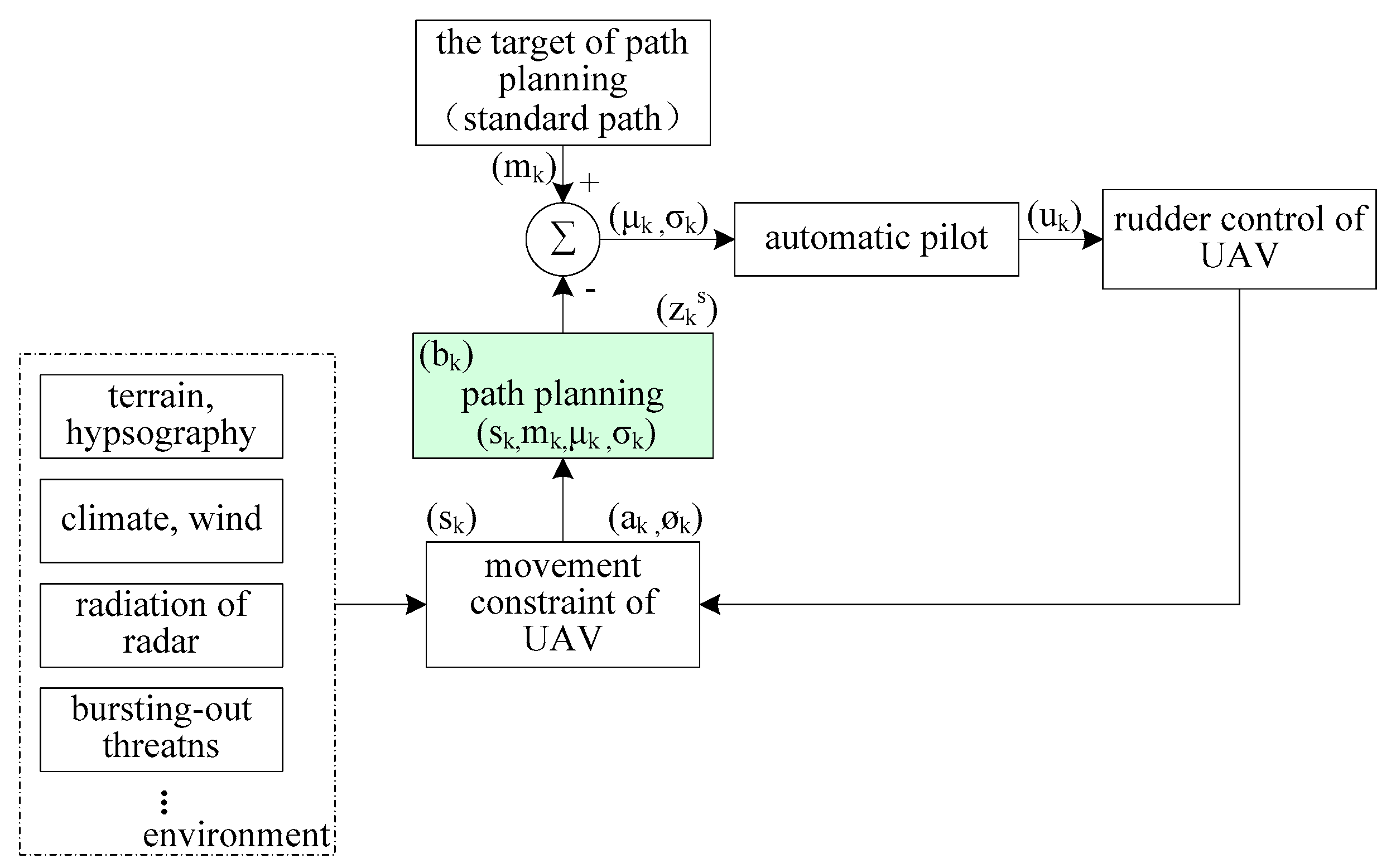
where denotes the observation model and is the random observation error. The distribution of depends on the position of the UAV and the position of the standard path point , and the system frame of the UAV path planning based on POMDP is shown in Figure 4.
4. Strategy Creation for UAV Path Planning Based on Q-Learning
For the dynamic path planning problem for UAV, the planning strategy creation should include the effect that the flight control suffered from the random environment as well as the system dynamic attribute to the control affect of the UAV. If we take the posterior distribution about the hidden state of the system calculated according to the Bayes rule as the belief state, then the optimal control strategy of the UAV dynamic path planning can be given according to Q-learning theory following Bellman’s optimization principle.
4.1. The System State Transition of UAV Path Planning
The state transition of the system depends on the action strategies for the UAV under the control; the motion of the UAV must be considered accordingly during the problem solving process. Let us suppose that all the sensors are fixed up to the airframe and there are no distortions of them; then, the state updating of the sensors can be regarded as the status update after the UAV takes the action strategy.
If the state of UAV at time is given by , where represents the position coordinates, denotes the instant velocity, and is the heading angle of the UAV at time , then, the state updating of the UAV can be described as
where is a mapping function that constructs the correlation between the control variables and the movement of the UAV, and can be collected by a group of simple equations that govern the UAV kinematics motion. For the sake of establishing the relationships between the control actions and the movements of the UAV, we choose the control actions as follows:
The control action can be deduced from the kinematics motion equations of the UAV, and the speed and the heading angle of the UAV are updated according to the flight mechanics theories as follows:
Specifically,
where and denote the minimum and maximum limits on the speed of the UAV, respectively; is the acceleration of gravity; and is the length of the planning time step.
The position coordinates of the UAV are updated as follows:
4.2. Cost Function
The cost function is defined by the solution of mean square error between the current path and the standard path, that is,
where is an independent and identically distributed random noise signal superimposed on the standard path information, and its value lies in the precise measurement of the sensors on board and the effect of communication noise.
4.3. The Optimal Strategy for UAV Path Planning Based on Q-Learning
Generally speaking, the target of UAV path planning problem is a minimum mean square cumulative error between the current solving path and the standard path over a given time sequence , and the expected cumulative error on the time sequence can be described as
The action selection of the UAV at time depends on the observation measurements of all the former time. If there is an optimal action that would lead the UAV to the expected path at time , then there is an optimal action sequence relying on the feedback of the belief state. Therefore, the cost function can be given as below:
where,
Belief state is the posterior probability distribution of hidden states of the UAV path planning system at time , that is,
where , , , and is the posterior probability distribution of the standard path information measured by the onboard sensors of the UAV.
According to Bellman’s optimal principle [28], the optimal cost function value under the current given belief state can be written as
where is the random value of the belief state at the next time step, is the optimal cumulative cost over the time sequence , and denotes the conditional expectation under the given current belief state at time and after the UAV taking the action .
Accordingly, the optimal strategy at time can be given as below:
Consequently, the optimal control strategy of arriving at the target path at time is
However, in practice the second term in the optimal control strategy (the above formula) is hard to obtain exactly; therefore, this problem needs to be transformed as follows in order to find the optimal answer.
Suppose the UAV always takes the optimal flight control strategy at every flying path point starting from time ; if the optimal action sequence corresponds to the optimal cumulative cost function over the time sequence is , the covariance matrix sequence among the planned optimal path points is .
Because the measurement of the system is related to the standard path information and the movement state of the UAV, the measurement error comes from two aspects, the estimation of the standard path and the estimation of the movement state of the UAV itself. According to the observation model, as Equation (1) shows, if the standard path information is fully observed, there is a partially observable hidden state in the current movement of the UAV. If we suppose that the observation noise of the sensors obeys zero-mean Gauss distribution, then the measurement error distribution of the system at time is
Accordingly, the belief level of the system observation at present is
where
The observation model of the standard path according to the measurements from the onboard sensors of UAV is
where is an identity matrix; since the standard path is determined in advance, the dynamic of the standard path can be seen as the direct measurement according to the onboard sensors relative to the UAV, that is to say, Equation (20) can be regarded as a dynamic model of the standard path superimposing the onboard sensors’ measurement error.
Then, according to matrix theory and stochastic process theory, we have
Combining with Equation (2), it can be seen in Equation (19) that the covariance matrix of the system at time depends on the measurements at that time. Since these observations cannot be measured exactly, the position of the UAV at time can only be approximated by the measurements of the standard path at the exact time, and it needs to be adjusted according to the line of sight between the sensors and the standard path. Consequently, the minimum mean square covariance of the current planning path and the standard path, that is to say, the cost function of the path planning system, can be written as below:
Accordingly,
Consequently, the corresponding optimal control strategy of the UAV path planning based on Q-learning can be obtained with the minimum value of Equation (24) winning.
To handle the hidden state uncertainty of the UAV path planning problem, we suppose there is distance uncertainty and angle uncertainty in the observation covariance distribution of the system, and accordingly, if the position coordinates of the standard path at time are , then the standard deviation between the planning path and the standard path at time is denoted below:
If the intersection angle among the standard path point to the centroid of the UAV and the axes of the sensor is , then the process noise covariance matrix can be calculated as below:
where
Obviously, the eigenvalues of the matrix are .
5. Simulation and Analysis
The simulations are executed to validate the effectiveness of the proposed method on a lab computer, with an Intel® Core™ i3-2120 3.3 GHz CPU with 2 GHz EMS memory, Windows XP as the operating system, and Matlab R2012a involved in the verification as the development environment. To be exact, let us suppose that the original position of the UAV is at , the original speed is , and , . The initial distance error of the inertial system is , its horizontal velocity error is , and its angle error is ; furthermore, let , , that is to say, there is 10% distance uncertainty and % angle uncertainty in the error distribution of the system. The receding horizon control technique is adopted in order to get an optimal control sequence during the planning process. Specific speaking, six time steps corresponding to state evolutions of the system are planned at every discrete time simultaneously, but only the first control signal in the planned optimal control sequence of them is taken to act on the system, and the other five are abandoned. This process is repeated ceaselessly during the simulations; consequently, here , and the whole planning time .
The flight path of the UAV is shown in Figure 5; from the simulation results we can see that the actual path based on the Q-learning method in this paper is almost identical to the standard path.
Combined with the inertial navigation system, electronic compass, altitude indicator, and laser range finder fitted in the UAV, the combined fusion system ascertains the actual current position and state of the UAV itself according to the planning path that was obtained after the automatic pilot system manipulated the rudder plane at every discrete time. Figure 6 shows the estimated error between the planning path based on the method proposed in this paper and the standard path.
The errors in the position and the flight attitude are both greatly suppressed during the simulations by using the method proposed in this paper. From the simulation results, we can see that the estimated error of the flight altitude is less than , the estimated error of the angle is less than , and the estimated error of the velocity in the horizontal direction is less than .
Assuming that the threat is moving in a uniform straight line, the trajectory for the UAV to avoid the motion threat at different angles is given in Figure 7, where the red track is the trajectory of the motion threat and the black track is the trajectory of the UAV. The black dots in the threat trajectory are the waypoints predicted by Q-learning that may cause the conflict, and the black arrow indicates the direction of motion of the UAV and the threat, respectively. From Figure 7 we can see that, Although there is an intersection between the black and red trajectories, the intersection is where the threat and the UAV arrive at different times, so the two trajectories do not cause a risk of collision.
Figure 7 examines six moving threat avoidance situations at the same speed and in different directions in our method, and we list the results in Table 1. From the statistics in Table 1, it can be seen that the minimum relative distance planned by the method in this paper can achieve the minimum flight safety distance specified in the general rules of flight safety.
The simulation results of UAV avoidance under the moving threat are given in Figure 8. In the figure, the red triangle represents the moving threat, and the black triangle represents the UAV. The numbers on each triangle represent the position of the UAV and the threat at that moment. From the simulation, it can be seen that the “2” moment is the closest moment when the UAV might encounter with the moving threat, and they are likely to collide with each other if there is not any evasive action taken by the UAV.
The method proposed in this paper works like this:
When any movement conflicts within the preplanned flight path aredetected, the detection system of the UAV would immediately turn to estimate the moving threat specifically, and determine where the conflicts might occur; then, a safe flight path is estimated in advance that would not cause flight conflicts, so it can continue to fly according to the estimated flight path. According to the measurement from its own sensors and the estimated flight path and real-time altitude, the UAV modifies its flight state constantly so as to achieve the aim of conflict avoidance. This is exactly what is shown in Figure 8. The UAV has re-planned the new conflict-avoiding path before the “2” moment.
Furthermore, our method was compared with Kalman fusion, which is a standard test to track apreplanned path. Figure 9 is are sult of the comparison at the same path point. Owing to the error accumulation of the inertial navigation system, drift was produced during the simulation, but our method performs better because the control strategy at every next time step is considered in creating the path planning strategy for the exact current time step.
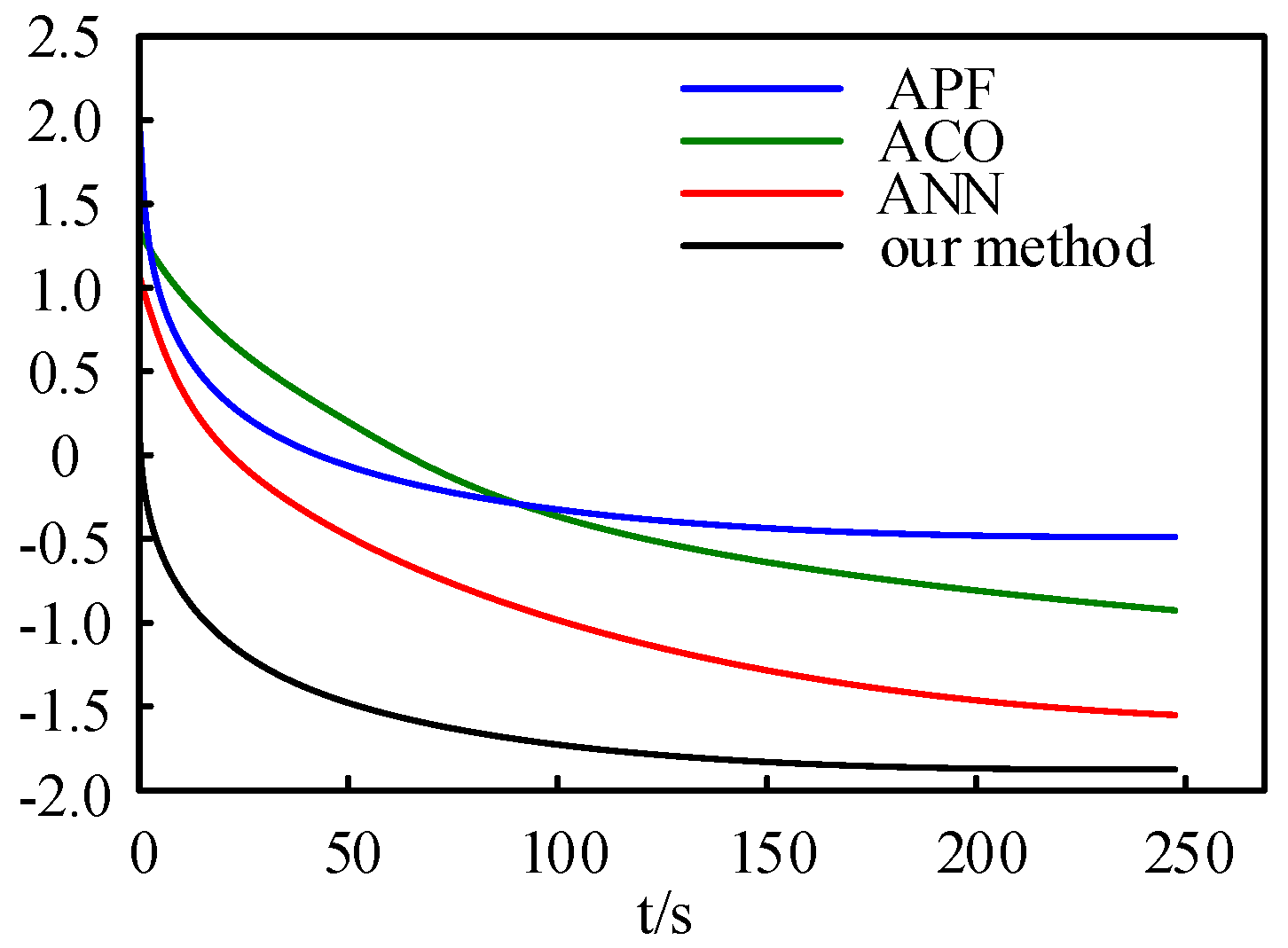
In order to verify the performance of the proposed method, we compared it with the artificial potential field (APF) [29], ant colony optimization (ACO) [30], and artificial neural network (ANN) [31], which are very popular in UAV path planning applications. Figure 10 shows the error covariance changes over time of these methods. To get a better idea of the changes, the traces of the covariance matrices were represented in a log-value coordinate form. It can be seen that the method proposed in this paper outperforms the other three.
To make a quantified comparison, Table 2 describes the corresponding quantified results of these methods. The processing time is computed by the internal counter of the simulation PC. As can be seen in the table, the APF method can create the shortest path but needs the longest processing time. In addition, owing to the iterative process during the planning, the ACO and ANN methods require more time. It can be seen from Table 1 that the method proposed in this paper can program a shorter path compared with the ACO and the ANN method. Furthermore, what is important is that this method has an extraordinarily shorter processing time.
6. Conclusions
In this paper, a dynamic path planning solution framework for UAV is proposed based on the Q-learning strategy. The effect of the uncertainty factors of the environment, as well as the feedback effect on path planning for UAV owing to the change in motion state caused by the manipulation of the automatic pilot system, is considered during the model’s construction. In the process of calculation and solution, the posterior probability distribution of the hidden state is introduced due to the existence of an incomplete observation state, and the optimal control strategy of UAV path planning can be found according to the posterior distribution of the belief state. This operating and solving process is more consistent with the actual path planning problems for UAV, by which a more accurate planning path can be found, and the simulation results show the performance and validity of this method for UAV path planning.
Author Contributions
This work presented here was completed through the collaboration of all authors. J.-h.C. proposed the idea, designed the method, and wrote the paper. R.-x.W. guided the full paper. Z.-c.L. provided writing-review. K.Z. performed partial simulation and edit.
Funding
This work was partially supported by the National Natural Science Foundation of China (Grant Number 61603411).
Conflicts of Interest
The authors declare no conflict of interest.
References
- Petritoli, E.; Leccese, F.; Ciani, L. Reliability degradation, preventive and corrective maintenance of UAV systems. In Proceedings of the 2018 5th IEEE International Workshop on Metrology for aeroSpace (MetroAeroSpace), Rome, Italy, 20–22 June 2018; pp. 430–434. [Google Scholar]
- Kanellakis, C.; Nikolakopoulos, G. Survey on computer vision for UAVs: Current developments and trends. J. Intell. Robot. Syst. 2017, 87, 141–168. [Google Scholar] [CrossRef]
- Kim, Y.; Gu, D.W.; Postlethwaite, I. Real-time path planning with limited information for autonomous unmanned air vehicles. Automatica 2008, 44, 696–712. [Google Scholar] [CrossRef]
- Bottasso, C.L.; Leonello, D.; Savini, B. Path planning for autonomous vehicles by trajectory smoothing using motion primitives. IEEE Trans. Control Syst. Technol. 2008, 16, 1152–1168. [Google Scholar] [CrossRef]
- Pachter, M.; Chandler, P.R. Challenges of autonomous control. IEEE Control Syst. Mag. 1998, 18, 92–97. [Google Scholar]
- Sun, X.J.; Wang, G.F.; Fan, Y.S.; Mu, D.; Qiu, B. An automatic navigation system for unmannedsurface vehicles in realistic sea environments. Appl. Sci. 2018, 8. [Google Scholar] [CrossRef]
- Ivan, K.; Elena, K.; Alexander, M.; Boris, M.; Alexey, P.; Denis, S.; Karen, S. Co-optimization of communication and sensing for multiple unmanned aerial vehicles in cooperative target tracking. Appl. Sci. 2018, 8, 899. [Google Scholar] [CrossRef]
- Lee, D.T.; Robert, L.; Drysdale, R. Generalization of Voronoi diagrams in the plane. SIAM J. Comput. 1981, 10, 73–87. [Google Scholar] [CrossRef]
- Khabit, O. Real-time obstacle avoidance for manipulators and mobile robots. Int. J. Robot. Res. 1986, 5, 90–98. [Google Scholar]
- Chen, H.D.; Chang, K.C.; Agate, C.S. UAV path planning with tangent-plus-Lyapunov vector field guidance and obstacle avoidance. IEEE Trans. Aerosp. Electr. Syst. 2013, 49, 840–856. [Google Scholar] [CrossRef]
- Fu, Y.G.; Ding, M.Y.; Zhou, C.P. Route planning for unmanned aerial vehicle (UAV) on the sea using hybrid differential evolution and quantum-behaved particle swarm optimization. IEEE Trans. Syst. Man Cyber.-Syst. 2013, 43, 1451–1465. [Google Scholar] [CrossRef]
- Cekmez, U.; Ozsiginan, M.; Sahingoz, O.K. A UAV path planning with parallel ACO algorithm on CUDA platform. In Proceedings of the International Conference on Unmanned Aircraft Systems (ICUAS), Orlando, FL, USA, 28–31 May 2014; pp. 347–354. [Google Scholar]
- Xu, C.; Duan, H.; Liu, F. Chaotic artificial bee colony approach to uninhabited combat air vehicle (UCAV) path planning. Aerosp. Sci. Technol. 2010, 14, 535–541. [Google Scholar] [CrossRef]
- LaValle, S.M. Planning Algorithms; Cambridge University Press: Cambridge, UK, 2006. [Google Scholar]
- Ozgur, K.S. Generation of bezier curve-based flyable trajectories for multi-UAV systems with parallel genetic algorithm. J. Intell. Robot. Syst. 2014, 74, 499–511. [Google Scholar]
- Nikolos, I.K. Evolutionary algorithm based offline/online path planner for UAV navigation. IEEE Trans. Syst. Man Cyber. B 2003, 33, 898–912. [Google Scholar] [CrossRef] [PubMed] [Green Version]
- Rahul, K. Multi-robot path planning using co-evolutionary genetic programming. Expert Syst. Appl. 2012, 39, 3817–3831. [Google Scholar]
- Saleha, R.; Sajjad, H. Path planning in robocup soccer simulation 3D using evolutionary artificial neural network. Lect. Notes Comput. Sci. 2013, 7929, 351–359. [Google Scholar]
- Lee, J.; Bang, H. A robust terrain aided navigation using the Rao-Blackwellized particle filter trained by long short-term memory networks. Sensors 2018, 18, 2886. [Google Scholar] [CrossRef] [PubMed]
- Li, J.; Chai, T.; Lewis, F.L.; Ding, Z.; Jiang, Y. Off-policy interleaved Q-learning: Optimal control for affine nonlinear discrete-time systems. IEEE. Tran. Neur. Net. Lear. Syst. 2018, 9. [Google Scholar] [CrossRef] [PubMed]
- Zhang, J.; Wang, Z.; Zhang, H. Data-based optimal control of multiagent systems: A reinforcement learning design approach. IEEE Trans. Cyber 2018, 9. [Google Scholar] [CrossRef] [PubMed]
- Zhao, F.; Zeng, Y.; Xu, B. A brain-inspired decision-making spiking neural network and its application in unmanned aerial vehicle. Front. Neurorobot 2018, 9. [Google Scholar] [CrossRef] [PubMed]
- Park, S.; Kim, K.; Kim, H.; Kim, H. Formation control algorithm of multi-UAV-based network infrastructure. Appl. Sci. 2018, 8, 1740. [Google Scholar] [CrossRef]
- Halil, C.; Kadir, A.D.; Nafiz, A. Comparison of 3D versus 4D path planning for unmanned aerial vehicles. Def. Sci. J. 2016, 66, 651–664. [Google Scholar]
- Watkins, C.J.C.H.; Dayan, P. Q-learning. Mach. Learn. 1992, 8, 279–292. [Google Scholar] [CrossRef] [Green Version]
- Sutton, R.S.; Barto, A.G. Reinforcement Learning: An Introduction; Cambridge University Press: Cambridge, UK, 1999. [Google Scholar]
- Shankarachary, R.; Edwin, K.P.C. UAV path planning in a dynamic environment via partially observable Markov decision process. IEEE Trans. Aerosp. Electr. Syst. 2013, 49, 2397–2412. [Google Scholar]
- Mohanmmed, I.A.; Frank, L.L.; Magdi, S.M.; Mikulski, D.G. Discrete-time dynamic graphical games: Model-free reinforcement learning solution. Control Theory Technol. 2015, 13, 55–69. [Google Scholar]
- Liu, Y.C.; Zhao, Y.J. A virtual-waypoint based artificial potential field method for UAV path planning. In Proceedings of the 2016 IEEE Chinese Guidance, Navigation and Control Conference (CGNCC), Nanjing, China, 12–14 August 2016. [Google Scholar]
- Zhang, C.; Zhen, Z.; Wang, D.B.; Li, M. UAV path planning method based on ant colony optimization. In Proceedings of the 2010 Chinese Control and Decision Conference, Xuzhou, China, 26–28 May 2010; pp. 3790–3792. [Google Scholar]
- Zhang, H.; Cao, C.; Xu, L.; Gulliver, T.A. A UAV detection algorithm based on an Aartificial neural network. IEEE Access 2018, 6, 24720–24728. [Google Scholar] [CrossRef]
Figure 1.
Q-learning schematic diagram, where the circle denotes the “state” of the agent, and the dash with an arrow represent the “action” that the agent takes.
Figure 1.
Q-learning schematic diagram, where the circle denotes the “state” of the agent, and the dash with an arrow represent the “action” that the agent takes.

Figure 2.
Matrix R, The −1’s in the matrix represent null values (i.e., where there is not a link between the nodes). For example, State 0 cannot go to State 1.
Figure 2.
Matrix R, The −1’s in the matrix represent null values (i.e., where there is not a link between the nodes). For example, State 0 cannot go to State 1.

Figure 3.
The structure of the motion strategies problems.

Figure 4.
Path planning system frame for UAV based on Q-learning.

Figure 5.
Flight trajectory of the UAV.

Figure 6.
The estimated error between the planning path based on the method proposed in this paper and the standard path: (a) the estimated error of the flight altitude; (b) the estimated error of the azimuth angle; (c) the estimated error of the climbing angle; (d) the estimated error of the velocity in horizontal direction.

Figure 7.
The avoidance trajectory for the UAV from the moving threat at different angles.

Figure 8.
The simulation of flight trajectory between the UAV and the threat.

Figure 9.
The comparison of the proposed method in this paper with Kalman fusion. For a 40-s simulation, the Kalman fusion method produces a drift of about 0.67 m, while our method brings about a drift of 0.23 m—the better performance is because the control strategy at every next time step is considered in creating the current path planning strategy.

Figure 10.
The comparison of the error covariance changes over time with different methods. For a better view, each value of covariance matrix is represented as the log-value coordinate form.
Figure 10.
The comparison of the error covariance changes over time with different methods. For a better view, each value of covariance matrix is represented as the log-value coordinate form.


Table 1.
Relative minimum distances between the UAV and the moving threat at different angles.
| Angles of Relative Motion | 0° | 30° | 60° | 90° | 120° | 150° |
|---|---|---|---|---|---|---|
| The minimum relative distance (km) | 1.120 | 0.881 | 0.465 | 0.652 | 1.894 | 1.872 |
Table 2.
Performance indication in quantified comparison with different methods.
| Method | Processing Time/s | Path Length/m |
|---|---|---|
| APF | 2.428 | 90,860 |
| ACO | 1.914 | 94,251 |
| ANN | 1.833 | 103,584 |
| our method | 0.213 | 91,037 |
© 2018 by the authors. Licensee MDPI, Basel, Switzerland. This article is an open access article distributed under the terms and conditions of the Creative Commons Attribution (CC BY) license (http://creativecommons.org/licenses/by/4.0/).
Share and Cite
MDPI and ACS Style
Cui, J.-h.; Wei, R.-x.; Liu, Z.-c.; Zhou, K. UAV Motion Strategies in Uncertain Dynamic Environments: A Path Planning Method Based on Q-Learning Strategy. Appl. Sci. 2018, 8, 2169. https://doi.org/10.3390/app8112169
AMA Style
Cui J-h, Wei R-x, Liu Z-c, Zhou K. UAV Motion Strategies in Uncertain Dynamic Environments: A Path Planning Method Based on Q-Learning Strategy. Applied Sciences. 2018; 8(11):2169. https://doi.org/10.3390/app8112169
Chicago/Turabian StyleCui, Jun-hui, Rui-xuan Wei, Zong-cheng Liu, and Kai Zhou. 2018. "UAV Motion Strategies in Uncertain Dynamic Environments: A Path Planning Method Based on Q-Learning Strategy" Applied Sciences 8, no. 11: 2169. https://doi.org/10.3390/app8112169
Note that from the first issue of 2016, this journal uses article numbers instead of page numbers. See further details here.