Deep Forest Reinforcement Learning for Preventive Strategy Considering Automatic Generation Control in Large-Scale Interconnected Power Systems

Abstract

To reduce occurrences of emergency situations in large-scale interconnected power systems with large continuous disturbances, a preventive strategy for the automatic generation control (AGC) of power systems is proposed. To mitigate the curse of dimensionality that arises in conventional reinforcement learning algorithms, deep forest is applied to reinforcement learning. Therefore, deep forest reinforcement learning (DFRL) as a preventive strategy for AGC is proposed in this paper. The DFRL method consists of deep forest and multiple subsidiary reinforcement learning. The deep forest component of the DFRL is applied to predict the next systemic state of a power system, including emergency states and normal states. The multiple subsidiary reinforcement learning component, which includes reinforcement learning for emergency states and reinforcement learning for normal states, is applied to learn the features of the power system. The performance of the DFRL algorithm was compared to that of 10 other conventional AGC algorithms on a two-area load frequency control power system, a three-area power system, and the China Southern Power Grid. The DFRL method achieved the highest control performance. With this new method, both the occurrences of emergency situations and the curse of dimensionality can be simultaneously reduced.

1. Introduction

Over the past few decades, there has been a growing trend of connecting new and renewable resources to large-scale interconnected power systems [1,2]. Automatic generation control (AGC) aims to balance the active power between generators and system loads in such large-scale interconnected power systems [3]. Recently, numerous control algorithms have been proposed for the AGC of large-scale interconnected power systems. For example: an optimized sliding mode controller (SMC) [4] was proposed for the AGC of interconnected multi-area power systems in deregulated environments [5]; a two-layer active disturbance rejection controller (ADRC) was designed for the load frequency control (LFC) of interconnected power systems [6]; a fractional-order proportional–integral–derivative (FOPID) controller with two or three degrees of freedom was employed for AGC [7,8]; and optimized fuzzy logic control (FLC) was utilized for LFC in hydrothermal systems [9]. A modified cuckoo search algorithm [10] and an efficient and new modified differential evolution algorithm [11] were also proposed for hydrothermal power systems. Furthermore, many reinforcement learning algorithms which can update their control strategies online have been utilized for AGC: a relaxed Q learning-based controller was proposed for relaxed AGC [12,13]; a Q($\lambda$) learning-based controller was applied to smart generation control in multi-agent systems (MASs) [14]; and an R($\lambda$) imitation learning-based controller was designed for AGC [15]. These reinforcement learning algorithms can achieve high control performances with small system loads [12], and the convergence of reinforcement learning was proved by Christopher John Cornish Hellaby Watkins [16]. However, these reinforcement learning algorithms have two major weaknesses, including that (i) they may not balance active power between generators and large system loads, and (ii) they may lead to a systemic frequency deviation that is larger than the frequency deviation limitation (0.2 Hz) [17]. Moreover, a low-level reserve capacity in an electric power system leads to emergency situations during generation control in large-scale interconnected power systems [18,19,20,21]. For example, an frequency emergency control strategy was considered for high-capacity generators and a low-load grid [19]; the emergency conditions were applied to the LFC of power systems [20]; and regional frequency-based emergency control plans were addressed in [21]. Therefore, a preventive strategy for an AGC controller with the aim to prevent emergency situations should be considered.

Preventive strategies have been established in various fields. For instance, preventive replacement and preventive maintenance were designed for offshore wind turbines [22]; both preventive and emergency states were accounted for using a two-stage robust mixed-integer optimization model [23]; and preventive actions were applied to increase the transient stability margin in order to re-dispatch generators [24]. Therefore, a preventive strategy for averting emergency situations involving an AGC controller is considered in this paper.

The conventional reinforcement learning-based AGC controller can achieve a high control performance in large-scale interconnected power systems in normal situations [12,13,15], but it experiences a low control performance in emergency situations. To obtain a better control performance from an AGC controller in large-scale interconnected power systems during an emergency situation, the dimension of many parameters (e.g., Q-value matrix $\mathbf{Q}$, probability distribution matrix $\mathbf{P}$, action set $\mathbf{A}$, and state set $\mathbf{S}$) of conventional reinforcement learning must be increased [25].However, increasing the dimension of these parameters can lead to the overflow of calculation memory, i.e., the curse of dimensionality [26].

Herein, a preventive strategy for AGC is considered to reduce emergency situation occurrences in a large-scale interconnected power system with a large continuous disturbance. A preventive strategy for AGC should have two major features, namely:

• The strategy should predict the next systemic state of the power system, and it should learn the feature of systemic frequency in the interconnected power system. That is to say, the preventive strategy should know whether the next state of the power system is an emergency state or a normal state, whereas conventional AGC without a preventive strategy cannot determine the next systemic state.
• The strategy should provide an advanced generation command to the AGC unit with the prediction of the next systemic state, which includes the emergency state and normal state.

Recently, Zhihua Zhou and Ji Feng proposed an alternative to the deep neural network method for classification; this new method is known as deep forest or multi-grained cascade forest (gcForest) [27]. In [27], deep forest achieved a highly competitive performance in numerous classification experiments, such as image categorization, face recognition, music classification, hand movement recognition, sentiment classification, and the classification of low-dimensional data. The deep forest algorithm has been improved and further applied. For example, a discriminative deep forest was proposed in combination with Euclidean and Manhattan distances [28]; transductive transfer learning was applied to a convex quadratic optimization problem with linear constraints [29]; hyperspectral image classification was integrated into local binary patterns and a Gabor filter to extract local/global image features [30]; a distributed deep forest was applied to the automatic detection of cash-out fraud [31]; a Siamese deep forest was proposed for the prevention of overfitting, which takes place in neural networks when only limited training data are available [32]. Therefore, as an efficient algorithm for classification with low-dimensional data, deep forest can be applied to predict the next systemic state in a large-scale interconnected power system.

To reduce occurrences of emergency situations and simultaneously mitigate the curse of dimensionality, deep forest reinforcement learning (DFRL) applied as a preventive strategy for AGC is proposed in this paper. The DFRL method consists of multiple subsidiary reinforcement learning and a deep forest. The multiple subsidiary reinforcement learning component of DFRL is applied to provide the generation command to the AGC unit of the large-scale interconnected power system, while the deep forest of DFRL is used to predict the next systemic state. Consequently, the major features of the DFRL method can be summarized as follows:

• Since reinforcement learning is applied to DFRL, DFRL can update its control strategy online.
• The systemic states of a power system, including emergency states and normal states, can be predicted by the deep forest of DFRL using low-dimensional data.
• Since both the Q-value matrix and the action set of reinforcement learning are split into those of an emergency situation and a normal situation, calculation memory is reduced. Thus, the curse of dimensionality is mitigated.

This paper is organized as follows. The emergency state and automatic generation control are discussed in Section 2. Section 3 describes basic principle of deep forest reinforcement learning. Simulation results obtained by the DFRL method for a two-area LFC power system, a three-area power system, and the China Southern Power Grid are presented in Section 4. Finally, Section 5 provides brief conclusions of this paper.

2. Emergency State and Automatic Generation Control

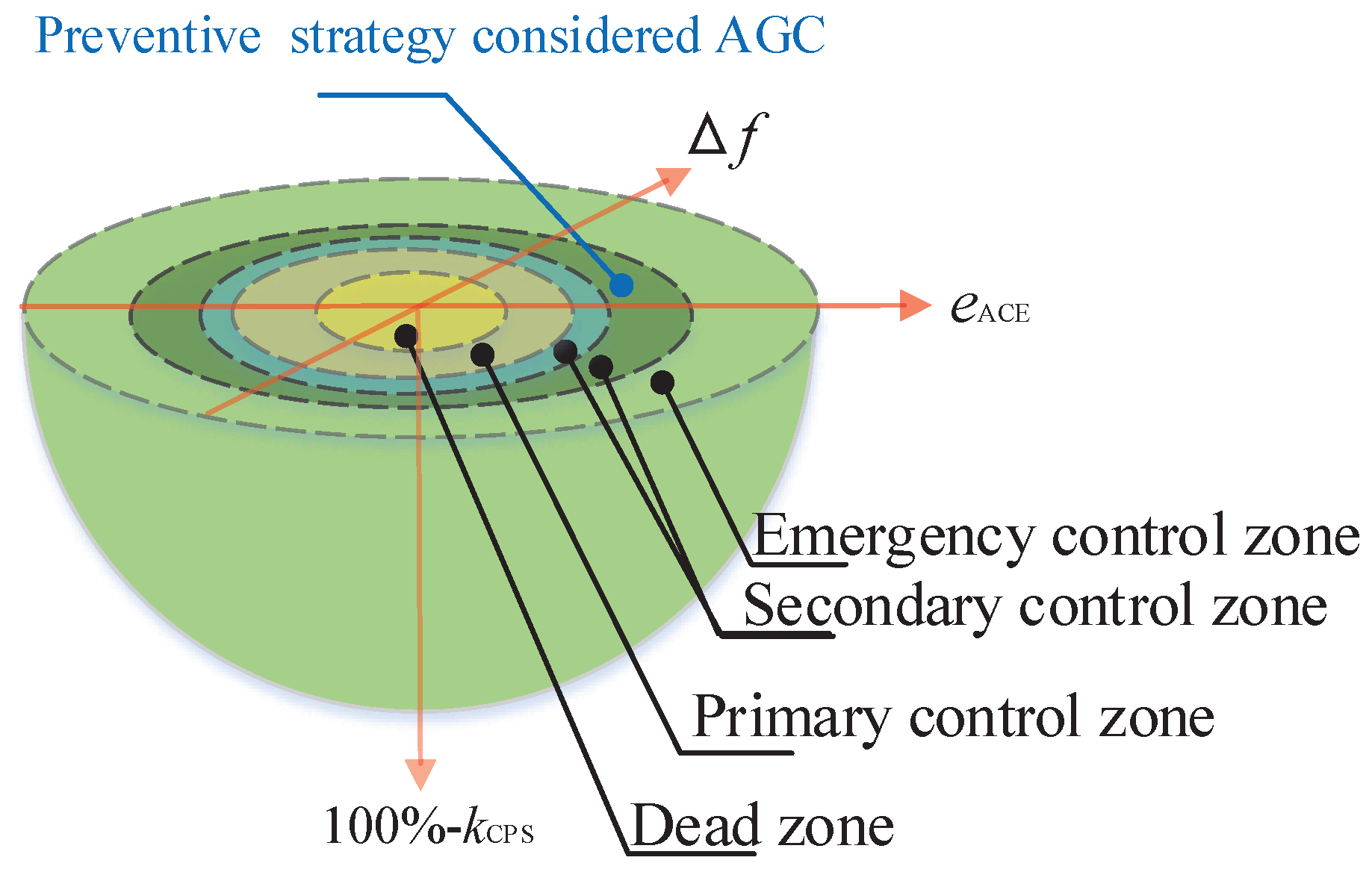
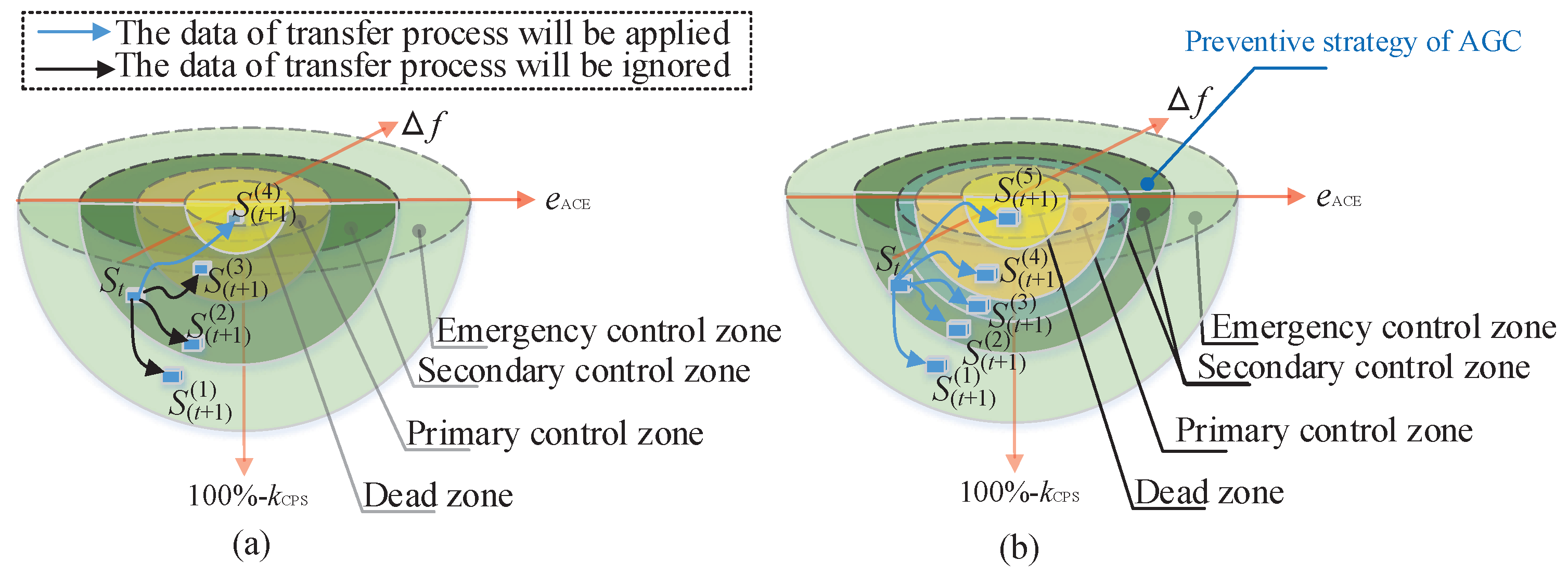
2.1. Emergency State

AGC not only aims to balance the active power between generators and system loads in a large-scale interconnected power system but is also designed to reduce the frequency deviation of the power system. That is to say, a high control performance of an AGC controller is significantly important for a control area to maintain the frequency deviation within normal levels.

Generally, frequency control has three gradations, i.e., a primary control zone, a secondary control zone, and an emergency control zone (see Figure 1). The primary control zone, which is subject to primary frequency regulation (PFR), is automatically regulated by the generator in response to frequency changes. The secondary control zone, which leads to AGC or secondary frequency regulation (SFR), is regulated by a control algorithm. The emergency control zone or tertiary control zone results in the implementation of economical dispatch and unit commitment, which occur with longer timescales, e.g., 15 min for economical dispatch (ED) and 24 h for unit commitment (UC). In particular, the range of the area control error (ACE) for each gradation is dependent on the basic capacity of the power system. Each gradation has a different frequency deviation range and a different control performance standard (CPS) index range:

• The range of the frequency deviation for the dead zone is from $(f_0-\Delta f_1)$ to $(f_0+\Delta f_1)$, where the frequency deviation $\Delta f_1$ is set to 0.025 Hz; The range of the CPS index for the dead zone is from $k_{\mathrm{CPS}\left(1\right)}$ to 100%, where the CPS index $k_{\mathrm{CPS}\left(1\right)}$ is set to 99% in this paper.
• The range of the frequency deviation for primary control is from $(f_0-\Delta f_2)$ to $(f_0+\Delta f_2)$, where the frequency deviation $\Delta f_2$ is set to 0.1 Hz; The range of the CPS index for primary control is from $k_{\mathrm{CPS}\left(2\right)}$ to $k_{\mathrm{CPS}\left(1\right)}$, where the CPS index $k_{\mathrm{CPS}\left(2\right)}$ is set to 95% in this paper.
• The range of the frequency deviation for secondary control is from $(f_0-\Delta f_3)$ to $(f_0+\Delta f_3)$, where the frequency deviation $\Delta f_3$ is set to 0.5 Hz; The range of the CPS index for secondary control is from $k_{\mathrm{CPS}\left(3\right)}$ to $k_{\mathrm{CPS}\left(2\right)}$, where the CPS index $k_{\mathrm{CPS}\left(3\right)}$ is set to 85% in this paper.
• The range of the frequency deviation for emergency control is from $(f_0-\Delta f_4)$ to $(f_0+\Delta f_4)$, where the frequency deviation $\Delta f_4$ is set to ∞ Hz; The range of the CPS index for emergency control is from $k_{\mathrm{CPS}\left(4\right)}$ to $k_{\mathrm{CPS}\left(3\right)}$, where the CPS index $k_{\mathrm{CPS}\left(4\right)}$ is set to 0% in this paper.

To minimize emergency situations for a power system when a large load suddenly occurs, a preventive strategy for AGC is described below. Frequency deviation ranges from $(f_0-\Delta f_3)$ to $(f_0-\Delta f_{\mathrm{e}})$ and from $(f_0+\Delta f_{\mathrm{e}})$ to $(f_0+\Delta f_3)$ were selected as the ranges for the preventive strategy. The preventive strategy aims to maintain the system frequency deviation $\Delta f$ at a minimum value, i.e., $\Delta f\to 0$ and $|\Delta f|<\Delta f_{\mathrm{e}}$. The frequency deviation for the preventive strategy $\Delta f_{\mathrm{e}}$ was set to 0.2 Hz in this study.

2.2. Framework of Automatic Generation Control

A basic AGC/LFC model contains two control areas. Each control area contains an AGC controller, a governor, a non-reheat turbine generator, and a system power flow load $\Delta P_{\mathrm{LA}}$ or $\Delta P_{\mathrm{LB}}$ [33]. Three major features required for the AGC controller in an interconnected power system can be summarized as follows.

• The controller should provide generation commands to the AGC unit to balance the real-time active power flow between the generator and system loads;
• The controller should reduce the frequency deviation in the control area;
• The controller should decrease the scheduled tie-line power deviation between any two areas, i.e., mitigate the value of the ACE.

Therefore, the frequency deviation $\Delta f$, the ACE $e_{\mathrm{ACE}}$, the scheduled tie-line power deviation $\Delta P_{\mathrm{T}}$, CPS indices (including CPS index $k_{\mathrm{CPS}}$, CPS1 index $k_{\mathrm{CPS}1}$, and CPS2 index $k_{\mathrm{CPS}2}$) are the inputs to the AGC controller. The generation command provided to the AGC unit is then the output of the controller.

2.3. Control Objective of Automatic Generation Control

In each control area, the AGC controller aims to (i) minimize the systemic frequency deviation $\Delta f$, (ii) reduce the value of the ACE $e_{\mathrm{ACE}}$, and (iii) maximize the CPS index $k_{\mathrm{CPS}}$.

The value of the ACE $e_{\mathrm{ACE}}$ can be calculated as

$$e_{\mathrm{ACE}}=\Delta P_{\mathrm{t}}-10B\Delta f,$$

(1)

where $\Delta P_{\mathrm{t}}$ is the scheduled tie-line power deviation; B is the frequency response coefficient of the control area (in MW/0.1 Hz); $\Delta f$ is the frequency deviation (in Hz).

The CPS index $k_{\mathrm{CPS}}$, which includes CPS1 index and CPS2 index, is established by the North American Electric Reliability Council (NERC) [12,34,35]. The CPS index is the statistic index of $\Delta f$ and $e_{\mathrm{ACE}}$ over a long period of time, rather than the real-time values of $\Delta f$ and $e_{\mathrm{ACE}}$. The CPS index $k_{\mathrm{CPS}}$ can be calculated as

$$k_{\mathrm{CPS}}(\%)=\left(\frac{N_{{\alpha }_{\mathrm{CF}}=1}}{N_{{\alpha }_{\mathrm{CF}}=1}+N_{{\alpha }_{\mathrm{CF}}=0}}\right)\times 100\%,$$

(2)

where $N_{{\alpha }_{\mathrm{CF}}=1}$ is the number of periods when ${\alpha }_{\mathrm{CF}}=1$; $N_{{\alpha }_{\mathrm{CF}}=0}$ is the number of periods when ${\alpha }_{\mathrm{CF}}=0$. The variable ${\alpha }_{\mathrm{CF}}$ can be calculated as

$${\alpha }_{\mathrm{CF}}=\left\{\begin{array}{c}1,\left\{\begin{array}{c}{\alpha }_{\mathrm{CF}1}\ge 200\%\hfill \\ 100\%\le {\alpha }_{\mathrm{CF}1}\le 200\%,{\alpha }_{\mathrm{CF}2}=1\hfill \end{array}\right.\hfill \\ 0,\left\{\begin{array}{c}{\alpha }_{\mathrm{CF}1}<100\%\hfill \\ 100\%\le {\alpha }_{\mathrm{CF}1}\le 200\%,{\alpha }_{\mathrm{CF}2}=0\hfill \end{array}\right.\hfill \end{array}\right.,$$

(3)

where ${\alpha }_{\mathrm{CF}1}$ and ${\alpha }_{\mathrm{CF}2}$ can be calculated as follows.

$${\alpha }_{\mathrm{CF}1}=\frac{E_{\mathrm{AVE}-1\min }\Delta F_{\mathrm{AVE}-1\min }}{-10B{\epsilon }_{1\min }^2},$$

(4)

$${\alpha }_{\mathrm{CF}2}=\frac{E_{\mathrm{AVE}-10\min }}{16.5{\epsilon }_{10min}\sqrt{B_{\mathrm{s}}B}},$$

(5)

where $E_{\mathrm{AVE}-1\min }$ is the clock-1-min average of the ACE; $E_{\mathrm{AVE}-10\min }$ is the the clock-10-min average of the ACE; $\Delta F_{\mathrm{AVE}-1\min }$ is the clock-1-min average of the frequency deviation; ${\epsilon }_{1\min }$ is the targeted frequency bound for the CPS1 index with clock-1-min; ${\epsilon }_{10\min }$ is the targeted frequency bound for the CPS1 index with clock-10-min; B represents the frequency bias of the control area, expressed in MW/0.1 Hz; $B_{\mathrm{S}}$ represents the frequency bias of the power system, expressed in MW/0.1 Hz.

Furthermore, the CPS1 index evaluates the impact of the ACE deviation on the frequency of system, while the CPS2 index is used to restrict the ACE magnitude. They can be calculated as follows:

$$k_{\mathrm{CPS}1}=(2-{\left\{{\alpha }_{\mathrm{CF}1}\right\}}_T)\times 100\%,$$

(6)

$$k_{\mathrm{CPS}2}=(\frac{N_{{\alpha }_{\mathrm{CF}2}<1}}{N_{{\alpha }_{\mathrm{CF}2}<1}+N_{{\alpha }_{\mathrm{CF}2}\ge 1}})\times 100\%,$$

(7)

where ${\left\{{\alpha }_{\mathrm{CF}1}\right\}}_T$ is the average value of the variable ${\alpha }_{\mathrm{CF}1}$ at the period of T, which is always 1 year; $N_{{\alpha }_{\mathrm{CF}2}<1}$ is the number of periods when ${\alpha }_{\mathrm{CF}2}<1$; $N_{{\alpha }_{\mathrm{CF}2}\ge 1}$ is the number of periods when ${\alpha }_{\mathrm{CF}2}\ge 1$.

3. Deep Forest Reinforcement Learning and Preventive Strategy

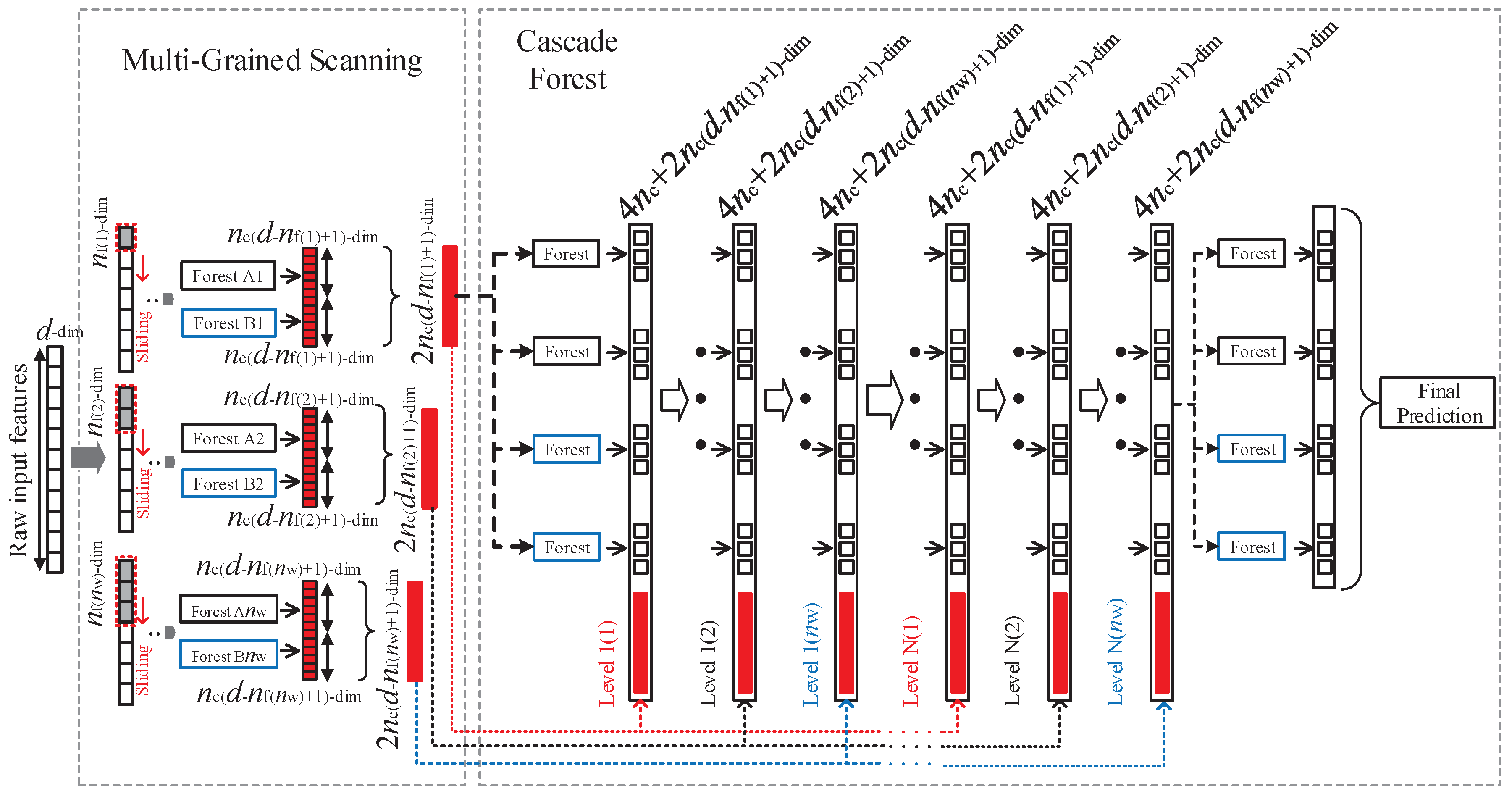
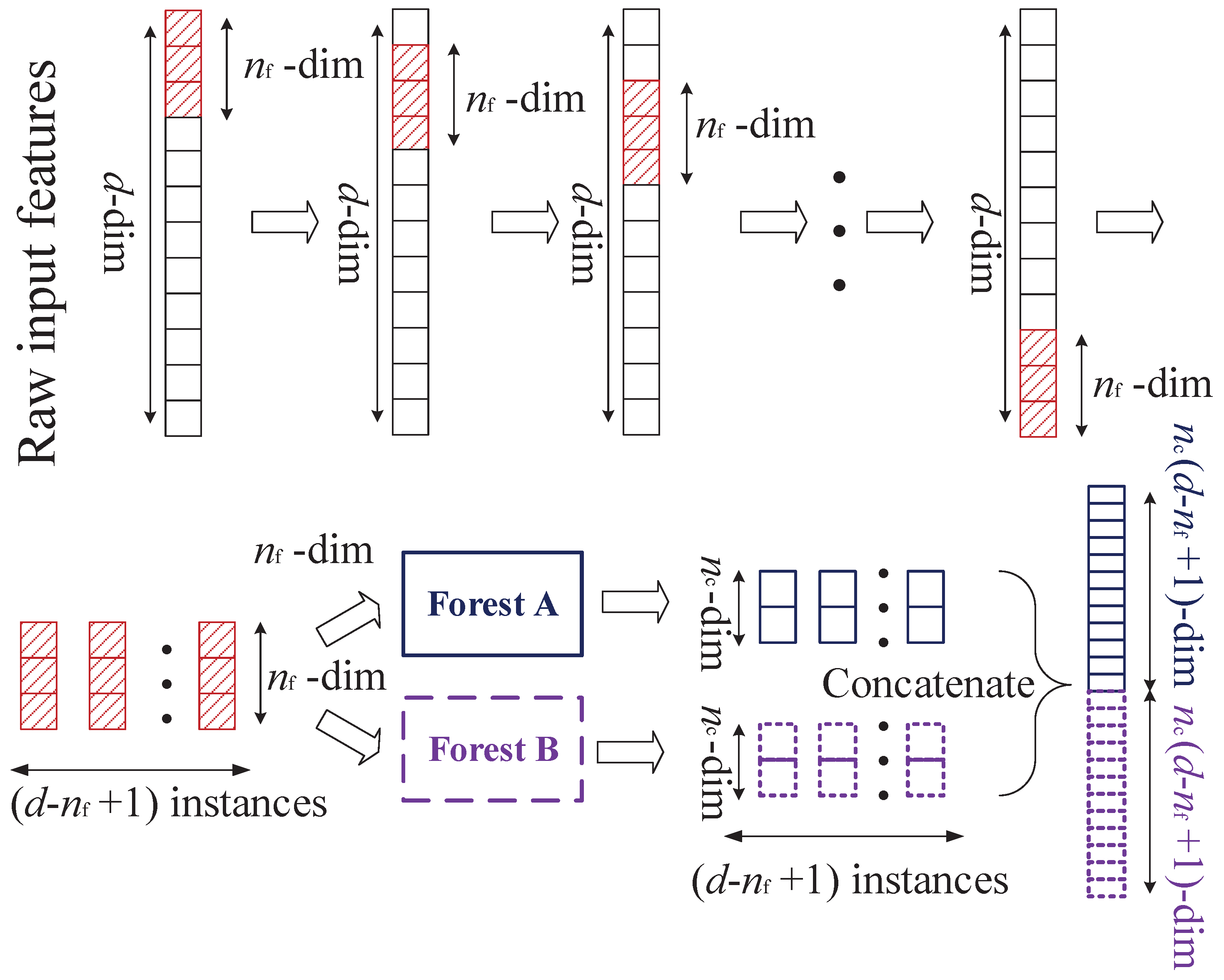
3.1. Deep Forest

As a decision tree ensemble algorithm, deep forest can perform representation learning [27]. Actually, deep forest contains two procedures, i.e., cascade forest structure and multi-grained scanning (Figure 2).

In the cascade forest structure procedure, deep forest cascades decision tree forests level-by-level. The input of each level is the feature information and is processed by the preceding level. The cascade forest structure of deep forest includes two types of forests, i.e., two completely-random tree forests (‘Forest A’) and two random forests (‘Forest B’) [27]. Both types of forests contain 500 trees. The completely random trees, which randomly select a feature to split at each node of the tree, will stop growing if each leaf node contains only the same classes of instances. The model of a random forest is an ensemble algorithm, which contains a group of decision tree classifiers $\{h(\mathbf{X},{\mathsf{\Theta }}_k)\}$, where k = 1, 2, …, $n_{\mathrm{c}}$; $n_{\mathrm{c}}$ is the number of classes; ${\mathsf{\Theta }}_k$ is a random vector; ${\mathsf{\Theta }}_k$ and the kth decision tree are independent with the same distribution. Then, the class that obtains the maximum vote is the right class to use for prediction,

$$H\left(x\right)=arg\underset{Y}{max}\sum _{i=1}^{N}I(h_i\left(x\right)=Y),$$

(8)

where x is a sample; $h_i\left(x\right)$ is the classification model of the ith decision tree; Y is the target classes; and $I(•)$ is the indicator function.

The random trees randomly select $\lfloor \sqrt{d}\rfloor$ features as candidates and then choose the one with the best Gini coefficient for splitting, where d is the number of input features, and $\lfloor d\rfloor$ rounds d to the nearest integer that is less than or equal to d. The Gini coefficient G can be calculated as

$$G=1-\sum _{i=1}^{n_{\mathrm{c}}}{\left[p(i|t)\right]}^2,$$

(9)

where $p(i|t)$ is the conditional probability of the ith class given the tth class; $n_{\mathrm{c}}$ is the number of samples. All the samples are of the same class when the Gini coefficient $G=0$. When the set C is split into subset $C_1$ and subset $C_2$, the split of the Gini coefficient index $G_{\mathrm{split}}\left(C\right)$ can be calculated as

$$G_{\mathrm{split}}\left(C\right)=\frac{n_1}{n}G(C_1)+\frac{n_2}{n}G(C_2),$$

(10)

where $n_1$ and $n_2$ are the number of samples of subset $C_1$ and subset $C_2$, respectively. To obtain the average of the final class vector, each instance should be trained $k-1$ times with k-fold cross-validation. The training performance of the whole cascade forest is estimated based on the validation set when a new level cascade is expanded. The total number of levels N is determined when the significant performance stops increasing.

In the multi-grained scanning procedure: (I) sliding windows are applied to scan the raw features of the input information; (II) an $n_{\mathrm{f}}$-dimensional feature vector is generated by the scanning window for each feature if a window size of $n_{\mathrm{f}}$ features is selected (Figure 3); (III) $(d-n_{\mathrm{f}}+1)$ feature vectors are produced as transformed features for ‘Forest A’ and ‘Forest B’; (IV) a $2n_{\mathrm{c}}(d-n_{\mathrm{f}}+1)$-dim transformed feature vector is produced for the inputs of the cascade forest structure if the number of classes is $n_{\mathrm{c}}$.

For example: (I) $n_{\mathrm{f}}\left(1\right)$, $n_{\mathrm{f}}\left(2\right)$, and $n_{\mathrm{f}(n_{\mathrm{w}})}$ sizes of sliding windows are applied to scan the d-dim raw features (Figure 2) if the number of classes is $n_{\mathrm{c}}$ and the number of sliding windows is $n_{\mathrm{w}}$; (II) $n_{\mathrm{w}}$ × $2n_{\mathrm{c}}(d-n_{\mathrm{f}}+1)$-dim transformed feature vectors are produced by the multi-grained scanning procedure for the cascade forest; (III) the deep forest cascade has $N·n_{\mathrm{c}}$ levels of forests, where each $n_{\mathrm{c}}$ level has $4n_{\mathrm{c}}+2n_{\mathrm{c}}(d-n_{\mathrm{f}}(1)+1)$, $4n_{\mathrm{c}}+2n_{\mathrm{c}}(d-n_{\mathrm{f}}\left(2\right)+1)$, …, $4n_{\mathrm{c}}+2n_{\mathrm{c}}(d-n_{\mathrm{f}(n_{\mathrm{w}})}+1)$ dimensional features, respectively, where $4n_{\mathrm{c}}$-dim features are 4 (2 ‘Forest A’ + 2 ‘Forest B’) times the $n_{\mathrm{c}}$-dim class vector; N is the number of each $n_{\mathrm{w}}$ level; (IV) the deep forest terminates model complexity training when adequate.

Compared to the deep neural networks in [27], deep forest can obtain a higher performance with low-dimensional data, while deep neural networks perform well for high-dimensional data. In [27], convolutional neural networks, machine learning practical, random forest, support vector machine, and k-nearest neighbors algorithms were compared to deep forest using low-dimensional data. The results of these comparisons showed that the other deep learning algorithms have many hyperparameters and a higher performance for high-dimensional data. Meanwhile, the prediction of the next systemic state in the AGC problem is a problem with low-dimensional data.

3.2. Reinforcement Learning

As one of the most famous methods for reinforcement learning, Q learning is a model-free control algorithm. The framework of Q learning contains a controller and an environment. The Q learning-based controller can update its strategy for an environment online. The inputs of the controller are the state value and reward value, while the output is an action for the environment. A controller that is based on Q learning provides an action a at the current state s in an environment based on the Q-value matrix $\mathbf{Q}$ and probability distribution matrix $\mathbf{P}$. These two matrices can be subsequently updated as

$$Q(s,a)\leftarrow Q(s,a)+\alpha (R(s,s^{\prime },a)+\gamma \underset{a\in A}{max}Q(s^{\prime },a)-Q(s,a)),$$

(11)

$$P(s,a)\leftarrow \left\{\begin{array}{cc}P(s,a)-\beta (1-P(s,a)),\hfill & \mathrm{if}{a}^{\prime }=a\hfill \\ P(s,a)(1-\beta ),\hfill & \mathrm{Otherwise}\hfill \end{array}\right.,$$

(12)

where $\alpha$ is the learning rate of Q learning; $\gamma$ is the discount coefficient of Q learning; $\beta$ is the probability coefficient of Q learning; s and $s^{\prime }$ are the current state and the next state of the environment, respectively; $R(s,s^{\prime },a)$ is the reward function obtained from the current state s to the next state $s^{\prime }$ with a selected action a. Both the current state s and the next state $s^{\prime }$ belong to the state set $\mathbf{S}$, i.e., $s\in \mathbf{S}$ and $s^{\prime }\in \mathbf{S}$. The selected action a belongs to the action set $\mathbf{A}$, i.e., $a\in \mathbf{A}$.

A particular process in the AGC problem of a interconnected power system is: the frequency deviation $\Delta f$ and the ACE are set to states; the generation command $\Delta P$ is set to an action; the parameters of Q learning for the simulation described in this paper are given in Appendix A.

The action for the output is selected by the given strategy, which should balance the exploration and the exploitation of the search of the action space. Generally, a greedy strategy for action selection always selects the maximum probability from the probability distribution matrix. Thus, the exploration for a selection is lost using the greedy strategy. Therefore, a selection strategy with both exploration and exploitation is applied to select an action from the action set. The selected action for the next iteration $a^{\prime }$ is selected by a random probability $p_{\mathrm{rand}}$ and the probability distribution matrix. The constraint of action selection can be described as follows:

$$\sum _{i=1}^{1+arg\left(a^{\prime }\right)}{P}_{s^{\prime },i}>p_{\mathrm{rand}}\ge \sum _{i=1}^{arg\left(a^{\prime }\right)}{P}_{s^{\prime },i},$$

(13)

where $arg\left(a^{\prime }\right)$ is the index number of the selected action $a^{\prime }$ in the action set.

Since the states and actions of Q learning are discrete values, the number of states in the state set and the number of actions in the action set should be increased to improve the accuracy of Q learning. Thus, to arrive at the optimal policy, the calculation memory of the state set and the action set of Q learning should be increased. In particular, Q learning can be applied to discrete control processes, such as AGC, whose control period is 4 s. Furthermore, to obtain higher convergence speed, other reinforcement learning algorithms have been employed for the AGC controller, such as, Q($\lambda$) learning [14] and R($\lambda$) learning [15]. Since the controller based on these reinforcement learning algorithms can update the control strategy online without knowing the model of the control object, the controller based on these reinforcement learning algorithms can obtain a high control performance in delay dynamic systems, such as large-scale interconnected power systems.

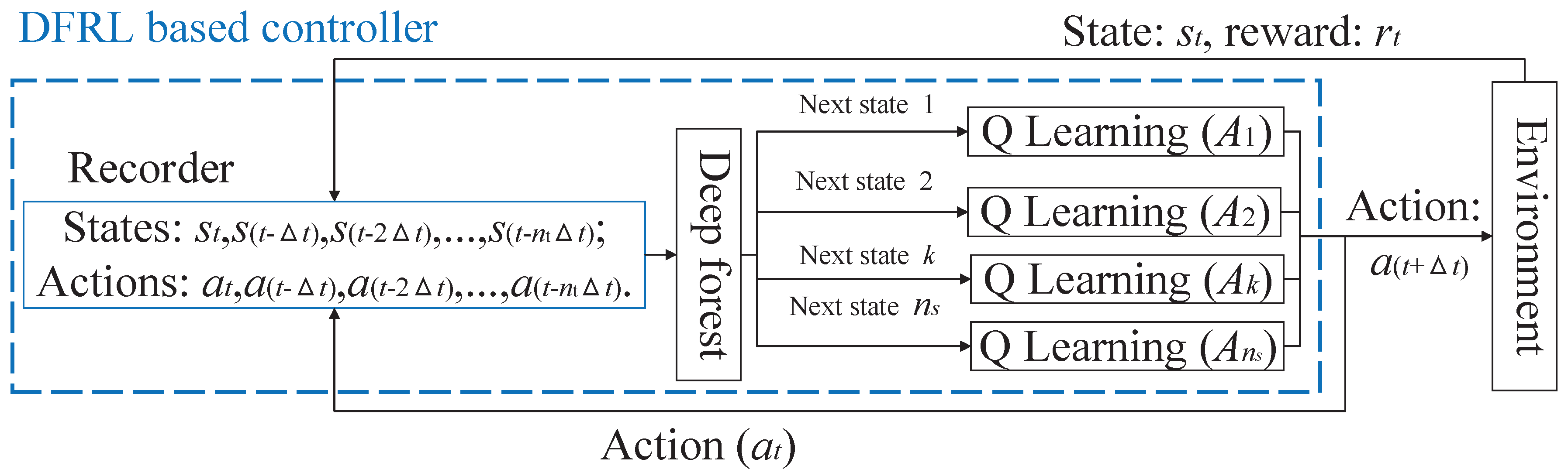
3.3. Deep Forest Reinforcement Learning

To obtain a more accurate control performance, the number of states and the number of actions in the action set of a conventional reinforcement learning should be increased. However, to reduce the effect of the curse of dimensionality, which leads to calculation memory error, the number of states and the number of actions in the action set of reinforcement learning should be reduced. To obtain a more accurate control performance and simultaneously reduce the curse of dimensionality, a DFRL algorithm is proposed in this paper.

The DFRL-based controller contains a recorder for diachronic states and actions, deep forest, and Q learning frameworks (Figure 4). To reduce the memory of calculation, the Q-value matrix $\mathbf{Q}$ and the probability distribution matrix $\mathbf{P}$ of Q learning are split into a total of $n_{\mathrm{s}}$ Q-value matrices and $n_{\mathrm{s}}$ probability distribution matrices, respectively. Thus, the calculation memory for matrix $\mathbf{Q}$ and matrix $\mathbf{P}$ can be reduced by $\frac{1}{n_{\mathrm{s}}}$,

$$\eta =\frac{{\displaystyle \sum _{i=1}^{n_{\mathrm{s}}}}{(\frac{n_{\mathrm{q}}}{n_{\mathrm{s}}})}^2}{n_{\mathrm{q}}^2}=\frac{n_{\mathrm{s}}{(\frac{n_{\mathrm{q}}}{n_{\mathrm{s}}})}^2}{n_{\mathrm{q}}^2}=\frac{1}{n_{\mathrm{s}}},$$

(14)

if both matrix $\mathbf{Q}$ and matrix $\mathbf{P}$ are $n_{\mathrm{q}}\times n_{\mathrm{q}}$ matrices, and if they are symmetrically split into two $\frac{n_{\mathrm{q}}}{n_{\mathrm{s}}}\times \frac{n_{\mathrm{q}}}{n_{\mathrm{s}}}$ matrices. Therefore, the curse of dimensionality of the framework of Q learning can be reduced by $\frac{1}{n_{\mathrm{s}}}$. For instance, $n_{\mathrm{s}}$ is set to 3 in the simulations reported in this paper; thus, the curse of dimensionality of the framework of Q learning can be reduced by ${\displaystyle \frac{1}{3}}$.

In the framework of conventional Q learning, the immediate state $S_t$, which is the state of the t-th time, is applied to represent a power system. However, in the framework of the DFRL, both the diachronic states and the diachronic actions are utilized to represent a power system. The major reasons are that (i) the power system is a time-delay system and (ii) diachronic actions can affect the state of the power system. Therefore, deep forest is applied to represent the next state of a power system with diachronic states and diachronic actions. Consequently, the inputs to the deep forest are the diachronic states of the environment and the diachronic actions of the DFRL -based controller, while the output of the deep forest is the next state of the power system.

The major features of the proposed DFRL-based controller can be summarized as

• Since the calculation memory is reduced because of the split matrices $\mathbf{Q}$, $\mathbf{P}$, and $\mathbf{A}$, the curse of dimensionality is reduced and a more accurate control performance can be obtained; thus, the number of actions in the action set and the number of states in the state set of the reinforcement learning of DFRL can be increased to obtain an accurate control action.
• The next systemic state can be predicted more accurately by the deep forest of DFRL with diachronic states and actions.

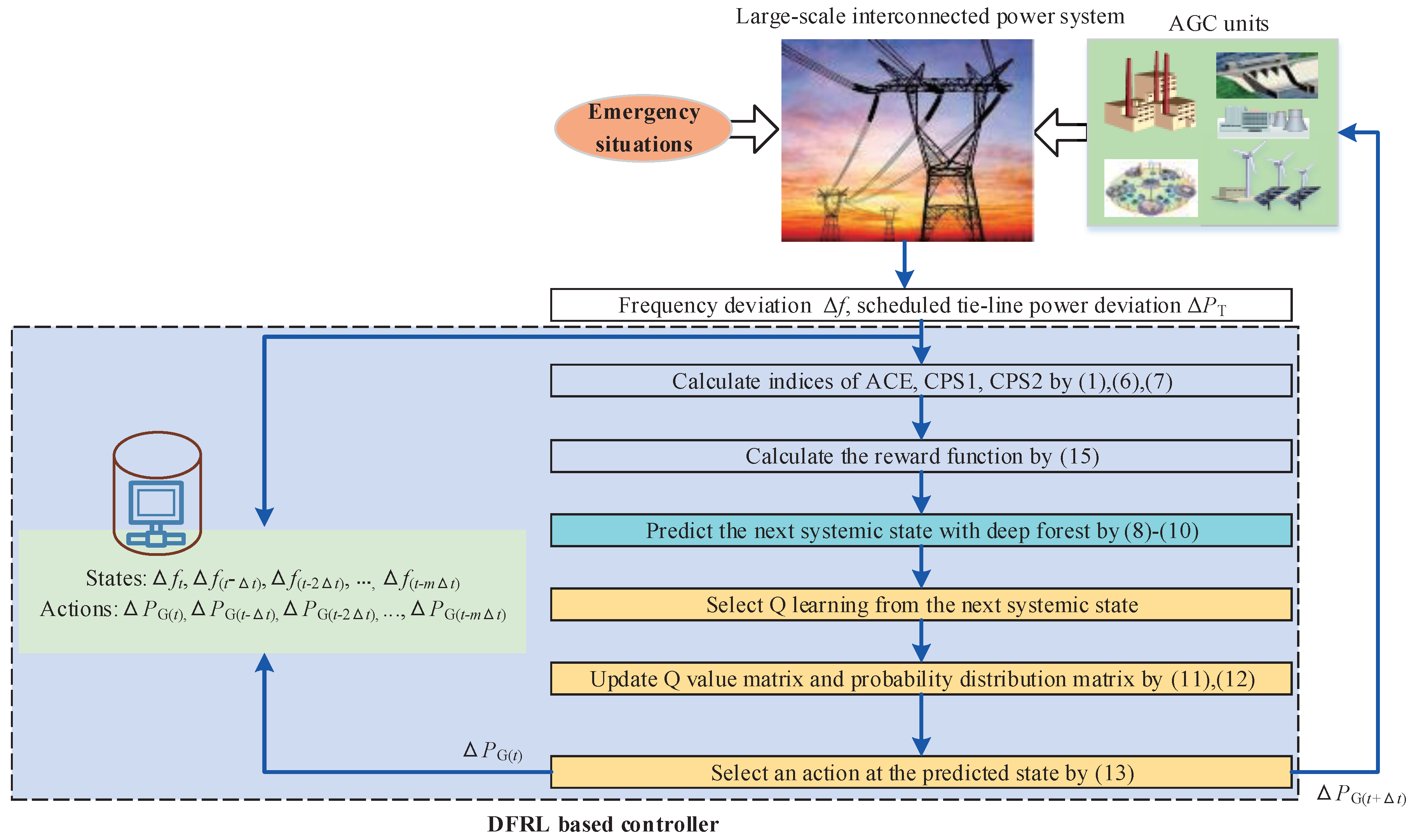
3.4. Deep Forest Reinforcement Learning as a Preventive Strategy for Automatic Generation Control

In the framework of the DFRL-based controller as a preventive strategy for AGC, the Q-value matrix is split into three submatrices, i.e., $n_{\mathrm{s}}$ = 3. The number of classes of next states is three, depending on the frequency deviation $\Delta f$, i.e., RL-I for $(-\infty ,-0.1]$ Hz, RL-II for $(-0.1,0.1]$ Hz, and RL-III for $(0.1,\infty )$ Hz. The control period of the controller of the preventive strategy for AGC is set to 4 s, i.e., $\Delta t$ = 4 s. The current state of the environment $S_t$ is defined as the frequency deviation of the power system $\Delta f_t$, i.e., $S_t=\Delta f_t$. The action at the t-th time of the power system $a_t$ is defined as the generation command for the AGC unit at the t-th time $\Delta P_{\mathrm{G}t}$, i.e., $a_t=\Delta P_{\mathrm{G}t}$ (Figure 5). The reward value $r_t$ for the reward function can be described as

$$r_t=R(s,s^{\prime },a)=\left\{\begin{array}{cc}{\lambda }_1,\hfill & \left|\Delta f_t\right|\le \Delta f_{\mathrm{s}0}\hfill \\ {\lambda }_2\Delta {f_t}^2,\hfill & \mathrm{Otherwise}\hfill \end{array}\right.,$$

(15)

where the reward value $r_t$ is a positive value ${\lambda }_1$ when $|\Delta f_t|$ is less than or equal to $\Delta f_{\mathrm{s}0}$; ${\lambda }_1>0$, ${\lambda }_2<0$, and $\Delta f_{\mathrm{s}0}<0.1\mathrm{Hz}$. The variables ${\lambda }_1$, ${\lambda }_2$, $\Delta f_{\mathrm{s}0}$ in this work were set to 10, −100, and 0.005 Hz, respectively. The pseudo-code of the proposed DFRL for the preventive strategy for AGC is given in Algorithm 1.

Algorithm 1 Pseudo-code of the proposed deep forest reinforcement learning for the preventive strategy for automatic generation control
1:	Initial parameters of Q learning of the DFRL, i.e., $\alpha ,\gamma ,\beta$
2:	Initial system state s
3:	Initial Q-value matrix $\mathbf{Q}$ and probability distribution matrix $\mathbf{P}$
4:	while loop: do
5:	Obtain the system state s from the environment as Equations (1), (6), and (7)
6:	Save the system state s to the recorder of the DFRL
7:	Calculate the reward value $R(s,s^{\prime },a)$ as Equation (15)
8:	Select Q learning from the next systemic state as Equations (8)–(10)
9:	Update Q-value matrix and probability distribution matrix as Equations (11) and (12), respectively
10:	Select the output action by $\mathbf{P}$ and a random probability as Equation (13)
11:	Given the selected output action to the AGC unit and the recorder of the DFRL
12:	return loop

3.5. Pre-Training Process of Deep Forest Reinforcement Learning

DFRL and reinforcement learning are data-hungry algorithms. Generally, in the pre-training process of a reinforcement learning algorithm, the higher the control performance of the training data, the higher the convergence speed obtained. However, DFRL needs all the training data, including training data with high and low control performance. The training data of DFRL originated from the simulation data of reinforcement learning in this work. In the training process of conventional reinforcement learning, training data with a low control performance are ignored (Figure 6a). However, in the training process of DFRL, training data with both high and low control performances are applied to the deep forest for learning the dynamic system (Figure 6b). Furthermore, the more training data, the higher the control performance obtained by DFRL. Consequently, the major reasons that training data with high and low control performances can be applied to DFRL can be summarized as (i) the more data, which includes data with high and low control performances, the more state spaces of the power system covered; (ii) the more data, the more accurate the representation of DFRL obtained.

4. Case Study

The MATLAB/Simulink models and programs of the power system models in this study were developed in an Intel Core 8 Duo processor of a 2.4 GHz and 8 GB RAM computer with MATLAB version 9.1.0 (R2016b).

The number of forests in the multi-grained scanning and the cascade of DFRL were set to 2 and 8 as default settings, respectively. The number of trees in each forest of DFRL was set to 500 as a default. A larger number for $n_{\mathrm{t}}$ means that more diachronic actions and states are recorded for the deep forest of DFRL and more calculation time. After extensive training, both the number of diachronic actions and states in this paper were set to 10, i.e., $n_{\mathrm{t}}$ = 10. The average calculation time of each iteration of DFRL is 0.423 s when the number for $n_{\mathrm{t}}$ is set to 10. Also, the prediction results with $n_{\mathrm{t}}$ = 10 are the same as the prediction results with $n_{\mathrm{t}}$ = 30, while the average calculation time of each iteration of DFRL is 1.862 s when this number $n_{\mathrm{t}}$ = 30. The dimensions of the raw features were double the value of $n_{\mathrm{t}}$, i.e., $d=2n_{\mathrm{t}}=20$. Sliding window sizes were set to {$\lfloor d/8\rfloor$, $\lfloor d/4\rfloor$, $\lfloor d/2\rfloor$}, i.e., {2, 5, 10}. The maximum depth of each tree growth was 100. Since the number of classifications of the next state $n_s$ was set to three, three subsidiary reinforcement learning algorithms were employed for DFRL. The learning rate $\alpha$ of these subsidiary reinforcement learning algorithms was set to 0.1 in this study; the value range of the learning rate should be $\alpha \in (0,1)$; a small learning rate means a slow learning speed, and a small learning rate is suitable for application; a large learning rate means a high learning speed, while a large learning rate is suitable for offline training. Two different learning rates were configured for Q learning in [14], and a dynamic learning rate strategy was proposed by Junhong Nie and Simon Haykin [36]. The discounted rate of reward $\gamma$ of these subsidiary reinforcement learning algorithms was set to 0.9 in this simulation. The value range of the discounted rate was set to $\gamma \in (0,1]$. A larger discounted rate means greater importance of the Q-value history. The constant of the probability distribution $\beta$ of these subsidiary reinforcement learning algorithms were set to 0.05. A large value of $\beta$ means a high speed for updating the selection probability.

The total states of these reinforcement learning algorithms (i.e., RL-I, RL-II, and RL-III) of DFRL cover from $-\infty$ to ∞ (

Table 1. State ranges and action sets of RL-I, RL-II, and RL-III.

Pow. ${}^{\mathbf{a}}$	Stat. ${}^{\mathbf{b}}$	Value
All	StaI. ${}^{\mathrm{d}}$	$\left\{\begin{array}{c}\Delta f:(-\infty ,-0.50,-0.46,-0.42,-0.38,-0.34,-0.30,-0.26,-0.22,-0.18,-0.14,-0.10]\mathrm{Hz}\hfill \\ k_{\mathrm{CPS}}:[0,70,80,82,84,86,88,90,92,93,94,95]\%\hfill \\ e_{\mathrm{ACE}}:\left\{\begin{array}{c}2-\mathrm{area}:[-10,-20,-30,-40,-50,-60,-70,-80,-90,-100,-110)(\mathrm{MW})\hfill \\ 3-\mathrm{area}:[-333,-633,-933,-1233,-1533,-1833,-2133,-2433,-2733,-3033,-3333)(\mathrm{MW})\hfill \\ 4-\mathrm{area}:[-567,-623,-680,-737,-793,-850,-907,-963,-1020,-1077,-1133)(\mathrm{MW})\hfill \end{array}\right.\hfill \end{array}\right.$
All	StaII. ${}^{\mathrm{d}}$	$\left\{\begin{array}{c}\Delta f:(-0.10,-0.08,-0.06,-0.04,-0.02,0.00,0.02,0.04,0.06,0.08,0.10]\mathrm{Hz}\hfill \\ k_{\mathrm{CPS}}:(95,96,97,98,99,99.5,99.5,99,98,97,96,95)\%\hfill \\ e_{\mathrm{ACE}}:\left\{\begin{array}{c}2-\mathrm{area}:(10,8,6,4,2,0,-2,-4,-6,-8,-10)(\mathrm{MW})\hfill \\ 3-\mathrm{area}:(333,267,200,133,67,0,-67,-133,-200,-267,-333)(\mathrm{MW})\hfill \\ 4-\mathrm{area}:(567,453,340,227,113,0,-113,-227,-340,-453,-567)(\mathrm{MW})\hfill \end{array}\right.\hfill \end{array}\right.$
All	StaIII. ${}^{\mathrm{d}}$	$\left\{\begin{array}{c}\Delta f:(0.10,0.14,0.18,0.22,0.26,0.30,0.34,0.38,0.42,0.46,0.50,\infty )\mathrm{Hz}\hfill \\ k_{\mathrm{CPS}}:[95,94,93,92,90,88,86,84,82,80,70,0]\%\hfill \\ e_{\mathrm{ACE}}:\left\{\begin{array}{c}2-\mathrm{area}:(110,100,90,80,70,60,50,40,30,20,10](\mathrm{MW})\hfill \\ 3-\mathrm{area}:(3333,3033,2733,2433,2133,1833,1533,1233,933,633,333](\mathrm{MW})\hfill \\ 4-\mathrm{area}:(1133,1077,1020,963,907,850,793,737,680,623,567](\mathrm{MW})\hfill \end{array}\right.\hfill \end{array}\right.$
2 ${}^{\mathrm{c}}$	ActI. ${}^{\mathrm{e}}$	{10, 19, 28, 37, 46, 55, 64, 73, 82, 91, 100}
2 ${}^{\mathrm{c}}$	ActII. ${}^{\mathrm{e}}$	{−10, −8, −6, −4, −2, 0, 2, 4, 6, 8, 10}
2 ${}^{\mathrm{c}}$	ActIII. ${}^{\mathrm{e}}$	{−100, −91, −82, −73, −64, −55, −46, −37, −28, −19, −10}
3 ${}^{\mathrm{c}}$	ActI. ${}^{\mathrm{e}}$	{300, 570, 840, 1110, 1380, 1650, 1920, 2190, 2460, 2730, 3000}
3 ${}^{\mathrm{c}}$	ActII. ${}^{\mathrm{e}}$	{−300, −240, −180, −120, −60, 0, 60, 120, 180, 240, 300}
3 ${}^{\mathrm{c}}$	ActIII. ${}^{\mathrm{e}}$	{−3000, −2730, −2460, −2190, −1920, −1650, −1380, −1110, −840, −570, −300}
4 ${}^{\mathrm{c}}$	ActI. ${}^{\mathrm{e}}$	{510, 561, 612, 663, 714, 765, 816, 867, 918, 969, 1020}
4 ${}^{\mathrm{c}}$	ActII. ${}^{\mathrm{e}}$	{−510, −408, −306, −204, −102, 0, 102, 204, 306, 408, 510}
4 ${}^{\mathrm{c}}$	ActIII. ${}^{\mathrm{e}}$	{−1020, −969, −918, −867, −816, −765, −714, −663, −612, −561, −510}

${}^{\mathrm{a}}$ Pow. = Power systems. ${}^{\mathrm{b}}$ Stat. = State ranges or action sets. ${}^{\mathrm{c}}$ 2 = Two-area (MW); ${}^{\mathrm{c}}$ 3 = Three-area (MW); ${}^{\mathrm{c}}$ 4 = China Southern Power Grid (MW). ${}^{\mathrm{d}}$ StaI. = State ranges (RL-I); StaII. = State ranges (RL-II); StaIII. = State ranges (RL-III). ${}^{\mathrm{e}}$ ActI. = Action set (RL-I); ActII. = Action set (RL-II); ActIII. = Action set (RL-III).

). These state range of these reinforcement learning algorithms are divided for AGC, which is a special discrete control system (Table 1). The optimal control for an ideal discrete control system based on AGC is one in which $\Delta P_i=-1\times e_{\mathrm{ACE}}$. The number of actions in the action set of each subsidiary reinforcement learning algorithm of DFRL was set to 11 (Table 1), which is according to [3]; thus, the total number of actions in these three subsidiary reinforcement learning algorithms of DFRL was 33, or 11 × 3; meanwhile, the number of actions in the action set of conventional reinforcement learning was set to 33.

Numerous conventional AGC algorithms are compared with the proposed algorithm for the preventive strategy for AGC in this paper, i.e., proportional–integral (PI), proportional–integral– differential (PID), sliding mode controller (SMC), active disturbance rejection control (ADRC), fractional-order PID (FOPID), fuzzy logic control (FLC), artificial neural network (ANN), Q learning, Q($\lambda$) learning, and R($\lambda$) learning. Both the DFRL and the conventional AGC algorithms were simulated for three power systems, i.e., IEEE two-area power system, three-area power system, and the China Southern Power Grid (Figure 7). The parameters of these conventional AGC algorithms are given in Appendix A. These parameters were obtained by genetic algorithm with a simple configuration, i.e., the population size was set to 100, and the maximum number of generations was set to 100.

Both conventional AGC algorithms and the proposed DFRL-based controller were applied to ‘Area A’ in these three power systems. The China Southern Power Grid contains four areas of China, i.e., ‘Area A’ for the Guangdong Power Grid, ‘Area B’ for the Guangxi Power Grid, ‘Area C’ for the Guizhou Power Grid, and ‘Area D’ for the Yunnan Power Grid [37]. In these three power systems: each control area contains a governor $1/(1+s{T}_{\mathrm{g}})$, a generator $1/(1+s{T}_{\mathrm{t}})$, and a frequency response model $K_{\mathrm{p}}/(1+s{T}_{\mathrm{p}})$; the frequency response coefficient and the droop coefficient are $B_i$ and $R_i$, respectively. Thus, the mathematical model of each generation unit can be described as follows.

$$G_{\mathrm{unit}}=\frac{1}{(1+s{T}_{\mathrm{g}})}\frac{1}{(1+s{T}_{\mathrm{t}})}$$

(16)

where $T_{\mathrm{g}}$ and $T_{\mathrm{t}}$ are the time constants of the governor and generator of each control area, respectively.

Also, the generation rate constraint $k_{\mathrm{GRC}}^i$ and adjustable capacity constraint $P_{max}^i$ are included in the real China Southern Power Grid model. In these three power systems, the ith area is connected to the jth area with the alternating current tie-line response model $2\pi T_{ij}/s$. The parameters of these three power systems are given in Appendix B, Appendix C and Appendix D, respectively. Two large continuous disturbances were designed for these power systems, i.e., ‘Case 1’ and ‘Case 2’ (Figure 8). These two large continuous disturbances may lead to the occurrence of emergency situations: (i) A large disturbance in the continuous coverage of all active power values represents the system load value space, as designed for ‘Case 1’. (ii) Since the power systems are delay systems, a large system load with delay was designed (‘Case 2’).

The control periods of the algorithms in all cases were set to 4 s, i.e., these algorithms were executed once every 4 s. The number of iterations of the training process of DFRL was set to 300 (Figure 9).

Simulation results show that the proposed DFRL method can obtain the best control performance with the smallest frequency deviation. The major reasons for this superior control performance are that: (i) the next state of a power system can be predicted by DFRL, such as the next states of the three-area power system in ‘Case 1’ (Figure 10); (ii) $\Delta f$ obtained by conventional Q learning may be larger than 0.03 Hz (Figure 10) when the next state of a power system lacks prediction. The calculation memory of Q learning is 17,688 Bytes, while that of DFRL is 6072 Bytes. Thus, compared to Q learning, the calculation memory of DFRL is reduced by 34.328% in these simulations. The training time for the deep forest of the DFRL algorithm is 35.14 min. The training time for the ANN, Q learning, Q($\lambda$) learning, and R($\lambda$) learning algorithms is less then 10 min.

The statistic simulation result obtained by the DFRL and conventional AGC algorithms is shown in

Table 2. Statistic simulation results.

Power Systems	Algorithms	$\Delta \mathit{f}$ (Hz)	${\mathit{e}}_{\mathbf{ACE}}$ (MW)	${\mathit{k}}_{\mathbf{CPS}}$ (%)
Two-area	PI	0.063	27	84.82
	PID	0.050	22	90.23
	SMC	0.081	35	85.54
	ADRC	0.056	24	82.34
	FOPID	0.066	28	83.29
	FLC	0.079	34	91.40
	ANN	0.065	28	91.06
	Q learning	0.091	39	77.72
	Q($\lambda$) learning	0.056	25	78.33
	R($\lambda$) learning	0.044	19	82.14
	DFRL	0.002	1	99.48
Three-area	PI	0.075	69	76.03
	PID	0.076	69	86.33
	SMC	0.184	192	67.24
	ADRC	0.095	65	78.66
	FOPID	0.188	209	78.78
	FLC	0.145	365	80.82
	ANN	0.133	88	83.87
	Q learning	0.091	83	81.41
	Q($\lambda$) learning	0.076	128	88.13
	R($\lambda$) learning	0.093	209	80.84
	DFRL	0.036	28	97.07
China Southern Power Grid	PI	0.072	237	80.43
	PID	0.049	203	82.49
	SMC	0.187	587	75.45
	ADRC	0.059	48	88.22
	FOPID	0.093	562	75.65
	FLC	0.084	568	75.62
	ANN	0.093	242	79.65
	Q learning	0.114	384	79.03
	Q($\lambda$) learning	0.111	443	77.23
	R($\lambda$) learning	0.111	256	78.36
	DFRL	0.041	62	92.23

and Figure 11. Note that, in Table 2 and Figure 11, the frequency deviation $\Delta f$ and ACE $e_{\mathrm{ACE}}$ are the average absolute values of all areas in all cases in the two-area power system, three-area power system, and four-area power system, respectively. Statistic simulation results (Table 2 and Figure 11) obtained by the DFRL and conventional AGC algorithms show that:

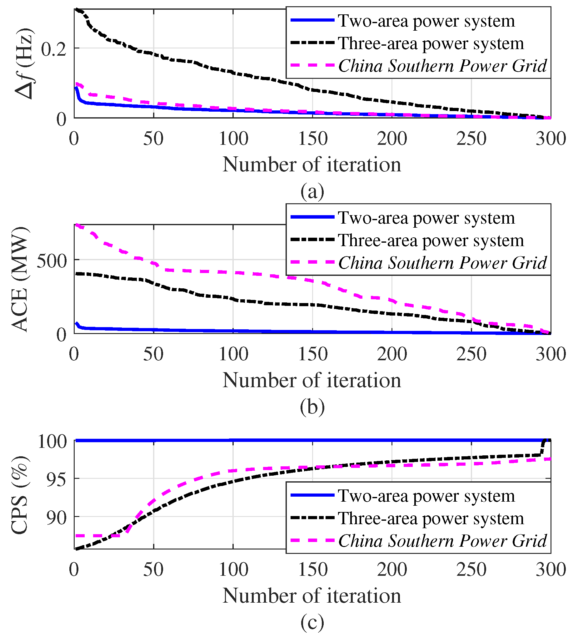
• The average absolute values of the frequency deviations obtained by DFRL are less than $\Delta f_2$ (i.e., 0.1 Hz), while the average absolute values of the frequency deviations obtained by 10 conventional AGC algorithms may larger than 0.1 Hz in both Case 1 and Case 2 (Table 2); Therefore, the emergency situation of a large-scale interconnected power system and the curse of dimensionality can simultaneously be reduced by the proposed DFRL.
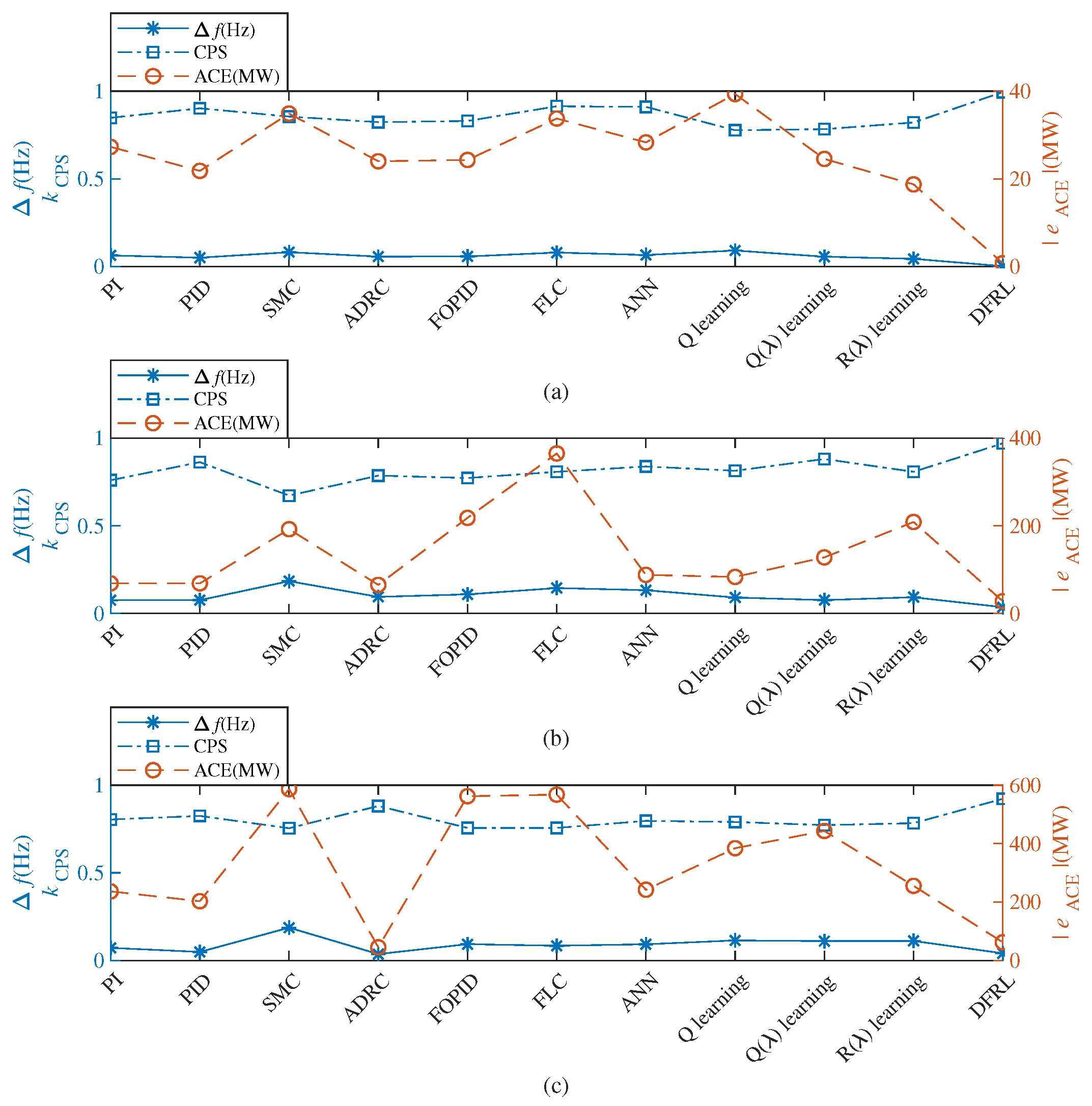
• Compared to 10 conventional AGC algorithms, DFRL can obtain the highest control performance with a smaller absolute value of frequency deviation $\Delta f$ and larger CPS index $k_{\mathrm{CPS}}$ (Figure 11).
• Since the deep forest of DFRL can perform representation learning for the states of the power system, the preventive strategy for AGC can be considered effective for a large-scale interconnected power system.

5. Conclusions

To reduce occurrences of emergency situations of power systems and mitigate the curse of dimensionality of reinforcement learning, a DFRL algorithm as a preventive strategy for AGC in large-scale interconnected power systems is proposed. Both the state set and action set of reinforcement learning are split into subsidiary reinforcement learning for mitigating the curse of dimensionality of reinforcement learning. A deep forest is then introduced to subsidiary reinforcement learning for forecasting the next state of the power system. Two cases of three power systems (i.e., two-area power system, three-area power system, and the China Southern Power Grid) with the DFRL and 10 conventional AGC algorithms were simulated in this work. The simulation results show that DFRL achieves the highest control performance. The major contributions of the DFRL algorithm can be summarized as follows:

• After the pre-training process using the data of reinforcement learning, the deep forest of DFRL can effectively forecast the next state of a power system. Different from the conventional applications of deep forest, the deep forest of DFRL is incorporated into the control algorithm;
• Since the subsidiary reinforcement learning algorithms of DFRL can update their strategies online, the DFRL can effectively provide generation commands to the controller as a preventive strategy for AGC in power systems. Compared to conventional AGC, the preventive strategy for AGC can predict the next systemic state of the power system;
• Since the next systemic state can be predicted and the calculation memory can be reduced by the DFRL method, the proposed DFRL-based controller can effectively reduce occurrences of emergency situations in large-scale interconnected power systems and simultaneously mitigate the curse of dimensionality. The conventional framework of reinforcement learning can be divided into multiple subsidiary structures for mitigating the curse of dimensionality.

References

1. Maleki, A.; Hafeznia, H.; Rosen, M.A.; Pourfayaz, F. Optimization of a grid-connected hybrid solar-wind-hydrogen CHP system for residential applications by efficient metaheuristic approaches. Appl. Therm. Eng. 2017, 123, 1263–1277. [Google Scholar] [CrossRef]
2. Allison, J. Robust multi-objective control of hybrid renewable microgeneration systems with energy storage. Appl. Therm. Eng. 2017, 114, 149–1506. [Google Scholar] [CrossRef]
3. Yin, L.; Yu, T.; Zhang, X.; Yang, B. Relaxed deep learning for real-time economic generation dispatch and control with unified time scale. Energy 2018, 149, 11–23. [Google Scholar] [CrossRef]
4. Yang, B.; Yu, T.; Shu, H.; Dong, J.; Jiang, L. Robust sliding-mode control of wind energy conversion systems for optimal power extraction via nonlinear perturbation observers. Appl. Energy 2018, 210, 711–723. [Google Scholar] [CrossRef]
5. Dahiya, P.; Sharma, V.; Naresh, R. Automatic generation control using disrupted oppositional based gravitational search spell optimized sliding mode controller under deregulated environment. IET Gener. Transm. Distrib. 2016, 10, 3995–4005. [Google Scholar] [CrossRef]
6. Liu, F.; Li, Y.; Cao, Y.; She, J.; Wu, M. A Two-Layer Active Disturbance Rejection Controller Design for Load Frequency Control of Interconnected Power System. IEEE Trans. Power Syst. 2016, 31, 3320–3321. [Google Scholar] [CrossRef]
7. Debbarma, S.; Saikia, L.C.; Sinha, N. Automatic generation control using two degree of freedom fractional order PID controller. Int. J. Electr. Power Energy Syst. 2014, 58, 120–129. [Google Scholar] [CrossRef]
8. Rahman, A.; Saikia, L.C.; Sinha, N. AGC of dish-Stirling solar thermal integrated thermal system with biogeography based optimized three degree of freedom PID controller. IET Renew. Power Gener. 2016, 10, 1161–1170. [Google Scholar] [CrossRef]
9. Jeyalakshmi, V.; Subburaj, P. PSO-scaled fuzzy logic to load frequency control in hydrothermal power system. Soft Comput. 2016, 20, 2577–2594. [Google Scholar] [CrossRef]
10. Nguyen, T.T.; Vu Quynh, N.; Duong, M.Q.; Van Dai, L. Modified Differential Evolution Algorithm: A Novel Approach to Optimize the Operation of Hydrothermal Power Systems while Considering the Different Constraints and Valve Point Loading Effects. Energies 2018, 11, 540. [Google Scholar] [CrossRef]
11. Nguyen, T.T.; Dinh, B.H.; Quynh, N.V.; Duong, M.Q.; Dai, L.V. A Novel Algorithm for Optimal Operation of Hydrothermal Power Systems under Considering the Constraints in Transmission Networks. Energies 2018, 11, 188. [Google Scholar] [CrossRef]
12. Yu, T.; Zhou, B.; Chan, K.W.; Chen, L.; Yang, B. Stochastic Optimal Relaxed Automatic Generation Control in Non-Markov Environment Based on Multi-Step Q(λ) Learning. IEEE Trans. Power Syst. 2011, 26, 1272–1282. [Google Scholar] [CrossRef]
13. Yu, T.; Wang, H.; Zhou, B.; Chan, K.; Tang, J. Multi-agent correlated equilibrium Q(λ) learning for coordinated smart generation control of interconnected power grids. IEEE Trans. Power Syst. 2015, 30, 1669–1679. [Google Scholar] [CrossRef]
14. Xi, L.; Yu, T.; Yang, B.; Zhang, X.; Qiu, X. A wolf pack hunting strategy based virtual tribes control for automatic generation control of smart grid. Appl. Energy 2016, 178, 198–211. [Google Scholar] [CrossRef]
15. Yu, T.; Zhou, B.; Chan, K.; Yuan, Y.; Yang, B.; Wu, Q. R(λ) imitation learning for automatic generation control of interconnected power grids. Automatica 2012, 48, 2130–2136. [Google Scholar] [CrossRef]
16. Watkins, C.J.C.H. Learning from Delayed Rewards. Ph.D. Thesis, Unpublished doctoral dissertation. Cambridge University, Cambridge, UK, 1989. [Google Scholar]
17. Yin, L.; Yu, T.; Zhou, L. Design of a Novel Smart Generation Controller Based on Deep Q Learning for Large-Scale Interconnected Power System. J. Energy Eng. 2018, 144, 04018033. [Google Scholar] [CrossRef]
18. Si, Y.L.; Jin, Y.G.; Yong, T.Y. Determining the Optimal Reserve Capacity in a Microgrid With Islanded Operation. IEEE Trans. Power Syst. 2015, 31, 1369–1376. [Google Scholar]
19. Hu-Ling, A.Y.; Fu-Suo, B.L.; Wei, T.C.L.; Guo-Yi, D.J.; Hao, E.H.; Hai-Bo, F.L.; Li, G.F. A coordination and optimization method of preventive control to improve the adaptability of frequency emergency control strategy in high-capacity generators and low load grid. In Proceedings of the 2014 International Conference on Power System Technology, Chengdu, China, 20–22 October 2014; pp. 485–490. [Google Scholar] [CrossRef]
20. Amani, A.M.; Gaeini, N.; Afshar, A.; Menhaj, M. A New Approach to Reconfigurable Load Frequency Control of Power Systems in Emergency Conditions. IFAC Proc. Vol. 2013, 46, 526–531. [Google Scholar] [CrossRef]
21. Bevrani, H.; Ledwich, G.; Ford, J.J.; Dong, Z.Y. On feasibility of regional frequency-based emergency control plans. Energy Convers. Manag. 2009, 50, 1656–1663. [Google Scholar] [CrossRef]
22. Sarker, B.R.; Faiz, T.I. Minimizing maintenance cost for offshore wind turbines following multi-level opportunistic preventive strategy. Renew. Energy 2016, 85, 104–113. [Google Scholar] [CrossRef]
23. Huang, G.; Wang, J.; Chen, C.; Qi, J.; Guo, C. Integration of Preventive and Emergency Responses for Power Grid Resilience Enhancement. IEEE Trans. Power Syst. 2017, 32, 4451–4463. [Google Scholar] [CrossRef]
24. Pertl, M.; Weckesser, T.; Rezkalla, M.; Heussen, K.; Marinelli, M. A decision support tool for transient stability preventive control. Electr. Power Syst. Res. 2017, 147, 88–96. [Google Scholar] [CrossRef] [Green Version]
25. Liu, W.; Qin, G.; He, Y.; Jiang, F. Distributed Cooperative Reinforcement Learning-Based Traffic Signal Control That Integrates V2X Networks’ Dynamic Clustering. IEEE Trans. Veh. Technol. 2017, 66, 8667–8681. [Google Scholar] [CrossRef]
26. Yin, L.; Yu, T.; Zhou, L.; Huang, L.; Zhang, X.; Zheng, B. Artificial emotional reinforcement learning for automatic generation control of large-scale interconnected power grids. IET Gener. Transm. Distrib. 2017, 11, 2305–2313. [Google Scholar] [CrossRef]
27. Zhou, Z.; Feng, J. Deep Forest: Towards An Alternative to Deep Neural Networks. arXiv, 2017; arXiv:1702.08835. [Google Scholar]
28. Utkin, L.V.; Ryabinin, M.A. Discriminative Metric Learning with Deep Forest. arXiv, 2017; arXiv:1705.09620. [Google Scholar]
29. Utkin, L.V.; Ryabinin, M.A. A Deep Forest for Transductive Transfer Learning by Using a Consensus Measure. In Artificial Intelligence and Natural Language; Springer International Publishing: Cham, Switzerland, 2018; pp. 194–208. [Google Scholar]
30. Li, M.; Zhang, N.; Pan, B.; Xie, S.; Wu, X.; Shi, Z. Hyperspectral Image Classification Based on Deep Forest and Spectral-Spatial Cooperative Feature. In Image and Graphics; Zhao, Y., Kong, X., Taubman, D., Eds.; Springer International Publishing: Cham, Switzerland, 2017; pp. 325–336. [Google Scholar]
31. Zhang, Y.; Zhou, J.; Zheng, W.; Feng, J.; Li, L.; Liu, Z.; Li, M.; Zhang, Z.; Chen, C.; Li, X.; Zhou, Z. Distributed Deep Forest and its Application to Automatic Detection of Cash-out Fraud. arXiv, 2018; arXiv:1805.04234. [Google Scholar]
32. Utkin, L.V.; Ryabinin, M.A. A Siamese Deep Forest. arXiv, 2017; arXiv:1704.08715. [Google Scholar]
33. Wen, S.; Yu, X.; Zeng, Z.; Wang, J. Event-Triggering Load Frequency Control for Multiarea Power Systems with Communication Delays. IEEE Trans. Ind. Electron. 2016, 63, 1308–1317. [Google Scholar] [CrossRef]
34. Yao, M.; Shoults, R.R.; Kelm, R. AGC logic based on NERC’s new Control Performance Standard and Disturbance Control Standard. IEEE Tran. Power Syst. 2000, 15, 852–857. [Google Scholar] [CrossRef]
35. Jaleeli, N.; VanSlyck, L.S. NERC’s new control performance standards. IEEE Trans. Power Syst. 1999, 14, 1092–1099. [Google Scholar] [CrossRef]
36. Nie, J.; Haykin, S. A Dynamic Channel Assignment Policy Through Q-Learning. IEEE Trans. Neural Netw. 1999, 10, 1443–1455. [Google Scholar] [PubMed]
37. Zhou, H.; Su, Y.; Chen, Y.; Ma, Q.; Mo, W. The China Southern Power Grid: Solutions to Operation Risks and Planning Challenges. IEEE Power Energy Maga. 2016, 14, 72–78. [Google Scholar] [CrossRef]
Figure 1. The three gradations of frequency control.
Applsci 08 02185 g001
Figure 2. Deep forest procedures.
Applsci 08 02185 g002
Figure 3. Multi-grained scanning procedures.
Applsci 08 02185 g003
Figure 4. Structure of deep forest reinforcement learning.
Applsci 08 02185 g004
Figure 5. Flowchart of the deep forest reinforcement learning method for automatic generation control (AGC).
Applsci 08 02185 g005
Figure 6. Training data of reinforcement learning and deep forest reinforcement learning: (a) reinforcement learning; (b) deep forest reinforcement learning.
Applsci 08 02185 g006
Figure 7. Topological graph of the three power systems: (a) Two-area power system; (b) Three-area power system; (c) China Southern Power Grid.
Applsci 08 02185 g007
Figure 8. Curves of large continuous disturbances: (a) two-area power system; (b) three-area power system; and China Southern Power Grid.
Applsci 08 02185 g008
Figure 9. Convergence curves of frequency deviation, area control error (ACE), and control performance standard (CPS) of the training process of deep forest reinforcement learning (DFRL): (a) frequency deviation; (b) ACE; (c) CPS.
Applsci 08 02185 g009
Figure 10. Next states of the three-area power system in Case 1.
Applsci 08 02185 g010
Figure 11. Statistic simulation results: (a) two-area power system; (b) three-area power system; (c) China Southern Power Grid.
Applsci 08 02185 g011