Adaptive Solar Power Forecasting based on Machine Learning Methods


Department of Electrical Engineering, Nanjing University of Aeronautics and Astronautics (NUAA), Nanjing 210016, China
*
Author to whom correspondence should be addressed.
Appl. Sci. 2018, 8(11), 2224; https://doi.org/10.3390/app8112224
Submission received: 19 September 2018
/
Revised: 20 October 2018
/
Accepted: 7 November 2018
/
Published: 12 November 2018
(This article belongs to the Special Issue Applications of Artificial Neural Networks for Energy Systems)
Abstract
:Due to the existence of predicting errors in the power systems, such as solar power, wind power and load demand, the economic performance of power systems can be weakened accordingly. In this paper, we propose an adaptive solar power forecasting (ASPF) method for precise solar power forecasting, which captures the characteristics of forecasting errors and revises the predictions accordingly by combining data clustering, variable selection, and neural network. The proposed ASPF is thus quite general, and does not require any specific original forecasting method. We first propose the framework of ASPF, featuring the data identification and data updating. We then present the applied improved k-means clustering, the least angular regression algorithm, and BPNN, followed by the realization of ASPF, which is shown to improve as more data collected. Simulation results show the effectiveness of the proposed ASPF based on the trace-driven data.
1. Introduction
In recent years, as the growing electrical power load demand and the claim on reducing greenhouse gases generated by the exhaustion of fossil fuels, Smart Grid (SG) and Microgrid (MG) featuring renewable energy (RE) have developed quickly, to satisfy consumption and mitigate pollution [1,2]. However, renewable energy is typically intermittent and weather-dependent, such as in the case of wind and solar power, which is a big challenge to the planning, operation, unit commitment and energy scheduling of MG or SG [3,4,5]. If the RE power generation can be predicted accurately, the efficiency of energy management can be greatly improved [6]. Thus, many researchers focus on predicting the RE power generation [7,8]. For solar power prediction, statistical methods and machine learning methods are two commonly used approaches [3,8,9,10,11]. Statistical methods are basically applied through regression function or probability distribution function (PDF), which estimates the relationship between weather variables and solar intensity [9,12,13]. Machine learning techniques learn the characteristics of the sample data, and then achieves the prediction by training models, such as Neural Networks (NN) and Support Vector Machines (SVM) [10,11].
For statistical methods, the authors of [12] generate a set of solar scenarios by assuming the forecasting errors follow a normal distribution. In [13], the forecasting error of the renewable energy is simulated via multiple scenarios from the Monte Carlo method under a Beta PDF. This method has an obvious dependence on the predictive error distribution function which is normally difficult to obtain. On the other hand, for machine learning, auto-regressor is adopted to predict the two-ahead solar power generation in [14]. Three layers NN is applied to build the forecasting model, the data of the previous day, highest temperature and weather type of the forecasting day are taken as input variables in [15], which forecasts very well for sunny days. Besides the highest temperature, the lowest temperature and average temperature are chosen as the input data to predict photovoltaic (PV) output power in [16]. However, the generalization ability of NN is limited, and thus the overall prediction effect by using only NN is not precise enough in many cases.
Although the forecasting results by any one of the above methods are not satisfactory overall, the forecasting accuracy can be further improved by merging them together. Some existing works focus on the combination of artificial neural network and data mining for more accurate solar power [17]. K-means clustering with nonlinear auto-regressive neural networks are adopted to forecast solar irradiance in [18], and k-means with artificial neural networks are used to predict solar irradiance in [19]. However, the traditional k-means is sensitive to the initial center, in practice, if the cluster center is given randomly, the k-means often converges to one or more clusters which contains very few or even no data point. Therefore, many researchers focus on the cluster centers initialization to improve the performance of the k-means [20,21]. The weather data is of high-dimension, which makes the improved k-means clustering in [21] a good fit to our method. Because it is proposed to tackle the high-dimension data initial cluster centers. Appropriate classification can improve the prediction accuracy, however, key factors that affect the prediction accuracy can be very different in different clusters. It is thus very necessary to analyze the most important factors in each cluster. The widely used variable selection methods are the forward selection regression, forward stage-wise regression and LASSO [22,23]. In practice, after clustering, there may be very little data in some groups, so the above mentioned methods tend to be too aggressive to eliminate too many correlated and useful predictors. However, the least angular regression (LARS) [24], which is particularly suitable for situations where the feature dimension is higher than the sample number, and during the calculation it keeps all variables selected into the regression model, and provides a simple structure for computing. We therefore choose LARS to select the most important factors in each group. In fact, the predicting methods with only key factors are not sufficient to have very accurate results [22], because the environment is highly complicated.
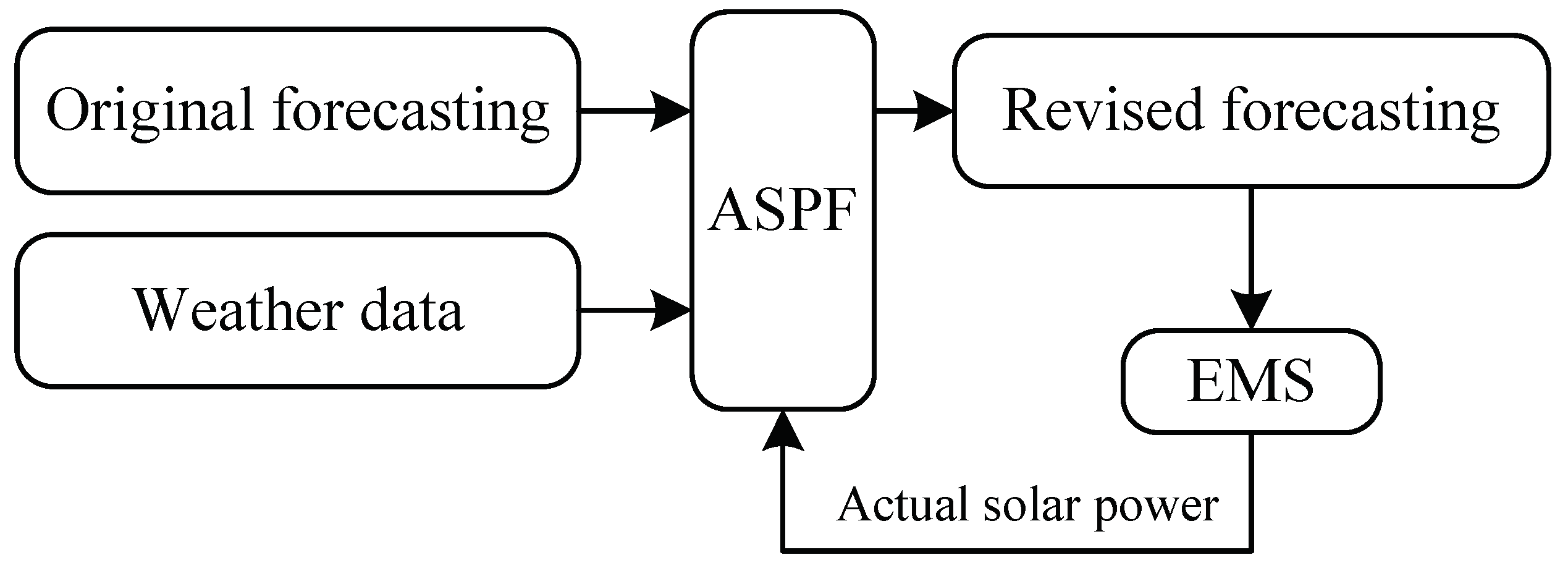
Therefore, an adaptive revising method on the original forecasting is highly desirable. Motivated by this, we propose an adaptive solar power forecasting (ASPF) method in this paper, which can revise the original forecastings adaptively according to the historical forecasting errors and the weather data. It combines data clustering, variable selection and artificial neural network (ANN) to achieve highly accurate revision on PV power predictions by learning the weather data and day-ahead forecasting errors intelligently and adaptively. The function of the ASPF is shown in Figure 1. Through ANN, ASPF learns the characteristics of forecasting errors between the predicted and actual PV power. By clustering the data, the capture of the forecasting characteristics could be highly improved. In addition, ASPF classifies the predicted day into similar day or non-similar (defined in Section 2), based on which the original forecastings are revised accordingly. The details are shown in Section 2. Also, ANN is adaptively upgraded so that ASPF improves as more data collected. Please note that ASPF actually captures the characteristics of forecasting errors and revises the predictions accordingly, and thus it does not require any specific original forecasting method, which can be a machine learning method or a statistical one. This makes ASPF a quite general method which can be used in many cases.
The remainder of this paper is organized as follows. We present the principle of ASPF and its framework in Section 2. The algorithms to realize ASPF are proposed in Section 3. The adaptive solar power forecasting is presented in Section 4. We perform the simulation studies in Section 5. Section 6 concludes this paper.
2. Principle and Framework of the ASPF
In this paper, the realization of ASPF mainly depends on the stored historical solar power data and the learning network which is updated according to the actual needs. In the database, we store the original predictive solar power , the revised solar power , and the actual solar power data . As more data collected, ASPF becomes more adaptive. Under certain condition, the historical solar power data are taken as the revised data directly, which is named as Similar Day Mode (SDM). On the other hand, when the condition of SDM does not hold, which is named as Non-similar Day Mode (NDM), ASPF modifies the original predictions by the output from a learning and updating network obtained from Back-propagation neural networks (BPNN) [25]. It learns the characteristics of differences between and . In this way, ASPF predicts more precisely for both SDM and NDM.
Furthermore, whatever the system is working in SDM or NDM, the network can be updated according to that whether the error between and is within an acceptable range or not. If the error is out of the allowed range, the network in ASPF is updated. We now present the mode judging standard, ASPF framework, and updating rules in this section. The notations used in this paper are summarized in Table 1.
2.1. Mode Judgment
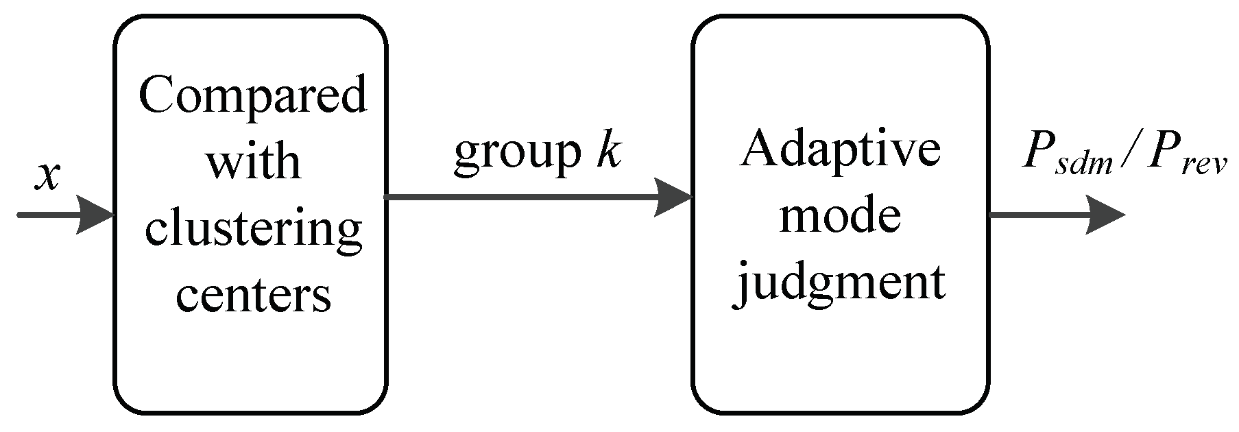
In order to quickly determine the similar days, K-means clustering [26,27] is used to divide the data into several groups firstly, and in every group, clustering center is adopted to judge whether there is a similar day in the current database rapidly, as shown in Figure 2. The input vector contains and key variables which affect the original predicting accuracy. x is then compared with clustering centers to be clustered into group k, if it has one or more similar days, and the closest historical solar power can be found in the database. Here, a variable denoted as is chosen as a threshold for the similar historical data, and if the error between x and is larger than , there is no similar day.
Considering the importance of clustering, we propose an improved k-means method to group the data, which is shown in Section 3.1. Please note that in different groups, the key weather variables may be different. For example, solar power is more closely related to temperature in sunny days than cloudy days. Therefore, we adopt a model-selection method called the least angular regression, also known as LARS [24], to analyze and find out the most correlated weather variables in different clusters.
The predicting network is thus acquired by combining the improved k-means clustering and LARS, which keeps updating for more accurate predictions. Besides, the trained BPNN, the weight w and the bias value b are used to determine the value of , which is thus closed related to the updated network. As the accuracy of the updated network increases, the similarity judgment is getting more precisely as well. We present the thorough steps to determine and update in Section 3 and Section 4.
2.2. Framework of the ASPF in SDM and NDM
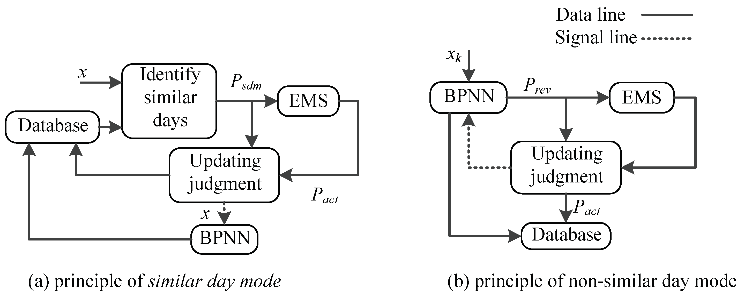
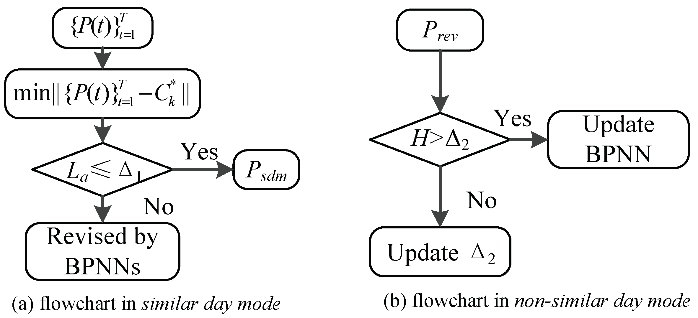
In order to show the principle of ASPF more clearly, we explain it from the following two aspects, namely, the operation of ASPF with similar days in SDM, and without similar day in NDM. The block diagrams are shown in Figure 3a,b, respectively.
Figure 3a shows the case when ASPF is working in SDM. x is compared with every data in group k until the closest data is found, which will be used as the revised PV power. Later, the actual solar power will be recorded in EMS when the whole day of operation ends. In order to testify the effectiveness of ASPF in SDM, and are compared in Updating judgment. If the largest difference between these two vectors at any time slot is less than a certain value, is chosen as , otherwise the network will be updated.
Figure 3b shows the case when ASPF is working in NDM. Because no similar day is found in the current database, ASPF learns the new data through BPNN and decides if the BPNN is updated or not. Different from SDM, is acquired by the BPNN, and the difference between and determines whether the network is updated in NDM. In this way, ASPF absorbs more useful data and thus becomes better in predictions.
2.3. Rules for Network Updating and Feedback
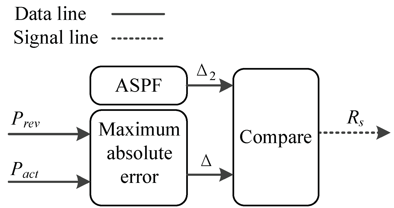
Figure 4 shows the rule of the Updating judgment function in Figure 3. is the day-ahead revised predictive PV power obtained from SDM or NDM, which is compared with , and is the maximum absolute error between and . represents acceptable error threshold between the revised solar power and the actual PV power in the current adaptive system. In addition, is updating as more data collected and processed, and will become smaller and smaller. It is also an indicator to measure the accuracy of predictions.
In the Updating judgment, if is larger then , a trigger signal is produced to activate BPNN. and BPNN is updated; otherwise, BPNN remains unchanged. Thus, the Updating judgment is mainly applied to renew the BPNN to guarantee accurate predictions. Here, is calculated by function Equations (9) and (17) in Section 3 and Section 4. We apply this both for SDM and NDM.
Through the above three parts, we compose the ASPF, and the complete realizations in every detail are presented next.
3. The Algorithms to Realize ASPF
This section presents the algorithms to realize ASPF. We first propose an improved k-means clustering method to divide the data into several groups. Then, LARS is presented to find the most relevant variables in every group. Followed by this, we discuss the compensation network for each group. We also present the feedback and updating mechanism.
3.1. Improved k-means Clustering
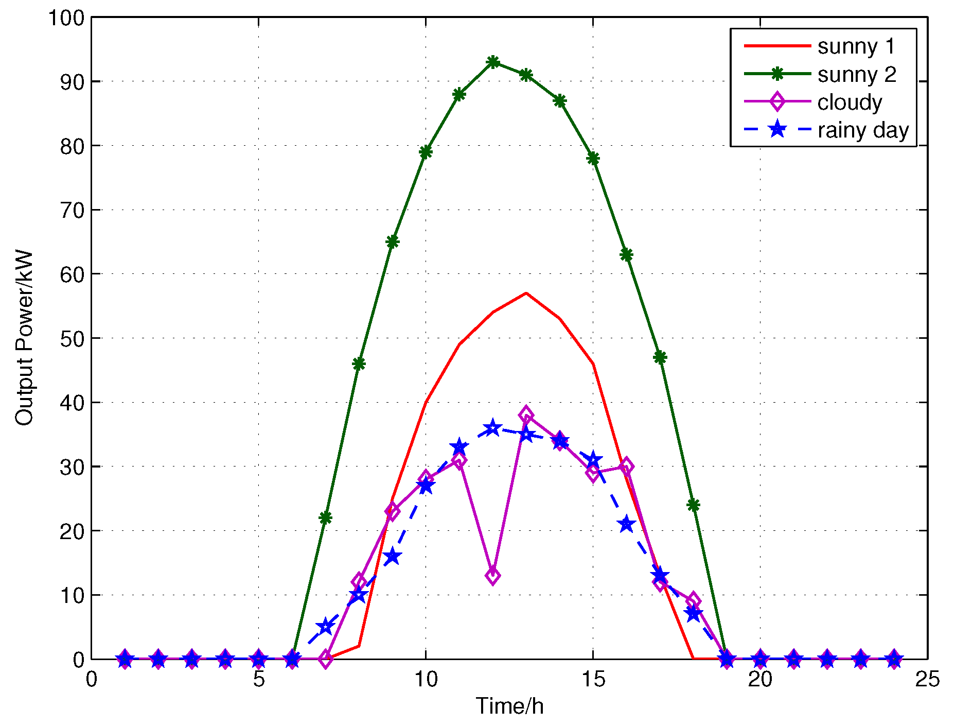
Figure 5 shows a typical daily solar power profile in different weather conditions, i.e., sunny, cloudy and rainy. sunny 1 and sunny 2 represent the sunny day in winter and summer, respectively. cloudy and rainy day’s solar power are different from the sunny days’. Therefore, considering the differences between these different weather types, we first cluster the data into several specific groups.
k-means is an effective, robust and widely used clustering technique [28]. It aims to cluster the data observations into K clusters, in which each observation belongs to the cluster with the nearest mean, and different clusters have low similarity with each other. It is implicitly assumed that features within a cluster are “homogeneous” and that different clusters are “heterogeneous” [26,29]. Here, we adopt k-means as a basis for clustering our data.
Given a dataset of N points and the number K of desired clusters, for each group, the corresponding generalized centroids are usually denoted as , and . The standard k-means finds the optimal cluster centers such that the sum of the 2-norm distance between each point , and the nearest cluster center is minimized [20,21]:
where is the coefficient which represents the degree of how the nth sample belongs to the kth cluster. For simplicity, in this paper. is changed from to during the calculation, and denotes the initial given clustering center for the group.
As mentioned in Section 1, the traditional k-means is sensitive to the initial center , and different initializations can lead to different final results. In recirculation iteration calculation, the k-means often converges to one or more clusters which contains very few or even no data point if the cluster center is given randomly.
To overcome this problem, we employ a simplified method which combines potential function and density function to get the initial cluster centers [21]. Firstly, for a given K, the density function of any sample is:
where is the function of effective radius of the neighborhood density, and the more data around sample , the greater is. , and is one constant. For a known sample set, the value of is easy to get. After the density of each data point has been computed, the data point with the highest density will be selected as the first cluster center , and is the density value. Then, the density function in the subsequent cluster becomes:
where , and , so the remaining cluster centers can be identified as according . Based on this result, the function Equation (1) will be convergent through few iterations, and no initial clustering will be empty.
k-means consists of two phases: one for determining the initial centroids and the other for assigning data points to the nearest clusters and then recalculating the cluster means. The second phase is necessary for finding the optimal k, and the data within the same type are very similar, while the data from different types are not close.
In this paper, the method discussed in [30] is adopted to obtain optimal number of k. Here, an inner distance in the same group is defined as:
where is the average distance from data in cluster k to other data in the same group, and denotes the number of data in the cluster, . If is small, the data in this cluster is also compact correspondingly.
The distance for data between different groups is defined as:
where represents the minimal average distance of the data from cluster k to other clusters. In addition, the larger value of the is, the feature of “heterogeneous” is more clear. In order to synthesize the two factors, and , the linear combination is used to balance the relationship between them. At the same time, in order to enable the indicator to analyze the validity of the data clustering and to avoid the index from being affected by the dimension, the fractional operation is employed. The index to calculate the optimal k is defined as:
where . Since the requires at least two clusters, k starts from 2 to K. From Equation (6), it can be seen that when the cluster number k is taken from 2 to K, the optimal k is confirmed if the gets the maximal value. Usually, , [31].
Eventually, based on the condition of getting a suitable initial cluster centers and the optimal number of k, pseudo-code for the improved k-means clustering is summarized in Algorithm 1.
| Algorithm 1: Improved k-means Algorithm |
| Step 1: For each , . |
| Step 2: In each cluster k, the initial cluster center is obtained by executing Equations (2) and (3), then & can be calculated by Equation (1). |
| Step 3: Find and record based on Equations (4)–(6). Compare k with K, and if , and repeat Step 2; otherwise, jump to Step 4. |
| Step 4: Acquire the maximal and the corresponding number , recalculate Equations (2) and (3), then the optimal clustering data is obtained through Equation (1), and the optimal centers are , weather types are , . |
In this way, solar power data is divided into several groups by the proposed improved k-means clustering. According to the standardized-residual method and Lagrange Interpolation Polynomial [32], the abnormal data is removed and the remaining data are normalized.
3.2. The Least Angular Regression Algorithm
A typical regression can be expressed as: , where is the current estimate of the vector of responses with M predictors, is one matrix with , N is the number of sample, and then current correlation will be: , and there will exist a j such that is maximized. Then will be updated by rule of , in LARS, is endogenously chosen so that the algorithm proceeds equiangular between the variables in the most correlated set (hence the ‘least angle direction’) until the next variable is found. Then the next variable joints the active set, and their coefficient are moved together in a way that keeps their correlations tied and decreasing. This process is continued until all the variables in the model, and end at the full least-squares fit [24].
Actually, the LARS algorithm begins at , supposing is current estimate and let . Define as a subset of the indices corresponding to variable with largest absolute correlations, and . Defining , and active matrix corresponding to is . Letting and , is a vector of s of length equaling , the size of . Then the equiangular vector can be defined as , where , is the unit vector making equal angles, less than , with the columns of which satisfies , and , and . Then the will be updated in the next step of the LARS algorithm is:
where
indicates that the minimum is taken over only positive components within each choice of m, . Finally, dependency variables are sorted by relevance level, and we can easily get the important predictors by LARS.
After the dataset is divided in several styles in Section 3.1, and these subsets are defined as , respectively. Then each subset is analyzed by LARS to reduce the influence of uninformative predictors, and we can focus on variables which is significant for the differences in prediction.
3.3. BPNN-Based Solar Power Compensation
The BPNN, one of the most popular techniques in the filed of neural network, is a kind of supervised learning NN. It uses the steepest gradient descent method to reach very small approximation. Theoretically, BPNN can approximate any nonlinear functions [25], in fact, for the PV power prediction, the relationship between its input data and forecasting value is very complicated [8]. So it is suitable to adopt the BPNN in our ASPF to learn this feature. Therefore, a three-layered feed-forward neural network and the BP learning algorithm are adopted together to compensate the predictive error of solar power in this paper.
The input nodes of the BPNN to the hidden layer is decided by the result from Section 3.2, x consists of the from to T. B denotes the number of the input nodes, and is the kth group of inputing predictive message at time slot t. For the number of hidden neurons (HN) in the hidden layer, the method in [33] is used to get the upper bound on the number of hidden neurons, HN. Then the hidden neurons h is ranged from 1 to HN, and the model is trained for several times according the method in [34], and the forecasting mean square error from the testing data is calculated and recorded for comparisons. The optimal is acquired in the end, which is the number occuring mostly in the iteration with the less mean square error.
Initializing the weight is another important step in BPNN, and initialization of a network involves assigning initial values for the weights of all connecting links, here, initial values for the weights are set in the small random values between and [33]. Momentum coefficient and learning rate in BPNN are chosen from and , respectively. Besides, in order to overcome the possible overfitting problem in forecasting, regularization is employed of the parameter ranged in for groups of models.
Finally, Maximum Absolute Error (MxAE), Root Mean Squared Error (RMSE) and Mean Absolute Percentage Error (MAPE) between the revised solar power and the actual value are used to quantify the performance of each group. MxAE, RMSE and MAPE are widely used statistical measurements of the accuracy of the models [22]. In addition, in each group, MxAE, RMSE and MAPE are defined as follows:
where is the number of predicted points in type k, is actual solar power for the nth point, and represents the revised solar power.
3.4. Closed-Loop Feedbacks and Updates
ASPF not only has the ability to compensate the error existed in original predictive solar power day-ahead, but also uses the historical solar actual power as the revised value. So, it is necessary to search for a similar day in the system. Besides, it should be feasible to use as a substitute of , and important to guarantee this with high accuracy. All above requirements are accomplished by the closed-loop feedback and updating mechanism.
In this paper, we use to define the MxAE of the current forecasting model. In addition, the criteria for judging similar days is related to network parameters and determined by the maximal absolute error of the current BPNN. with the input data of , BPNN can get the difference of the predictive PV power and the actual values, if this difference is less than , their corresponding actual values will be replaced by each other with acceptable errors. So the actual solar power of the similar data can be used as the revised value directly when this similarity meets certain conditions. Here, the specific relationship of the with the BPNN and this condition are shown below.
The original forecasting models are built in Section 3.3, and after the models are trained, MxAE, weight and bias b can be obtained from BPNN. BPNN can be formulated as the non-linear function, expressed as:
and for any input data , if it satisfies:
and the function has the properties of monotonically increasing and derivable. So .
In case 1, if , the actual solar power will be larger than the revised one. Thus,
so,
In case 2, if , the relationship of Equation (15) also can be obtained.
Therefore, with the difference obtained by input data , is known, if the result of is less then , and will be replaced by each other with acceptable errors. On the other hand, when the prediction model is invariant, by comparing the similarity of predicted input information, the actual solar power of similar historical day can be used as the revised PV power directly if it satisfies certain condition. In addition, we give this condition below.
In practice, through comparing the maximal and the corresponding value calculated by the is known, it can be found that if , then . So the initial can be chosen as , and thus has a close relationship with the updated network. As the accuracy of the updating network increases, the precision of the similar days’ solar power prediction becomes higher and higher. So it is reasonable to adopt historical actual solar power as the day-ahead revised data when the similar input message exists. Our proposed method is available for reusing the historical data to achieve better forecasting revision.
4. Adaptive Solar Power Forecasting Algorithm
Based on the Algorithms in Section 3, in this section, we present the complete ASPF.
4.1. Effectiveness of the ASPF
As more data collected, there will be more and more historical data in database, so it is not proper to use an invariant parameter as to search for the similar day. Meanwhile, the potential function in [21] has a good performance of slow decaying. Based on this, the decaying of is defined as:
where is current value, represents the updated value of in the presence of multiple similar days, , and , . In Equation (16), is updated only when more than two similar days exist. The flow chart in SDM is shown in Figure 6a.
Similarly, the forecasting error gradually decreases with the increasing amount of the testing data. In addition to this, in the system, the networks can be re-trained when the predictive error beyond the . Meanwhile, if MxAE of the testing day is less than the initial , it is then to decrease , obtained from Equation (9), where d represents the index of the day. The decreasing of follows
where is the updated value of . The flow chart of updating BPNN and is shown in Figure 6b.
Figure 7 shows the complete flow chart of ASPF, in which the forecasting accuracy can be improved gradually, and the historical data is thus used more effectively. Moreover, according to the similar daily information, ASPF adaptively identifies and compensates for the predicted solar power day-ahead.
4.2. The Algorithm of whole System
Based on the above analysis, we now summarize the complete steps of the algorithm to realize the ASPF in Algorithm 2.
| Algorithm 2: Adaptive Solar Power Forecasting Algorithm |
| Step 1: The historical data is divided into different groups by Algorithm 1, and corresponding clustering centers are confirmed. |
| Step 2: LARS is used to each group to get its important predictors, and BPNN is employed to learn the features in every group, subsequently, according the principle in Section 3.4, and is setup. |
| Step 3: For a new and its important predictors, compares with , if the maximal error is less than , go to Step 4; otherwise, go to Step 5. |
| Step 4: and its important predictors compares with every data in group k, and finds the most similar day as , and update according formulation Equation (16), then go to Step 6. |
| Step 5: is revised by BPNN, and the day-ahead PV power is obtained, go to Step 6. |
| Step 6: , if any element in is larger than , update the BPNN, storage and in EMS, then go to Step 3; otherwise, go to Step 7. |
| Step 7: According to formulation Equation (17) update , and go to Step 3. |
5. Simulation Results
In this section, we test the performance of ASPF based on the trace obtained from a small power system in China. In order to validate the proposed algorithm, we apply it in the original forecasting PV power which is predicted by radial basis function NN and Multiple Linear Regression (MLR). The algorithms including the improved k-means, LARS, BPNN and ASPF are verified via simulations and comparisons.
5.1. Data Description
In this paper, the small power system consists of micro-diesel, photovoltaic array, lithium battery cabinet and load demand. The simulations are performed to verify the operation of the proposed algorithm. The data used in ASPF comes from the actual factory which locates in Hekou town, Nantong city, China(). For PV power forecasting, the prediction can be performed every 2 h, 1 h, 0.5 h, or 15 min according to users’ demand. All the simulations complete in the MATLAB, and in our ASPF the computation time mainly depends on the BPNN which only takes several seconds one time in Matlab. So the results of ASPF can be used in day-ahead energy management, and it can be applied to the real-time energy management too. In this paper, the parameter for the PV power adaptive compensation time interval is set to 1 h based on our system. In this system, solar power is mainly supplied to the canteen and the water pumps in the factory. According to the historical data, we obtain the original forecasting PV power in NN and MLR respectively, and store them in EMS.
5.2. Predicting Compensation of ASPF
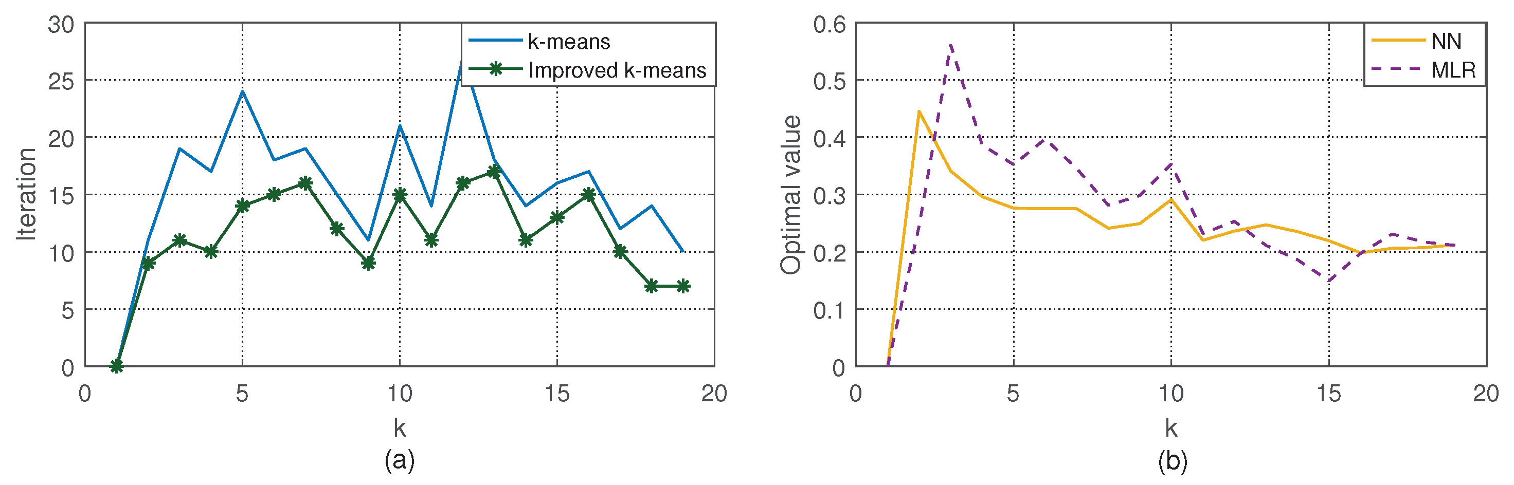
The data of original solar power is from 1 January to 31 December 2016 in Hekou town. For the k-means algorithm, the initial cluster centers calculated by the potential function need less iterations compared with traditional stochastic way, as shown in Figure 8a. As explained in Section 3.1, the range of k is from 2 to 19. In addition, the initial cluster centers can be found fast and better to determine the optimal number of clusters, and effectively avoid the occurrence of non-clustering situation. Equations (4)–(6) are used to determine the optimal number of clusters. Based on the methods described in Section 3.1, the number of clusters for different k under NN and MLR are shown in Figure 8b, where we can see that the optimal number of clusters is in NN, and in MLR.
In order to modify the differences in original method for forecasting day-ahead solar power, LARS is used to analyze the key factors which affect the forecasting most in NN and MLR. In addition, the critical parameters are different in NN and MLR, shown in Table 2 and Table 3. The forecasting results of NN and MLR for different groups are summarized in Table 4 and Table 5, which show that our proposed method has greatly improved the accuracy of PV prediction no matter the PV power is predicted by machine learning or MLR.
5.3. Performance Evaluation of ASPF
We now validate that our ASPF can adaptively revise the solar power which is predicted by NN. We randomly select 100 days of data from 1 January to 31 October 2016, and store the data as the initial database, which includes both predictive information and PV actual power. The data in the database gradually accumulates as the number of days increases in this system. Data from 1 November to 30 December 2016 are used to test the effectiveness of the ASPF. By comparing with the cluster centers and , 1 has 23 data points, and 2 has 37. Here, , .
For these 60 testing days, the ASPF results are in Table 6. NL is the number of days whose MxAE is smaller than , and NB denotes the number of days whose MxAE is larger than . Through Table 6, it can be observed that there are 8 times with similar day, and 15 times with no similar day in 1. Due to the stored data in 1 is less than in 2, there are only 4 times that the historical actual value can be accepted as revised solar power. The non-similar day data are revised by our proposed BPNN, and the results are ideal as their MxAEs are less than . Moreover, the similar day number of group 2 is more than that in group 1 because there are more data in 2 in the database. There is also one non-similar day’s result predicted by BPNN over the , because the weather changes are more complex in non-sunny circumstances which lead to larger errors. However, the overall performance of our proposed methods is very stable and reliable.
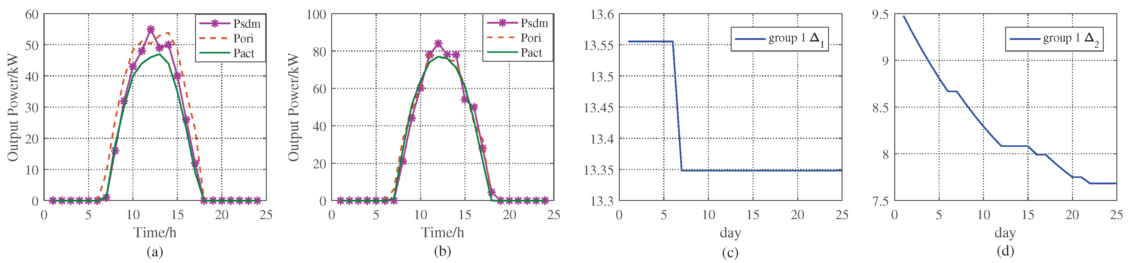
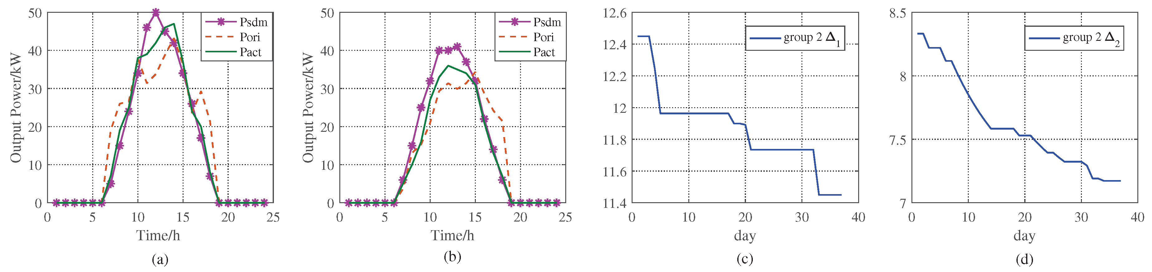
The comparisons between the proposed method and the historical data are shown in Figure 9 and Figure 10. Here, denotes the corresponding historical actual solar power if similar days exist. is the predicted solar power by original method. represents the actual solar power of the day. Figure 9a shows the result when there is a similar day in 1 and when , is used as the revised PV power. In addition, at the night of the day, we can know the actual solar power by EMS, the MxAE between the and will be gotten, here MxAE is 9.112, less than initial , which is 9.476. In Figure 9b, there are 3 similar days, and the actual MxAE between and is 8.351, larger than the current . In Figure 9d, the data of the 13rd day are used to retrain the BP neural network. When , there is no similar day, so BPNN is used to get the day-ahead revised solar power as shown in Table 7. And the MxAEs in these days are less than 9.476, so gradually reduces. does not update when BPNN is not working as shown in Figure 9d for the 6th and the 7th day. Figure 9c illustrates the in EMS, and if there is no similar day or the number of similar days is 1, is constant. When the number of similar days is larger than 1, it means several similar days are in the database, and should be lowered in order to find possible similar days as the data increases. In this way, the efficiency of ASPF keeps improving. Please note that, we plot the results for sunny day in Figure 9 and Figure 10, however, our simulation results are not only effective for sunny days, but also for PV power revision in other weather types, such as cloudy, rainy day. It can be seen in Table 7 and Table 8, because the data in 1 or 2 can be any weather types.
The results from 2 are shown in Figure 10. The number of similar days increase, the change in and are even more apparent than 1. This change depends on the number of operation days. Table 7 and Table 8 record the detailed steps in 1 and 2. Here, SI is an indicator of the existence of similar days: 1 indicates similar days exist, while 0 means no similar day. TS represents the number of similar days when SI . WD is the MxAE in , and is less than . In contrast, BD indicates that the MxAE is greater than . NS is the opposite of SI, and NS = 1 means no similar day. and are used to record the states of our revised prediction performance after updating.
In Table 7, BD is 1 in the 13th day, which means the similar day’s actual value has a large deviation from the 13th day’s actual solar power. In addition, then, ASPF retrains the network using the 13th day’s data at the end of the 13th day. When there is similar day close to the 13th day at the 18th day, the 13th day’s actual solar power is adopted as day-ahead revised power and the MxAE is less than . The same situation also happens in 2, as shown in Table 8. In 2, at the 3rd day, there is no similar day, solar power is revised by BPNN and then stored in database as shown in Table 8. In addition, the 25th day is similar to the 3rd day’s information, so the 3rd day’s actual solar power is used as the 25th day’s revised power, and the result is acceptable as shown in Figure 10d. This reveals that as the number of data increases, the results of adopting similar day’s actual power become more accurate, and the predictive input message can be identified and compensated adaptively.
Through the above simulations, it is reasonable to use the similar day’s actual value as the solar forecast power if the forecasting data satisfies the certain condition, which limits the deviation of the predicted data be less than . Also, because BPNN updates the network when MxAE exceeds , this also ensures that BPNN can effectively predict the data in different situations. In the case of 98%, BPNN can get satisfactory results in this system.
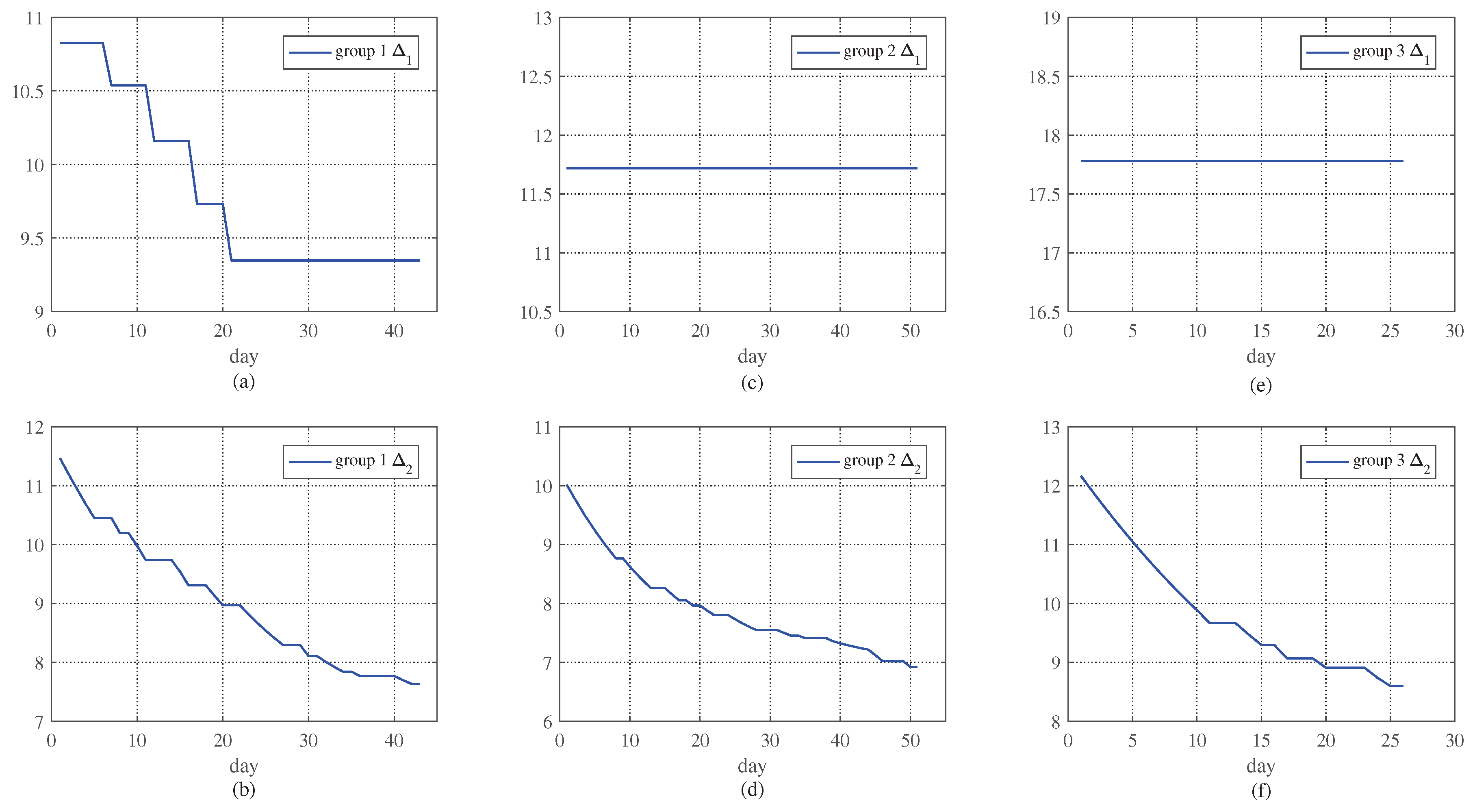
Furthermore, in order to verify the wide applicability of our proposed ASPF algorithm, we run similar simulation for the PV power predicted by MLR, and compare the result. Firstly, 150 days data from 1 January 2016 to 31 August 2016 are randomly selected as the initial database to get the MLR predictive PV power. Then, we select 120 days from 1 September, to 31 December 2016 as testing data. According to the results of k-means, the data of the testing days is classified into three groups, which contain 43, 51, and 26 days, respectively. In addition, the ASPF simulation results are shown in Figure 11. In Figure 11a, gradually decreases as the number of days increases, because the data in 1 has more accurate predictions than 2 from Table 5. As decreases in Figure 11b, the network updates continuously, and the number of similar days increases so that becomes smaller correspondingly. For Figure 11c,e, does not change, because in 2 and 3, the number of the similar days are less than in 1. in Figure 11d,f decrease gradually, and thus the accuracy of our method improves continuously. In summary, the proposed ASPF obtains high-precision prediction values in both non-similar days and similar day mode under different predicting methods.
6. Conclusions
In this paper, we propose an adaptive solar power forecasting algorithm for highly precise solar power forecasting. We firstly present the adaptive framework of the algorithm, integrating the improved k-means clustering, LARS and BPNN. ASPF is thus able to select the important variables, compensate the predictions from different methods, and update the BPNN adaptively. We also present these algorithms in details. Finally, we evaluate the proposed ASPF through the simulated experiments. We verify the validity of these algorithms, such as, improved k-means, LARS, BPNN and ASPF. Furthermore, we testify the effectiveness of the ASPF algorithm for different prediction models. The simulation results show that our proposed method greatly improves the accuracy of solar power, and keeps improving as more data collected. For future work, we consider to apply ASPF in other application, such as energy scheduling mentioned in Introduction.
Author Contributions
Y.W. proposed the conceptualization of adaptive forecasting the solar power; Y.W., H.Z., F.Z. and J.C. worked together to investigate the proper method to realize this adaptive solar power forecasting; H.Z., X.C. and F.Z. validated the performance in Matlab, and the test data is provided by X.C.; H.Z. and Y.W. analyzed the data and wrote the paper; X.C., F.Z. and J.C. supervised the all the entire process.
Funding
The authors gratefully acknowledge financial support for this project provided by the NSF of China under Grants No. 51607087 and the Fundamental Research Funds for the Central Universities of China, NO. XCA17003-06.
Conflicts of Interest
The authors declare no conflict of interest.
References
- Wang, Y.; Mao, S.; Nelms, R.M. Online Algorithms for Optimal Energy Distribution in Microgrids; Springer International Publishing: Berline, Germany, 2015. [Google Scholar]
- Wang, Y.; Mao, S.; Nelms, R.M. On Hierarchical Power Scheduling for the Macrogrid and Cooperative Microgrids. IEEE Trans. Ind. Inform. 2015, 11, 1574–1584. [Google Scholar] [CrossRef]
- Liang, H.; Zhuang, W. Stochastic Modeling and Optimization in a Microgrid: A Survey. Energies 2014, 7, 2027–2050. [Google Scholar] [CrossRef]
- Meng, L.; Sanseverino, E.R.; Luna, A.; Dragicevic, T.; Vasquez, J.C.; Guerrero, J.M. Microgrid supervisory controllers and energy management systems: A literature review. Renew. Sustain. Energy Rev. 2016, 60, 1263–1273. [Google Scholar] [CrossRef]
- Wang, Y.; Mao, S.; Nelms, R.M. Online Algorithm for Optimal Real-Time Energy Distribution in the Smart Grid. IEEE Trans. Emerg. Top. Comput. 2013, 1, 10–21. [Google Scholar] [CrossRef]
- Wang, Y.; Shen, Y.; Mao, S.; Cao, G.; Nelms, R.M. Adaptive Learning Hybrid Model for Solar Intensity Forecasting. IEEE Trans. Ind. Inform. 2018, 14, 1635–1645. [Google Scholar] [CrossRef]
- Soman, S.S.; Zareipour, H.; Malik, O.; Mandal, P. A review of wind power and wind speed forecasting methods with different time horizons. In Proceedings of the North American Power Symposium, Arlington, TX, USA, 26–28 September 2010; pp. 1–8. [Google Scholar]
- Antonanzas, J.; Osorio, N.; Escobar, R.; Urraca, R.; Martinez-De-Pison, F.J.; Antonanzas-Torres, F. Review of photovoltaic power forecasting. Solar. Energy 2016, 136, 78–111. [Google Scholar] [CrossRef]
- Bacher, P.; Madsen, H.; Nielsen, H.A. Online short-term solar power forecasting. Solar. Energy 2009, 83, 1772–1783. [Google Scholar] [CrossRef] [Green Version]
- Liu, J.; Fang, W.; Zhang, X.; Yang, C. An Improved Photovoltaic Power Forecasting Model with the Assistance of Aerosol Index Data. IEEE Trans. Sustain. Energy 2015, 6, 434–442. [Google Scholar] [CrossRef]
- Shi, J.; Lee, W.J.; Liu, Y.; Yang, Y.; Wang, P. Forecasting Power Output of Photovoltaic Systems Based on Weather Classification and Support Vector Machines. IEEE Trans. Ind. Appl. 2015, 48, 1064–1069. [Google Scholar] [CrossRef]
- Su, W.; Wang, J.; Roh, J. Stochastic Energy Scheduling in Microgrids with Intermittent Renewable Energy Resources. IEEE Trans. Smart Grid 2014, 5, 1876–1883. [Google Scholar] [CrossRef]
- Osório, G.J.; Lujano-Rojas, J.M.; Matias, J.C.O.; Catalão, J.P.S. Including forecasting error of renewable generation on the optimal load dispatch. In Proceedings of the 2015 IEEE Eindhoven PowerTech, Eindhoven, The Netherlands, 29 June–2 July 2015; pp. 1–6. [Google Scholar]
- Palma-Behnke, R.; Benavides, C.; Lanas, F.; Severino, B.; Reyes, L.; Llanos, J.; Sáez, D. A Microgrid Energy Management System Based on the Rolling Horizon Strategy. IEEE Trans. Smart Grid 2013, 4, 996–1006. [Google Scholar] [CrossRef]
- Chen, C.; Duan, S.; Cai, T.; Liu, B. Smart energy management system for optimal microgrid economic operation. Renew. Power Gener. Iet 2011, 5, 258–267. [Google Scholar] [CrossRef]
- Ding, M.; Wang, L.; Bi, R. An ANN-based Approach for Forecasting the Power Output of Photovoltaic System. Proc. Environ. Sci. 2011, 11, 1308–1315. [Google Scholar] [CrossRef]
- Yesilbudak, M.; Çolak, M.; Bayindir, R. A review of data mining and solar power prediction. In Proceedings of the IEEE International Conference on Renewable Energy Research and Applications, Birmingham, UK, 20–23 November 2016; pp. 1117–1121. [Google Scholar]
- Benmouiza, K.; Cheknane, A. Forecasting hourly global solar radiation using hybrid k-means and nonlinear autoregressive neural network models. Energy Convers. Manag. 2013, 75, 561–569. [Google Scholar] [CrossRef]
- Mccandless, T.C.; Haupt, S.E.; Young, G.S. A regime-dependent artificial neural network technique for short-range solar irradiance forecasting. Renew. Energy 2016, 89, 351–359. [Google Scholar] [CrossRef] [Green Version]
- Huang, X.; Ye, Y.; Zhang, H. Extensions of Kmeans-Type Algorithms: A New Clustering Framework by Integrating Intracluster Compactness and Intercluster Separation. IEEE Trans. Neural Netw. Learn. Syst. 2014, 25, 1433–1446. [Google Scholar] [CrossRef] [PubMed]
- Chiu, S.L. Fuzzy model identification based on cluster estimation. J. Intell. Fuzzy Syst. 1994, 2, 267–278. (In Chinese) [Google Scholar]
- Tang, N.; Mao, S.; Wang, Y.; Nelms, R.M. Solar Power Generation Forecasting with a LASSO-Based Approach. IEEE Int. Things J. 2018, 5, 1090–1099. [Google Scholar] [CrossRef]
- Hastie, T.; Tibshirani, R.; Friedman, J. The Elements of Statistical Learning: Data Mining, Inference, and Prediction; Springer: Berline, Germany, 2001. [Google Scholar]
- Efron, B.; Hastie, T.; Johnstone, I.; Tibshirani, R. Least angle regression. Ann. Stat. 2004, 32, 407–451. [Google Scholar]
- Rumelhart, D.E.; Hinton, G.E.; Williams, R.J. Learning representations by back-propagating errors. Nature 1986, 323, 399–421. [Google Scholar] [CrossRef]
- Hartigan, J.A.; Wong, M.A. Algorithm AS 136: A K-Means Clustering Algorithm. J. Roy. Stat. Soc. 1979, 28, 100–108. [Google Scholar] [CrossRef]
- Kanungo, T.; Mount, D.M.; Netanyahu, N.S.; Piatko, C.D.; Silverman, R.; Wu, A.Y. An efficient k-means clustering algorithm: analysis and implementation. IEEE Trans. Pattern Anal. Mach. Intell. 2002, 24, 881–892. [Google Scholar] [CrossRef]
- Ratanamahatana, C.A.; Lin, J.; Gunopulos, D.; Keogh, E.; Vlachos, M.; Das, G. Mining Time Series Data. Data Min. Knowl. Discov. Handb. 2005, 1069–1103. [Google Scholar]
- Modha, D.S.; Spangler, W.S. Feature Weighting in k-Means Clustering. Mach. Learn. 2003, 52, 217–237. [Google Scholar] [CrossRef]
- Zhou, S.B.; Xu, Z.Y.; Tang, X.Q. Method for determining optimal number of clusters in K-means clustering algorithm. J. Comput. Appl. 2010, 30, 1995–1998. [Google Scholar] [CrossRef]
- Rezaee, M.R.; Lelieveldt, B.P.F.; Reiber, J.H.C. A new cluster validity index for the fuzzy c-mean. Pattern Recognit. Lett. 1998, 19, 237–246. [Google Scholar] [CrossRef]
- Liu, L.; Zhai, D.; Jiang, X. Current situation and development of the methods on bad-data detection and identification of power system. Power Syst. Prot. Control 2010, 38, 143–147. [Google Scholar]
- Govindaraju, R.S.; Rao, A.R. Artificial Neural Networks in Hydrology. J. Hydrol. Eng. 2000, 5, 124–137. [Google Scholar]
- Jiao, B.; Ye, M. Determination of Hidden Unit Number in a BP NeuraI Network. J. Shanghai Dianji Univ. 2013, 16, 113–116, 124. (In Chinese) [Google Scholar]
Figure 1.
The function of ASPF.

Figure 2.
The principle of the Identify similar days.

Figure 3.
The ASPF schematic in different mode.

Figure 4.
The principle of Updating judgment.

Figure 5.
The solar power for different weather types.

Figure 6.
The flow chart for searching similar days.

Figure 7.
The flow chart for ASPF in power systems.

Figure 8.
(a) The iterations in traditional and improved k-means. (b) The curve of determining the optimal number of clusters.
Figure 8.
(a) The iterations in traditional and improved k-means. (b) The curve of determining the optimal number of clusters.

Figure 9.
The results of 1 in ASPF. (a) denotes that there is a similar day, and the MxAE between the actual solar power and historical value is less than ; on the contrary, (b) shows the results that the MxAE is larger than ; (c) plots a curve that the in 1 changes with the similar days’ message; (d) shows the in 1 changing with MxAE.

Figure 10.
The results of 2 in ASPF. (a) denotes that there is a similar day, and the MxAE between the actual solar power and historical value is less than ; on the contrary, (b) shows that the MxAE is larger than ; (c) plots a curve that the in 2 changes with the similar days’ message; (d) shows the in 2 changing with MxAE.

Figure 11.
The results of ASPF applied to compensate the solar PV predicted by MLR. (a,c,e) are the trend of in 1, 2 and 3. (b,d,f) denote the in 1, 2 and 3 respectively.
Figure 11.
The results of ASPF applied to compensate the solar PV predicted by MLR. (a,c,e) are the trend of in 1, 2 and 3. (b,d,f) denote the in 1, 2 and 3 respectively.


Table 1.
Notation.
| Symbol | Description | Symbol | Description |
|---|---|---|---|
| the original predictive solar power | initial given clustering center in group k | ||
| the revised solar power | optimal clustering center in group k | ||
| the actual solar power | density function value of the nth data in order to calculate the initial center of th cluster | ||
| the historical solar power | the kth group initial cluster center | ||
| the threshold to judge the similar day | inner distance in the same group | ||
| the updated value of | the minimum distance between different groups | ||
| acceptable error between and | intra-group and inter-group index | ||
| the updated value of | the number of data in kth cluster | ||
| signal to trigger the network updating | the gth data in group k | ||
| x | the vector contains and weather data | correlation coefficient of residual | |
| N | the total number of x | the predictive value of the nth data | |
| k | clustering number | w | the weight of neural network |
| K | the maximum number of clusterings | b | the bias value of neural network |
| the kth clustering center | h | the number of hidden neurons | |
| total number of similar days or non-similar day | the number of days with the MxAE less than | ||
| the number of days with the MxAE larger than | the indicator to record whether there is a similar day | ||
| the number of similar days when in and | the indicator to record whether MxAE in and | ||
| the indicator to record whether MxAE | the indicator to record state after NN updated | ||
| the indicator to record state after NN updated | the indicator without similar day |
Table 2.
The results of variable selection by LARS in NN.
| Pattern | Key Factors | ||
|---|---|---|---|
| group 1 | Original solar power | Air temperature | |
| group 2 | Original solar power | Air temperature | Sunshine duration |
Table 3.
The results of variable selection by LARS in MLR.
| Pattern | Key Factors | |||
|---|---|---|---|---|
| group 1 | original PV power | Sunshine duration | Air temperature | Relative humidity |
| group 2 | original PV power | Relative humidity | Air temperature | Sunshine duration |
| group 3 | original PV power | Air temperature | Sunshine duration |
Table 4.
Comparison of forecasting results in NN.
| RMSE (kW) | MAPE (%) | MxAE (kW) | |
|---|---|---|---|
| group 1 | 3.66 | 4.30 | 9.476 |
| 9.31 | 16.42 | 22.34 | |
| group 2 | 1.74 | 7.04 | 8.33 |
| 6.44 | 31.91 | 18.14 |
Table 5.
Comparison of forecasting results in MLR.
| RMSE (kW) | MAPE (%) | MxAE (kW) | |
|---|---|---|---|
| group 1 | 3.02 | 7.43 | 10.01 |
| 9.01 | 51.04 | 25.51 | |
| group 2 | 3.87 | 8.39 | 9.67 |
| 9.59 | 44.73 | 20.46 | |
| group 3 | 2.68 | 6.54 | 8.54 |
| 11.99 | 34.66 | 23.14 |
Table 6.
The results of ASPF.
| Pattern | Similar Days | Non-Similar Day | ||||
|---|---|---|---|---|---|---|
| NT | NL | NB | NT | NL | NB | |
| 1 | 8 | 4 | 4 | 15 | 15 | 0 |
| 2 | 17 | 12 | 5 | 20 | 19 | 1 |
Table 7.
The results of ASPF in 1.
| Day | 1 | 2 | 3 | 4 | 5 | 6 | 7 | 8 | 9 | 10 | 11 | 12 | 13 | 14 | 15 | 16 | 17 | 18 | 19 | 20 | 21 | 22 | 23 |
|---|---|---|---|---|---|---|---|---|---|---|---|---|---|---|---|---|---|---|---|---|---|---|---|
| SI | 1 | 0 | 0 | 0 | 0 | 0 | 1 | 0 | 0 | 0 | 0 | 0 | 1 | 1 | 1 | 0 | 1 | 1 | 0 | 0 | 1 | 0 | 0 |
| TS | 1 | 0 | 0 | 0 | 0 | 0 | 3 | 0 | 0 | 0 | 0 | 0 | 1 | 1 | 1 | 0 | 1 | 1 | 0 | 0 | 1 | 0 | 0 |
| WD | 1 | 0 | 0 | 0 | 0 | 0 | 1 | 0 | 0 | 0 | 0 | 0 | 0 | 1 | 0 | 0 | 0 | 1 | 0 | 0 | 0 | 0 | 0 |
| BD | 0 | 0 | 0 | 0 | 0 | 0 | 0 | 0 | 0 | 0 | 0 | 0 | 1 | 0 | 1 | 0 | 1 | 0 | 0 | 0 | 1 | 0 | 0 |
| NS | 0 | 1 | 1 | 1 | 1 | 1 | 0 | 1 | 1 | 1 | 1 | 1 | 0 | 0 | 0 | 1 | 0 | 0 | 1 | 1 | 0 | 1 | 1 |
| 0 | 1 | 1 | 1 | 1 | 1 | 0 | 1 | 1 | 1 | 1 | 1 | 0 | 0 | 0 | 1 | 0 | 0 | 1 | 1 | 0 | 1 | 1 | |
| 0 | 0 | 0 | 0 | 0 | 0 | 0 | 0 | 0 | 0 | 0 | 0 | 0 | 0 | 0 | 0 | 0 | 0 | 0 | 0 | 0 | 0 | 0 |
Table 8.
The results of ASPF in 2.
| Day | 1 | 2 | 3 | 4 | 5 | 6 | 7 | 8 | 9 | 10 | 11 | 12 | 13 | 14 | 15 | 16 | 17 | 18 | 19 | 20 | 21 | 22 | 23 | 24 | 25 | 26 | 27 | 28 | 29 | 30 | 31 | 32 | 33 | 34 | 35 | 36 | 37 |
|---|---|---|---|---|---|---|---|---|---|---|---|---|---|---|---|---|---|---|---|---|---|---|---|---|---|---|---|---|---|---|---|---|---|---|---|---|---|
| SI | 1 | 1 | 0 | 1 | 1 | 0 | 1 | 0 | 0 | 0 | 0 | 0 | 0 | 0 | 1 | 1 | 1 | 1 | 0 | 1 | 1 | 0 | 0 | 0 | 1 | 0 | 0 | 1 | 1 | 1 | 0 | 0 | 1 | 0 | 0 | 1 | 0 |
| TS | 1 | 2 | 0 | 5 | 5 | 0 | 1 | 0 | 0 | 0 | 0 | 0 | 0 | 0 | 2 | 1 | 1 | 2 | 0 | 2 | 5 | 0 | 0 | 0 | 1 | 0 | 0 | 1 | 1 | 1 | 0 | 0 | 1 | 0 | 0 | 7 | 0 |
| WD | 1 | 0 | 0 | 1 | 1 | 0 | 1 | 0 | 0 | 0 | 0 | 0 | 0 | 0 | 0 | 1 | 1 | 0 | 0 | 0 | 1 | 0 | 0 | 0 | 1 | 0 | 0 | 0 | 0 | 0 | 0 | 0 | 1 | 0 | 0 | 1 | 0 |
| BD | 0 | 1 | 0 | 0 | 0 | 0 | 0 | 0 | 0 | 0 | 0 | 0 | 0 | 0 | 1 | 0 | 0 | 1 | 0 | 1 | 0 | 0 | 0 | 0 | 0 | 0 | 0 | 1 | 1 | 1 | 0 | 0 | 0 | 0 | 0 | 0 | 0 |
| NS | 0 | 0 | 1 | 0 | 0 | 1 | 0 | 1 | 1 | 1 | 1 | 1 | 1 | 1 | 0 | 0 | 0 | 0 | 1 | 0 | 0 | 1 | 1 | 1 | 0 | 1 | 1 | 0 | 0 | 0 | 1 | 1 | 0 | 1 | 1 | 0 | 1 |
| 0 | 0 | 1 | 0 | 0 | 1 | 0 | 1 | 1 | 1 | 1 | 1 | 1 | 1 | 1 | 0 | 0 | 0 | 1 | 0 | 0 | 1 | 1 | 1 | 0 | 1 | 0 | 0 | 0 | 0 | 1 | 1 | 0 | 1 | 1 | 0 | 1 | |
| 0 | 0 | 0 | 0 | 0 | 0 | 0 | 0 | 0 | 0 | 0 | 0 | 0 | 0 | 0 | 0 | 0 | 0 | 0 | 0 | 0 | 0 | 0 | 0 | 0 | 0 | 1 | 0 | 0 | 0 | 0 | 0 | 0 | 0 | 0 | 0 | 0 |
© 2018 by the authors. Licensee MDPI, Basel, Switzerland. This article is an open access article distributed under the terms and conditions of the Creative Commons Attribution (CC BY) license (http://creativecommons.org/licenses/by/4.0/).
Share and Cite
MDPI and ACS Style
Wang, Y.; Zou, H.; Chen, X.; Zhang, F.; Chen, J. Adaptive Solar Power Forecasting based on Machine Learning Methods. Appl. Sci. 2018, 8, 2224. https://doi.org/10.3390/app8112224
AMA Style
Wang Y, Zou H, Chen X, Zhang F, Chen J. Adaptive Solar Power Forecasting based on Machine Learning Methods. Applied Sciences. 2018; 8(11):2224. https://doi.org/10.3390/app8112224
Chicago/Turabian StyleWang, Yu, Hualei Zou, Xin Chen, Fanghua Zhang, and Jie Chen. 2018. "Adaptive Solar Power Forecasting based on Machine Learning Methods" Applied Sciences 8, no. 11: 2224. https://doi.org/10.3390/app8112224
Note that from the first issue of 2016, this journal uses article numbers instead of page numbers. See further details here.