An Efficient Automatic Midsagittal Plane Extraction in Brain MRI


1
Department of Mechatronics Engineering, Hanyang University, Ansan 15588, Korea
2
School of Electrical Engineering, Hanyang University, Ansan 15588, Korea
*
Author to whom correspondence should be addressed.
Appl. Sci. 2018, 8(11), 2203; https://doi.org/10.3390/app8112203
Submission received: 16 October 2018
/
Revised: 2 November 2018
/
Accepted: 6 November 2018
/
Published: 9 November 2018
(This article belongs to the Special Issue Intelligent Imaging and Analysis)
Abstract
:In this paper, a fully automatic and computationally efficient midsagittal plane (MSP) extraction technique in brain magnetic resonance images (MRIs) has been proposed. Automatic detection of MSP in neuroimages can significantly aid in registration of medical images, asymmetric analysis, and alignment or tilt correction (recenter and reorientation) in brain MRIs. The parameters of MSP are estimated in two steps. In the first step, symmetric features and principal component analysis (PCA)-based technique is used to vertically align the bilateral symmetric axis of the brain. In the second step, PCA is used to achieve a set of parallel lines (principal axes) from the selected two-dimensional (2-D) elliptical slices of brain MRIs, followed by a plane fitting using orthogonal regression. The developed algorithm has been tested on 157 real T1-weighted brain MRI datasets including 14 cases from the patients with brain tumors. The presented algorithm is compared with a state-of-the-art approach based on bilateral symmetry maximization. Experimental results revealed that the proposed algorithm is fast (<1.04 s per MRI volume) and exhibits superior performance in terms of accuracy and precision (a mean z-distance of 0.336 voxels and a mean angle difference of 0.06).
1. Introduction
Segmentation of brain in magnetic resonance images (MRIs) is one of the difficult and crucial steps of clinical diagnostic tools in medical images. The brain is the most complex organ in the human body that can be split into two approximately symmetrical hemispheres using a plane. This plane is known as the midsagittal plane (MSP) [1]. In brain symmetric/asymmetric analysis, automatic MSP extraction that is independent for symmetrical and asymmetrical brain regions is an essential brain segmentation task [2]. Enormous research reflects that the symmetrical structure of the brain deteriorates due to psychological and physical ailments in the brain [3]. Clinical experts use the symmetry of the brain to identify qualitatively asymmetric patterns that signify an ample range of pathologies, such as brain tumors [4,5], brain infections [6], metabolic disorders [7], brain injury [8], and perinatal brain lesions [9]. Similarly, the computer-aided diagnostic and image analysis systems can use the symmetry and asymmetry information as a prior knowledge to embellish the system efficiency in the analysis of altered brain anatomy [10].
Moreover, the detection of MSP is required in registration [11] of medical images as the first step for spatial normalization [12] and anatomical standardization [13] of the brain images. However, legitimate evaluation of symmetric and asymmetric patterns in brain images is possible only when the symmetry axis or the symmetry plane (MSP) is accurately aligned and appropriately oriented within the coordinate system of the MRI scanner [14]. This permits the system to adjust the possible misalignment of brain MRIs. A general phenomenon in brain MRI scanning is that many neuroimaging scanners produce tilted and distorted brain images. The tilt of the head is not always detectable, due to many reasons such as the health conditions, immobility of patients, imprecision of the data calibration systems, and the inexperience of the technicians. Consequently, the slices of the brain MRIs are no more alike within the same orientation, at either the axial or coronal level [15]. Disoriented and misaligned brain MRIs can betray visual inspection and prevalently yield erroneous clinical perception [16]. In summary, assessment of brain MRIs for any anomaly based on cross-referencing of brain hemispheres (left and right), either by a human expert or computer-based software could be affected by false geometrical representation. Consequently, it is essential to correct the tilt and realign the brain MRIs data before further analysis.
Manual misalignment correction is extremely time-consuming and laborious to perform on a huge scale. It also demands an urbane knowledge of brain anatomy. Therefore, it is neither sufficient nor efficient. Alignment or tilt correction of brain MRIs is tantamount to realigning the MSP with the center of the image matrix or image coordinate system [14]. If the MSP is computed precisely, the orientation problem of the MRI volume can be resolved. Thus, the tilt of the head volume can be assessed and adjusted. An ideal MSP can be defined as a virtual geometric plane passing through the interhemispheric fissure (IF) [17], about which the three-dimensional (3-D) anatomical structure of the brain (such as the ventricles, anterior/posterior commissures, corpus callosum, thalamus) exhibits maximum bilateral symmetry [18].
Previously, several approaches that considered the problem of computing the MSP in brain MRIs and other brain image modalities (Computed Tomography (CT), Positron Emission Tomography (PET), Single Photon Emission Computed Tomography (SPECT)) have been published. These approaches can be divided into two distinct groups, varying in their exclusive interpretation of prescribed MSP: (1) shape-based algorithms that identify the location of cerebral IF using features of the head images to estimate MSP; and (2) content-based algorithms that considered MSP as the plane which maximizes the bilateral symmetry of the brain. A comprehensive survey of all the existing MSP extraction methods can be found in a recent review [19].
Shape-based algorithms first segment the longitudinal fissure of the brain MRIs and employ it as a landmark for symmetry analysis and MSP extraction. For instance, Brummer [20] utilized Hough transform for straight line identification on each coronal slice and computed the MSP using interpolation. Guillemaud et al. [21] exploited linear snakes to find the control points on IF lines and estimate MSP plane through these lines using orthogonal regression. Volkau and Nowinski [17,22] and Kuijf et al. [23] proposed simple and accurate methods based on Kullback and Leibler’s (KL) measure. These approaches are computationally efficient and independent of internal asymmetries. However, they became unstable in the presence of strong mass effect near IF or invisibility of IF, which is common in some imaging protocols (CT, PET or SPECT).
Content-based algorithms, also known as the similarity-based methods, maximize some similarity measure between the two halves (hemispheres) of the 3-D head volume. Ardekani et al. [24] proposed an iterative local search-based algorithm that uses the cross-correlation between the voxels of either side of the estimated MSP. This method failed on images having asymmetries due to pathological effects. Liu et al. [18] computed the MSP by extracting the two-dimensional (2-D) symmetry axes on each slice using cross-correlation from an edge image, followed by plane fitting. Another technique based on the similarity between two sides of the head volume using block matching was given by Prima et al. [25]. These methods are computationally intensive due to their iterative nature and optimization scheme. Ruppert et al. [26,27] improved the efficiency of similarity and symmetric-based methods, and developed an algorithm using 3-D Sobel edge operator, downsampling, and a multiscale scheme. Although the algorithm used the sagittal orientation for MSP extraction, it can be applied to other orientations (axial, and coronal) as well. The authors tested the algorithm on limited imaging protocols and it is also sensitive to noise. The MSP extraction technique based on 3-D scale invariant feature transform (SIFT) was formulated by Wu et al. [28]. The authors determined the MSP by parallel 3-D SIFT matching and voting, followed by least median of square (LMS) regression. The paper also compared the results of the algorithm with three other MSP extraction methods [16,27,29]. The authors reported that the algorithm is sensitive to noise, blur, and asymmetry, greater than a certain threshold. Moreover, the parameter setting of the algorithm is somehow complex. A computationally simple and robust MSP extraction algorithm was presented by [30] using curve fitting. The method depends on skull stripping in brain images and the authors reported that the algorithm may fail to identify the MSP correctly if the image slices have a rotation angle of greater than 15° or unsuccessful skull stripping.
Recently, Ferrari et al. [31] devised a new MSP extraction algorithm using a sheetness measure obtained from 3-D phase congruency (PC) responses. The authors reported results on synthetic and real brain MRIs. A comparison study of three MSP extraction algorithms (symmetry-based [27], phase congruency [31], and Hessian-based [32]) is presented in [33]. In spite of the enormous variety of algorithms published on MSP extraction, there is no unanimity among the researchers about the best algorithm, due to the ambiguous longitudinal fissure lines, low-contrast brain images, mass effect, and absence of intensity standardization. Moreover, MSP extraction becomes more difficult and challenging when the brain MRIs having a pathological disorder [18,25].
In this article, we have combined the advantages of both aforementioned techniques (to some extent) and developed a new principal component analysis (PCA) and symmetric feature-based approach to automatically compute and reorient the MSP in T1-weighted MRIs. In fact, the pathological disorder and variations, such as stroke, brain tumor, bleedings, and brain injury, only alter the local intensities and symmetries of brain MRIs. They do not affect the overall shape topological properties of the 3-D head. Furthermore, when the head volume demonstrates a low signal-to-noise ratio (SNR) and significant artifacts, the segmentation of external surfaces is easier as compared to that of internal structures.
Therefore, by considering all these observations and assuming that the head is an ellipsoid-like 3-D solid object, a PCA-based algorithm is designed for MSP extraction. PCA is a fundamental and prevailing statistical technique also known as Hotelling transform substantially used in digital image processing for data dimension reduction [34], feature pattern recognition [35], quality control [36], data decorrelation [37], data compression [38], and segmentation [39]. It is also acknowledged as a low-level digital image processing tool for tasks such as the orientation assessment and alignment of particular shape objects [40,41]. In this paper, PCA has been used for determining the rotation angle (yaw angle) of the bilateral symmetric axis of the brain. The parameters of MSP (yaw angle, roll angle, and offset) are estimated in two steps. In the first step, a coarse value of yaw angle has been estimated using PCA. The angle value is further refined using a cross-correlation method. After thresholding and elliptical area extraction, PCA is used to achieve a set of parallel lines (principal axes) from the selected 2-D slices of brain MRIs. In the second step, the roll angle and the plane offset (a perpendicular distance of MSP from the origin) have been computed by fitting a plane to these parallel lines using orthogonal regression [42]. Initial slices in brain MRIs, where no or very small brain is present (in size), show ambiguous symmetry features as compared to the slices near the center of the brain. Therefore, selected slices have been used for MSP extraction and automatically discarded the ambiguous slices based on semi-axes (major and minor of the ellipse). Similar to the work by Liu [18] who used a weighted mean due to biasing in mean by the initial slices as compared to the superior slices, the removal of ambiguous slices of brain MRIs makes this technique to perform robustly and efficiently. Finally, an affine transformation has been applied to rotate the 3-D head volume to realign (recenter) within the required coordinate system (scanner coordinate system). The proposed technique is insensitive to pathological asymmetries, acquisition noises, and bias fields.
The rest of the paper is categorized as follows: Section 2 describes the methodology of MSP extraction algorithm. Implementation of the algorithm, the description of datasets used for evaluation, and results are reported in Section 3. Section 4 discusses some limitations of the developed algorithm and concludes the proposed technique.
2. Materials and Methods
2.1. Geometry of MSP
Generally, MRI of the brain consists of 3-D volumetric data in three orientations: axial, coronal, and sagittal orientations. In the proposed algorithm, only the axial orientation was considered as an input to the algorithm. The head coordinate system is defined as the ideal head coordinate system (Xo, Yo, Zo) and the imaging coordinate system (X, Y, Z), as described by Liu et al. [18]. The origin of the ideal coordinate is the center of the brain with positive Xo pointing to the right. Anterior and superior directions represent positive Yo and Zo axes from the center of the brain, respectively. Mathematically, Xo = 0 is defined to be the MSP with respect to the ideal coordinate system. Practically, the imaging coordinate system (blue) varies from the ideal coordinate system (black) due to translations and three rotations (pitch ω, roll , and yaw θ with respect to Xo, Yo, and Zo axes, respectively) of the patient head as portrayed in Figure 1. Therefore, the main objective of MSP extraction is to determine the transformation between the two planes, i.e., Xo = 0 and X = 0.
MSP in an image coordinate system can be defined as:
where parameters are not all zero and can be scaled by any non-zero scalar, vector is the normal vector of the MSP, and is the perpendicular distance of the plane from the origin.
The intersection of MSP with each axial slice (slice cut perpendicularly to the Zo) is always a vertical line in the ideal coordinate system. The rth axial slice is represented by a plane equation as:
The intersection of Equations (1) and (2) is the vertical line (ideally a line of bilateral symmetry of brain) on the rth slice and can be written as:
This represents a normal equation of the 2-D line in the XY plane. By comparing Equation (3) with the standard normal equation of the line, the orientation θr of the line (vertical line) can be computed as:
Equation (4) exhibits that the orientation of all the 2-D symmetric lines should be the same, irrespective of the position of slice i.e., Zr. This angle corresponds to the yaw angle of the patient’s head. This angle is estimated using the PCA and cross-correlation technique described in the succeeding paragraph.
Similarly, the perpendicular distance (translation offset) pr of the line (Equation (3)) from the point (0, 0, Zr) can be calculated as:
Equation (5) demonstrates that the offset pr of the symmetric line on the rth slice (Z = Zr) is linearly related to slice position as a function of plane parameters c and d. This represents an overdetermined set of linear equations in pr and Zr. It can be solved by fitting a plane to a set of parallel lines having the orientation θr. We use an orthogonal regression [42] using PCA to fit the plane to these lines in 3-D Euclidian space.
To completely determine the MSP parameter (a, b, c, d), we need to assess the transformation between the two planes Xo = 0 (MSP in the ideal coordinate system) and X = 0 (MSP in the image coordinate system). The derivation of this transformation can be found in [18]. The final expression for MSP Xo = 0 can be written in terms of the imaging coordinate system as:
where is the unit normal vector of the plane, indicates the standard dot product of the vectors, and is the translation vector.
Dividing by cos φ and abs(φ) ≠ 90°, and comparing the result with Equation (1), we obtain:
Therefore, is the roll angle and θ = θr is the yaw angle of each axial slice of the head’s imaging coordinate system.
2.2. Estimation of Yaw Angle (θr)
The yaw angle is estimated in two stages. A coarse value (θ1) is estimated in the first stage using PCA after the region of interest (ROI) extraction. Then, the image is vertically aligned by θ1. The value of the yaw angle is further refined in the second stage and a cross-correlation technique is exploited to measure θ2. The sum of θ1 and θ2 completes the procedure of calculating yaw angle (θr).
2.2.1. Region of Interest Extraction
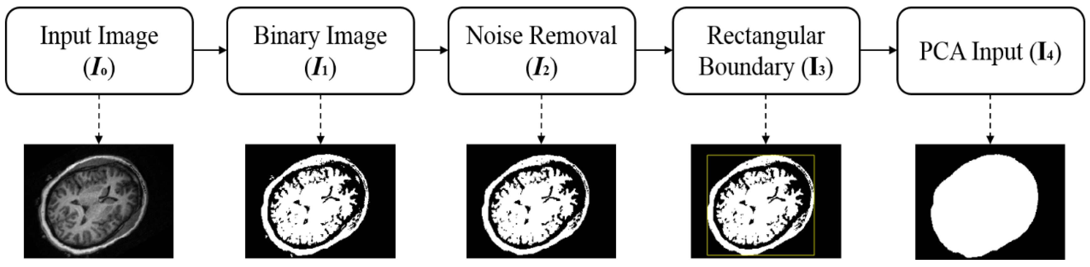
Due to the fact that the human brain is nearly elliptical, PCA is used, as it aligns the data in the direction of maximum variance (data spread). A reference 2-D slice Io is selected from the 3-D volume of the brain MRIs. The selection of the slice is important. As in fact, the higher slice (before and after the half of the total slices present in the volume), the brain in the 2-D image becomes more elliptical in shape. It can give a good estimate of the angle of brain symmetric axis as compared to other slices [43]. Therefore, a 1/55th slice of the total slices present in the volume of brain MRIs is considered as a reference slice. Next, the image is binarized [44] and noise is removed by a mathematical morphological filtering operation called area opening [45] (pp. 112–114). In this filtering procedure, small connected pixels of which the area (in a number of pixels) is less than a specified threshold (η) are removed. The value of “η” can be varied depending upon the type of brain MRIs and the extent of noise. After several experiments, a value of 100 pixels has been considered a good estimate for η (area threshold) in all the brain MRIs including tumor datasets. Mathematical, area opening is represented as:
where γη is the area opening, η is the value of threshold area of the connected pixels, and card(B) is the number of elements (cardinal number) of B.
Area opening is equivalently defined as the union of all the morphological opening (erosion followed by dilation) with the connected structuring element of which the size is equal to η. Then, a rectangular area is achieved by searching for the first and last nonzero pixels along the rows (top and bottom) and columns (left and right) of the noise-free binary image, as shown in Figure 2.
Some of the ROI pixels inside the rectangular boundary (image I3) have value 0. To make all the ROI pixels in the image I3 to one, the complement of noise-free binary image I2 is multiplied (logical AND) with the rectangular boundary, such that all the pixels inside the boundary are equal to 1 (Figure 3a). Largest connected component (LCC) is chosen (Figure 3b) from the resulted image and added (logical OR) to I3 (Figure 3c). Lastly, morphological flood-fill operation [45] (p. 208) is used to fill the holes (0-valued pixels) and achieved the binary image I4 with a single ROI. This image is exploited as an input for PCA (Figure 3d).
2.2.2. Principal Component Analysis
After noise removal and ROI extraction steps, the method uses 2-D coordinates (column and row) of the non-zero pixels of the object’s region as data points and an array X is formed as:
where r, c, and n represent row, column, and the total number of data points (1-valued pixels) in the ROI, respectively.
The size of X is n × 2, and rows of X are the location coordinate values of each non-zero pixel. Mean of X is a row vector mx (mean of the elements in each column of X), and can be computed as:
Similarly, a covariance matrix Px can be calculated as:
The mean subtraction is vital for performing PCA to ensure that the first principal component represents the direction of maximum variance. The covariance matrix Px is a real and symmetric matrix with a size of 2 × 2. Thus, finding a pair of orthonormal eigenvectors is always possible [46].
Suppose the elements of covariance matrix as:
where , , and .
The principal components can be determined by solving an eigenvalue problem as:
where , I, and e are the eigenvalue, identity matrix, and eigenvector, respectively.
If Equation (13) is to have a solution other than vector zero, then must be a nonsingular matrix. Therefore, it leads to a characteristics equation as:
After expansion of Equation (14), it becomes a second-degree equation as:
The Equation (15) can be solved using a quadratic formula as:
where and .
The corresponding eigenvectors of the eigenvalues can be calculated as:
where , and denote the eigenvectors and eigenvalues of , respectively.
The eigenvalues represent the length of the semi-axes of the ellipse and the eigenvectors specify the directions of these axes, as illustrated in Figure 4.
The rotation angle can be computed using the eigenvector corresponding to the largest eigenvalue as:
where are the horizontal and vertical components of the eigenvector associated with the largest eigenvalue, respectively.
This procedure provides a rough estimate of brain bilateral symmetric axis orientation θ1. Next, the slice is realigned with the vertical axis of the image using the angle θ1. Generally, it was observed that PCA aligned the brain bilateral symmetric axis with the vertical axis of the image with an error of less than 1°, as displayed in Figure 5.
The first row of Figure 5 indicates that bilateral symmetry axis of the brain is successfully aligned with the vertical axis (white vertical line) of the image by PCA, but sometimes as the second row in Figure 5 depicts, the bilateral symmetric axis of the brain is not completely aligned with the vertical axis of the image. Therefore, to ensure the accurate alignment of the bilateral symmetric axis of the brain with the vertical axis of the image, another fine alignment step is applied using a cross-correlation technique to find the angle θ2 with the vertical axis of the aligned image F (output of the previous step).
2.2.3. Cross-Correlation
In the cross-correlation technique, the aligned image F acquired in the last step is reflected about the current vertical center line to produce a new reflected image F′. The reflected image F′ is rotated by 2θ2 (θ2 ∈ [−10°, 10°]) with a 0.5° interval about the center of the image, cross-correlated with the image F, and the maximum correlation score is noted. The value of θ2 at which the cross-correlation score is maximum will be the required angle of bilateral symmetry with the vertical axis of the image. The cross-correlation is accomplished in the frequency space for greater efficiency. The detail of this method can be found in [18].
If θ2 is zero, it means that the PCA accurately aligns the brain bilateral symmetric axis with the vertical axis of the image, otherwise θr (yaw angle) will be:
where θ1 is the angle obtained from PCA and θ2 is the angle yielded from the cross-correlation technique.
After applying the cross-correlation technique, the brain bilateral symmetric axis is completely aligned with the vertical axis of the image, as displayed in Figure 5 (last column). Now, the angle θr can be used to estimate the first two parameters of the normal of required MSP plane using Equation (7), i.e., a = cos θ, and b = sin θ.
2.3. Fitting of Plane in Three Dimensions
According to Equation (4), the angle θr will be same for all the 2-D axial symmetric lines on each axial slice, irrespective of the position of slice Zr. Therefore, each image in the 3-D volume of the brain MRIs is rotated by an angle of −θr, so that bilateral symmetry axis of the brain becomes vertically oriented in each image. Normally, the translation offset pr of each symmetric axis can be computed using a cross-correlation of the aligned image with its vertical reflection about the center of the image [18,25]. This technique has two complications. The first one is the existence of outlier in the translation offset due to pathology effects, image artifacts, and symmetry axis ambiguity in the superior slices of brain. The second one is that this technique is also computationally intensive as it takes approximately 10 s for each slice of size (rows, column) 512 × 512 [18].
We have introduced a fast approach to estimating the translation offset independent of these constraints. The technique is based on the straightforward and effective observation that the head in the slices of brain MRIs is shaped like an ellipse (ellipsoid in three dimensions). Moreover, a trapezoid area on the surface of the head, center upon +x and −x (from ear to ear) directions of a height (30–45°) and a width (45–70°), has the most significant geometrical features as described by [16]. Fitting of plane consists of the following three steps:
1. Elliptical Area Extraction
The main objective to extract the elliptical area is to make the offset estimation independent of pathological effects, image artifacts, symmetry axis ambiguity in the higher slices, and computationally efficient. The aligned image is binarized [44] and noise is removed by the same procedure as described in the previous Section 2.2.1. Then, a rectangular area is achieved by searching for the first and last nonzero pixels along the rows (top and bottom) and columns (left and right) of the noise-free binary image (Figure 6d). First and last nonzero columns and rows are denoted by c1, c2, r1, and r2, respectively. Accordingly, the vertices of the rectangle are labeled as: A(c1, r1), B(c2, r1), C(c2, r2), and D(c1, r2), respectively.
Now, the parameters of an ellipse can be determined as:
Now, ellipse in parametric form can be written as:
Now, within I(i, j), which consists of all the pixels inside the elliptical boundary, the pixels are set to “1” based on Equation (25), as shown in Figure 6e,f, respectively.
2. Set of Mid-Parallel Lines Extraction
In the axial orientation, inferior and superior slices of the brain volume have ambiguous symmetry axes as compared to the slices near the center of the brain. Secondly, slices higher in the brain are almost ovals [16]. Therefore, ambiguous symmetry slices are automatically eliminated based on the ratio of the semi-axes of the ellipse, and only those slices of which this ratio is greater than 1.2 are extracted. This significantly improves the accuracy and efficiency of the algorithm. Selected sample slices with their respective elliptical area are illustrated in Figure 7.
The midline (principal axis) on each elliptical area slice is extracted using PCA as described in the preceding Section 2.2.2. An array Ar,s is formed from the location coordinates of three points (top, center, and bottom) on each midline (Figure 6f) as:
where r denotes the rth brain slice, s is the number of points considered on each midline, 1s is a column vector (s-dimensional) with all its elements equal to one, and N is equal to the total number of slices used (automatically selected).
The first column of Ar,s consists of pr (offset) values of the symmetric axis and the last column contains the indices of the respective slice. According to Equation (5), this makes an overdetermined set of linear equations in pr and Zr as a function of plane parameters c and d, as displayed in Figure 8. It can be solved by fitting a plane in 3-D Euclidean space to a set of parallel lines (midlines) having the orientation θr.
3. Fitting of Plane Using Orthogonal Regression
Orthogonal regression is employed using PCA to fit a plane to these midlines. PCA minimizes the orthogonal distances from the data point to the fitting plane (fitting model). In the linear case, it is also known as total least squares [42]. It is appropriate when all the variables are measured with errors. In contrary to the usual regression, where the assumption is that the predictor variables are measured precisely, and only the response variables have the component of error. Singular value decomposition (svd) is used to find the principal components of the PCA. The first step is to center the location data matrix Ar,s. This can be achieved by subtracting each data point of the matrix from its column mean. The resultant matrix is labeled as B. Then, the svd of B can be expressed as:
where U is a left-singular vector, S is a diagonal matrix of singular values, and V is a right-singular matrix.
The columns of V will be the required principal components. First two columns (first two principal components) of V define vectors that form a basis for the plane, and the third column (third principal component) is orthogonal to the first two principal components. The coefficients of the third principal component define the normal vector (n) of the MSP having an orientation of θr (yaw angle). The third coefficient of the normal vector n can be exploited to estimate the roll angle using Equation (7) as:
where c is the third coefficient of the normal vector.
Similarly, the parameter d of the MSP can be calculated by taking the scalar product of the normal vector n and the mean of Ar,s.
2.4. Transformation for Tilt Correction
After MSP normal vector computation, the translation matrix and the rotation matrix can be easily determined to correct the tilt (recenter and reorientation) of 3D-volume of brain MRIs. Let Rreq = yaw(θ)roll()pitch(ω) be the required rotation matrix, which can be written as:
where
The pitch (ω) angle will be zero for MSP, and yaw (θ) and roll () angles are calculated using Equations (19) and (28), respectively. The translation vector between the two coordinate systems, i.e., the center of the volume and centroid of the image grid, can be written as:
Trilinear interpolation is used to reslice the head volume after realignment and tilt correction.
3. Results and Discussion
The presented algorithm has been implemented in MATLAB 2018a on a PC with Intel(R) Core (TM) i5-6600 CPU @ 3.30 GHz, 8 GB RAM. Total time for all algorithmic steps is 1.04 s on average. No attempt has been made on optimization of the code. The developed algorithm has been tested on 157 real T1-weighted brain MRI datasets including 14 cases from the patients with the brain tumors. All the brain MRI datasets are publicly available. The details of the sample dataset images and parameters are given in Table 1. The first dataset is from Neurofeedback Skull-stripped (NFBS) repository [48] containing 125 volumes of brain MRI having several clinical and subclinical psychiatric syndromes. There is no ground truth (GT) for MSP available for this database. The second database is from the Internet Brain Segmentation Repository (IBSR) [49], containing 18 volumes of T1-weighted brain MRI with manually segmented hemispheres of the brain. The third dataset is from Montreal Neurological Institute’s Brain Images of Tumors for Evaluation (MNI BITE) database [50], which consists of 14 patients, 5 women and 9 men with a mean age of 52 years. The dataset includes 4 patients with low-grade gliomas (brain tumors) and 10 patients with high-grade gliomas (brain tumors). The mean tumor volume calculated manually by the experts was 30 cm3.
3.1. Evaluation on Real Datasets
The MSP is extracted from each dataset using the proposed algorithm and some slices perpendicular to the estimated MSP are snipped and displayed in Figure 9. The green line in each image is the intersecting line between the estimated MSP and the corresponding orthogonal slice. The first row (Figure 9a) represents the images from the NFBS database with extracted MSP by the proposed algorithm. The images of the same dataset (NFBS) are synthetically degraded by adding zero-mean Gaussian noise of several levels. Proposed algorithm breaking points can be found by incrementally adding the noise until the algorithm fails to detect the accurate MSP plane. The proposed algorithm successfully estimated the MSP at levels of noise up to SNR = −10.09 decibel (dB). The second row (Figure 9b) indicates representative resulting slices and the estimated MSP from noisy images. Images from the IBSR database are portrayed in Figure 9c. Manual delineation (GT) of brain hemispheres is available only for the IBSR database. The manual delineation boundary is superimposed on the input image with the white pixels by using a morphological gradient and binary skeletonization [51], as shown in Figure 9c. The proposed algorithm successfully extracts the MSP in all the volumes of the IBSR database and no obvious error is detected. The last two rows in Figure 9 contain the MSP-extracted results from the MNI BITE database. Group 2 (Figure 9d) comprises pre-operative MRIs and Group 3 (Figure 9e) includes MRIs acquired at different intervals of time, i.e., before and after surgery. Obvious asymmetries can be seen in the two groups of brain MRIs. The proposed algorithm extracted the symmetry axes from these volumes robustly and accurately.
3.2. Evaluation and Comparison on Synthetic Datasets
The accuracy of the proposed algorithm for extracting MSP is also evaluated by creating a set of 50 symmetrical scans of the real brain MRI from the NFBS database [48]. Each head scan is manually adjusted and perfectly aligned followed by reflecting one half of the head volume about the known MSP to form the other half. The two mirror halves are stitched together to create a symmetrical head scan with known GT MSP. The reason for creating such volumes is that perfectly symmetric head volumes with GT can be manipulated and transformed arbitrarily. In this way, we can avoid typical subjective factors of human visual inspection. Moreover, in reality, no human head scan exhibits perfect digital symmetry [52]. Therefore, GT in real brain MRIs cannot be used directly for MSP algorithm evaluation [18].
The presented algorithm results have been compared with a state-of-the-art MSP extraction method proposed by Ruppert et al. [27]. The algorithm is based on maximization of bilateral symmetry using 3-D Sobel edge operator, thresholding, downsampling, and a multiscale scheme. To improve the quantitative analysis of MSP identification, the authors also introduced a new MSP estimation error metric called average z-distance. The detail of this metric is discussed in the succeeding paragraph.
Metrics: Two metrics are measured to assess how accurately the algorithms detected the MSP. One is the angle difference (in degree) and is defined as the angle between normal vectors of GT MSP and estimated MSP. Mathematically, it can be computed using the inner product as:
where α is the angular difference, u is the normal vector of GT MSP, and v is the normal vector of calculated MSP.
When the two planes are parallel, this error metric is not sufficient and may be misleading due to translation between the estimated MSP and GT MSP. This problem is circumvented by Ruppert et al. [27] who proposed a new, simple, and fast metric known as average z-distance or z-score (in voxels), to measure MSP estimation error as a function of the distance between the two planes. This distance can be measured [27,33] by computing z coordinate from the plane equations, for the GT plane and the estimated plane, using each “x” and “y”. It can be written as:
where dim is the image dimension along x and y axes, and GT, and Est. stands for ground truth and estimated MSPs, respectively.
Both the algorithms (the proposed algorithm and Ruppert et al. algorithm) are evaluated for all the slices in the perfectly symmetrical head volume by determining their average z-distance with respect to each corresponding GT MSP. The mean z-scores obtained for both algorithms on 50 perfectly symmetric datasets are shown in Table 2.
The plot of average z-distance for the individual scan is illustrated in Figure 10. Ruppert et al. approach was unable to truly estimate the MSP in some scans and showed substantially large values for average z-distances, as indicated by the black square in Figure 10. These scans were not considered when measuring the mean z-score and the mean of angle differences, since they would synthetically intensify the z-score and standard deviation results of Ruppert et al. algorithm.
The values of z-score are almost similar as they reported in their paper, except for some scans having a rotation angle (either yaw or roll) of greater than 5°, as displayed in Figure 11. The situations at which their algorithm relied, i.e., smoothing, Sobel operator followed by thresholding of 5% brightest voxels, and symmetric score, are not satisfied in the presence of noise, image artifacts, and intensity inhomogeneity. This causes the offsets of plane underestimated. From Table 2, it is evident that Ruppert et al. algorithm accurately estimated the orientation of the MSP but failed to correctly calculate the offset of MSP. On the other hand, the proposed algorithm results are more consistent and accurate in orientations as well as in offsets.
To precisely inspect the accuracy of the proposed algorithm, many illustrative slices orthogonal to the estimated MSP are displayed in Figure 11. The lines in different colors (magenta, blue and green) are the intersecting lines between the extracted MSP and the respective orthogonal slice. The first column represents the input images and the second column shows the input images with the GT MSP intersection line (magenta color line). Similarly, third and fourth columns contain the images of Ruppert et al. and proposed algorithm results, respectively. Visual comparison in Figure 11 also reveals that the proposed algorithm outperformed Ruppert et al. algorithm in terms of accuracy, both in orientation and offsets. Ruppert et al. algorithm could not always achieve a rigorous estimate of MSP, particularly when the brain MRIs underwent a considerable transformation (rotation, translation, noise).
3.3. Evaluation and Comparison on Real Datasets
The proposed method has also been compared with Ruppert et al. method on real brain MRIs. Both techniques have been tested on 125 real head scans of the NFBS database [48] and 18 real head volumes of the IBSR database [49]. No GT for MSP is available for NFBS. Therefore, only visually comparison of the MSP extraction results has been reported for both the algorithms. The first row of Figure 12 shows some of the input image slices orthogonal to MSP.
Extracted MSP (green lines) using the proposed algorithm is displayed in the second row of Figure 12. Blue lines in the third row of Figure 12 displays the MSP extraction results of Ruppert et al. algorithm. The same pattern of the results in detecting MSP is shown by Ruppert et al. algorithm in real brain volumes. It estimates the orientation of the MSP more accurately but fails to correctly calculate the offset of MSP. On the other hand, the proposed algorithm detects the MSP more precisely and consistently.
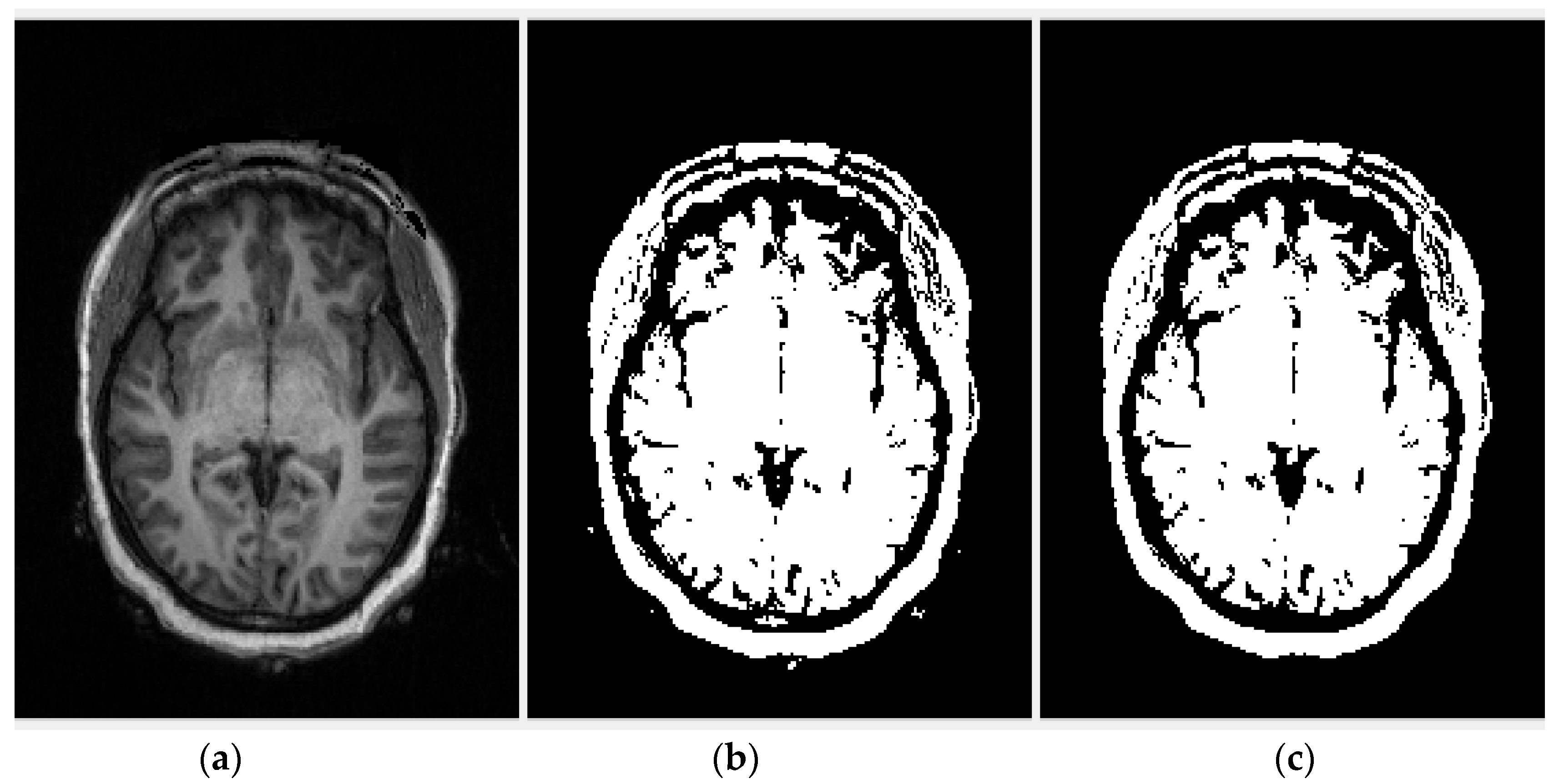
The IBSR database contains the manual delineation (GT) of brain hemispheres. For illustration, the input image from a brain volume is shown in Figure 13a with its manual delineation (mask) of the left (dark) and the right (bright) brain regions (Figure 13b). For comparison purpose, the boundary of the right region is superimposed on the input image with the white pixels using a morphological gradient and the binary skeletonization [51], as shown in Figure 13c. Therefore, this image is used as a GT for evaluation of MSP extraction results. For the precise and accurate result, the intersection line (between the estimated MSP and the corresponding orthogonal slice) should be overlapped or coincided with the white pixels boundary in the GT image.
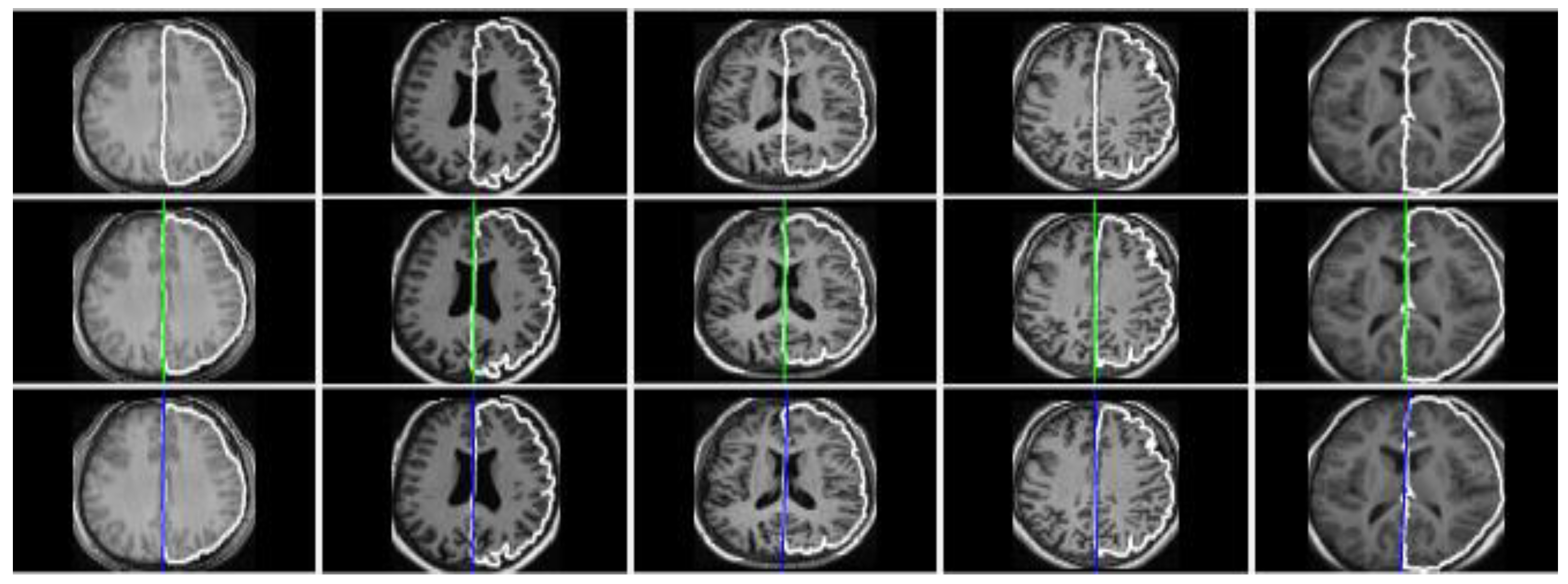
The first row in Figure 14 consists of all the input images with GT delineation of the right brain. Since the MSP divides the brain into two roughly symmetrical regions, the detected MSP (green line) by the proposed algorithm is almost completely overlapped with the boundary of the GT delineation of the right brain, as shown in the second row of Figure 14. In contrary, the MSP (blue line) estimated by Ruppert et al. algorithm is deteriorated significantly from the real boundary of the GT delineation of the right brain. Note that we did not compare results of brain tumors datasets with Ruppert et al. algorithm because they did not report results on such datasets in their paper.
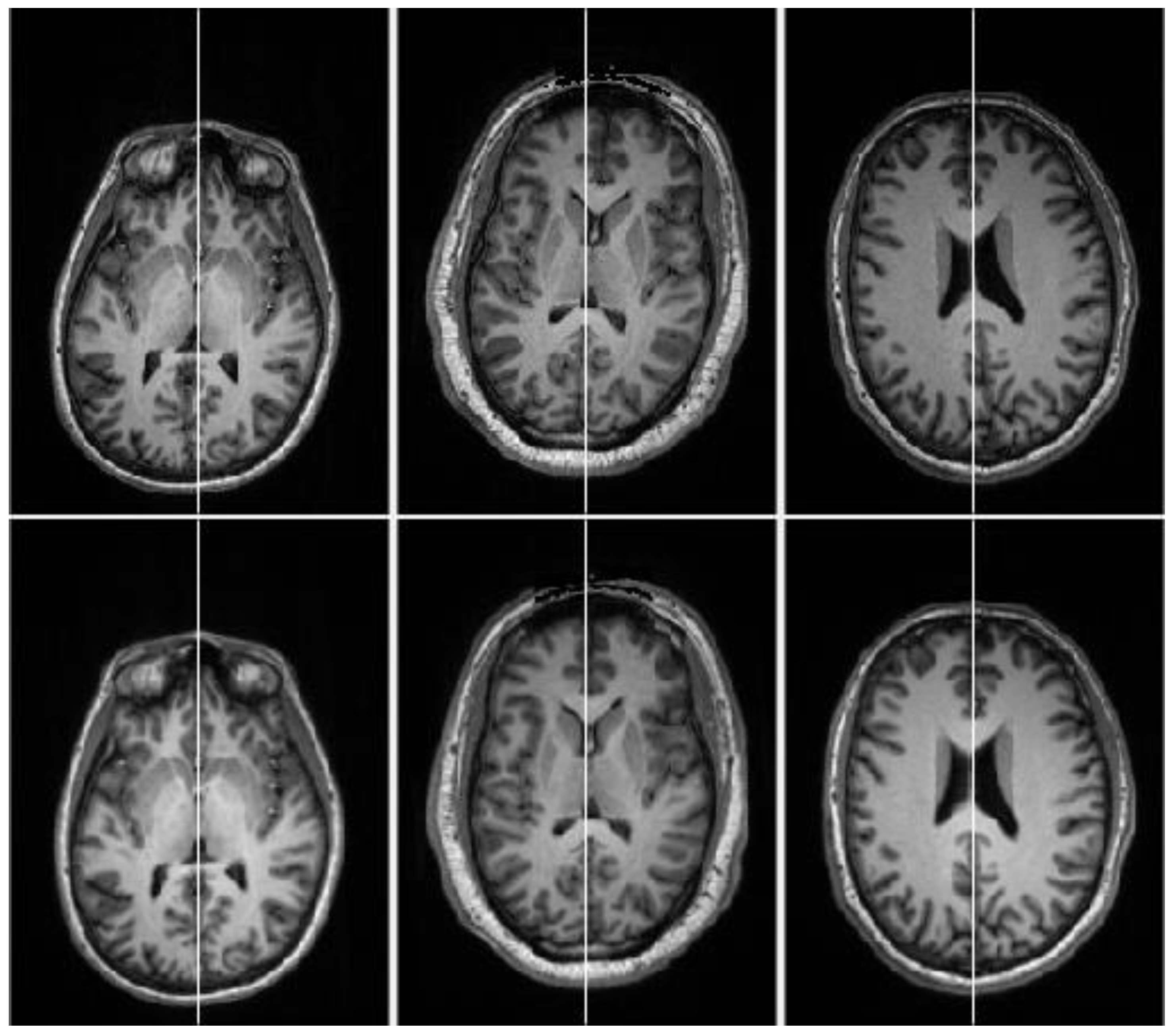
In short, all the promising results given by the proposed algorithm indicates that the developed technique has the highest accuracy and consistency in extracting the MSP. Finally, the results of automatic MSP detection and tilt correction (recenter and reorientation) in brain MRIs are displayed in Figure 15, where the first row represents the tilted slices of the three distinct brain volumes. After computing the parameters of the MSP and affine transformation, we reoriented and recentered the brain volumes. The corrected volume images are displayed in the second row of Figure 15.
4. Conclusions
In this paper, we have presented a fully automatic and computationally efficient MSP extraction and tilt correction technique in brain MRIs. The proposed method is based on PCA and symmetric features followed by plane fitting using orthogonal regression. Experimental results on 157 real heterogeneous brain MRIs including 14 datasets with brain tumors and comparison with a state-of-the-art method have confirmed that the proposed technique provides consistent performance with the highest accuracy. Moreover, it is 30 times faster than the competitor algorithm and takes only 1.04 s (on average) for all algorithmic steps per MRI volume. It is also robust on pathological brain MRIs having various intensity inhomogeneities, noises and image artifacts.
Some limitation of the proposed algorithm should be taken into consideration. The algorithm can only take T1-weighted MRI of the brain in axial orientation as an input. Although one can convert from one orientation (sagittal or coronal) to other using existing algorithms, the selection of brain slice in the first step can affect the yaw angle due to the assumption that it should be the same in each axial slice (see Equation (4)). The reason is that in the true anatomical structure of the brain, MSP is not exactly the plane but a curved surface even for a normal brain. Even though the planer estimation is adequate for many applications such as registration and symmetric/asymmetric analysis of brain images, the results obtained from the PCA in estimating the yaw angle can also affect the performance of the algorithm in the presence of high level of noise. When the SNR is less than −10.09 dB, estimates of the yaw angle cannot be trusted. This problem can be circumvented by increasing the angle range in the cross-correlation step. Our future work will include evaluation of the algorithm on brain images of various sources and modalities such as T2-weighted, Proton Density (PD) weighted, Fluid Attenuated Inversion Recovery (FLAIR), PET, and SPECT.
Author Contributions
H.Z.U.R. proposed the idea, implemented it and wrote the manuscript. S.L. supervised the study and manuscript-writing process.
Funding
This work was funded by the Korean Government (MSIP) under Grant No. 2015R1C1A1A01056013 and Grant No. 2012M3A6A3055694.
Acknowledgments
The author (H.Z.U.R.) is extremely thankful to the Higher Education Commission (HEC) of Pakistan for HRDI-UESTPs scholarship.
Conflicts of Interest
The authors declare no conflicts of interest.
References
- Davarpanah, S.H.; Liew, A.W.-C. Brain mid-sagittal surface extraction based on fractal analysis. Neural Comput. Appl. 2018, 30, 153–162. [Google Scholar] [CrossRef]
- Crow, T. Schizophrenia as an anomaly of cerebral asymmetry. In Imaging of the Brain in Psychiatry and Related Fields; Springer: Berlin, Germany, 1993; pp. 3–17. [Google Scholar]
- Oertel-Knochel, V.; Linden, D.E. Cerebral asymmetry in schizophrenia. Neuroscientist 2011, 17, 456–467. [Google Scholar] [CrossRef] [PubMed]
- Yu, C.-P.; Ruppert, G.C.; Nguyen, D.T.; Falcao, A.X.; Liu, Y. Statistical Asymmetry-based Brain Tumor Segmentation from 3D MR Images. Biosignals 2012, 15, 527–533. [Google Scholar]
- Roy, S.; Bandyopadhyay, S.K. Detection and Quantification of Brain Tumor from MRI of Brain and it’s Symmetric Analysis. Int. J. Inf. Commun. Technol. Res. 2012, 2, 477–483. [Google Scholar]
- Hermes, G.; Ajioka, J.W.; Kelly, K.A.; Mui, E.; Roberts, F.; Kasza, K.; Mayr, T.; Kirisits, M.J.; Wollmann, R.; Ferguson, D.J.P.; et al. Neurological and behavioral abnormalities, ventricular dilatation, altered cellular functions, inflammation, and neuronal injury in brains of mice due to common, persistent, parasitic infection. J. Neuroinflamm. 2008, 5, 48. [Google Scholar] [CrossRef] [PubMed] [Green Version]
- Schulte, T.; Muller-Oehring, E.M.; Rohlfing, T.; Pfefferbaum, A.; Sullivan, E.V. White Matter Fiber Degradation Attenuates Hemispheric Asymmetry When Integrating Visuomotor Information. J. Neurosci. 2010, 30, 12168–12178. [Google Scholar] [CrossRef] [PubMed] [Green Version]
- Kumar, A.; Schmidt, E.A.; Hiler, M.; Smielewski, P.; Pickard, J.D.; Czosnyka, M. Asymmetry of critical closing pressure following head injury. J. Neurol. Neurosurg. Psychiatry 2005, 76, 1570–1573. [Google Scholar] [CrossRef] [PubMed] [Green Version]
- Roussigné, M.; Blader, P.; Wilson, S.W. Breaking symmetry: The zebrafish as a model for understanding left-right asymmetry in the developing brain. Dev. Neurobiol. 2012, 72, 269–281. [Google Scholar] [CrossRef] [PubMed] [Green Version]
- Doi, K. Computer-aided diagnosis in medical imaging: Historical review, current status and future potential. Comput. Med. Imaging Graph. 2007, 31, 198–211. [Google Scholar] [CrossRef] [PubMed]
- Alves, R.S.; Tavares, J.M.R. Computer image registration techniques applied to nuclear medicine images. In Computational and Experimental Biomedical Sciences: Methods and Applications; Springer: Berlin, Germany, 2015; pp. 173–191. [Google Scholar]
- Lancaster, J.L.; Glass, T.G.; Lankipalli, B.R.; Downs, H.; Mayberg, H.; Fox, P.T. A modality-independent approach to spatial normalization of tomographic images of the human brain. Hum. Brain Mapp. 1995, 3, 209–223. [Google Scholar] [CrossRef]
- Minoshima, S.; Koeppe, R.A.; Frey, K.A.; Kuhl, D.E. Anatomic standardization: Linear scaling and nonlinear warping of functional brain images. J. Nucl. Med. 1994, 35, 1528–1537. [Google Scholar] [PubMed]
- Liu, S.X. Symmetry and asymmetry analysis and its implications to computer-aided diagnosis: A review of the literature. J. Biomed. Inform. 2009, 42, 1056–1064. [Google Scholar] [CrossRef] [PubMed]
- Prima, S.; Ourselin, S.; Ayache, N. Computation of the Mid-Sagittal Plane in 3D Medical Images of the Brain. In Proceedings of the 6th European Conference on Computer Vision-Part II, Dublin, Ireland, 26 June–1 July 2000; pp. 685–701. [Google Scholar]
- Liu, S.X.; Kender, J.; Imielinska, C.; Laine, A. Employing symmetry features for automatic misalignment correction in neuroimages. J. Neuroimaging 2011, 21, e15–e33. [Google Scholar] [CrossRef] [PubMed]
- Volkau, I.; Prakash, K.B.; Ananthasubramaniam, A.; Aziz, A.; Nowinski, W.L. Extraction of the midsagittal plane from morphological neuroimages using the Kullback–Leibler’s measure. Med. Image Anal. 2006, 10, 863–874. [Google Scholar] [CrossRef] [PubMed]
- Liu, Y.; Collins, R.T.; Rothfus, W.E. Robust midsagittal plane extraction from normal and pathological 3-D neuroradiology images. IEEE Trans. Med. Imaging 2001, 20, 175–192. [Google Scholar] [CrossRef] [PubMed] [Green Version]
- Kalavathi, P.; Senthamilselvi, M.; Prasath, V.B.S. Review of Computational Methods on Brain Symmetric and Asymmetric Analysis from Neuroimaging Techniques. Technologies 2017, 5, 16. [Google Scholar] [CrossRef]
- Brummer, M.E. Hough transform detection of the longitudinal fissure in tomographic head images. IEEE Trans. Med. Imaging 1991, 10, 74–81. [Google Scholar] [CrossRef] [PubMed]
- Guillemaud, R.; Marais, P.; Zisserman, A.; Mc Donald, T.; Crow, B. A 3-Dimensional midsagittal plane for brain asymmetry measurement. Schizophr. Res. 1995, 18, 183–184. [Google Scholar] [CrossRef]
- Nowinski, W.L.; Prakash, B.; Volkau, I.; Ananthasubramaniam, A.; Beauchamp, N.J., Jr. Rapid and automatic calculation of the midsagittal plane in magnetic resonance diffusion and perfusion images. Acad. Radiol. 2006, 13, 652–663. [Google Scholar] [CrossRef] [PubMed]
- Kuijf, H.J.; van Veluw, S.J.; Geerlings, M.I.; Viergever, M.A.; Biessels, G.J.; Vincken, K.L. Automatic extraction of the midsagittal surface from brain MR images using the Kullback–Leibler measure. Neuroinformatics 2014, 12, 395–403. [Google Scholar] [CrossRef] [PubMed]
- Ardekani, B.A.; Kershaw, J.; Braun, M.; Kanno, I. Automatic detection of the mid-sagittal plane in 3-D brain images. IEEE Trans. Med. Imaging 1997, 16, 947–952. [Google Scholar] [CrossRef] [PubMed]
- Prima, S.; Ourselin, S.; Ayache, N. Computation of the mid-sagittal plane in 3-D brain images. IEEE Trans. Med. Imaging 2002, 21, 122–138. [Google Scholar] [CrossRef] [PubMed]
- Bergo, F.P.; Ruppert, G.C.; Pinto, L.F.; Falcao, A.X. Fast and Robust Mid-Sagittal Plane Location in 3D MR Images of the Brain. In Proceedings of the BIOSIGNALS, Madeira, Portugal, 28–31 January 2008; pp. 92–99. [Google Scholar]
- Ruppert, G.C.; Teverovskiy, L.; Yu, C.-P.; Falcao, A.X.; Liu, Y. A new symmetry-based method for mid-sagittal plane extraction in neuroimages. In Proceedings of the 2011 IEEE International Symposium on Biomedical Imaging: From Nano to Macro, Chicago, IL, USA, 30 March–2 April 2011; pp. 285–288. [Google Scholar]
- Wu, H.; Wang, D.; Shi, L.; Wen, Z.; Ming, Z. Midsagittal plane extraction from brain images based on 3D SIFT. Phys. Med. Biol. 2014, 59, 1367–1387. [Google Scholar] [CrossRef] [PubMed]
- Zhang, Y.; Hu, Q. A PCA-based approach to the representation and recognition of MR brain midsagittal plane images. In Proceedings of the 30th Annual International Conference of the IEEEEngineering in Medicine and Biology Society, Vancouver, BC, Canada, 20–24 August 2008; pp. 3916–3919. [Google Scholar]
- Kalavathi, P.; Prasath, V.B.S. Automatic segmentation of cerebral hemispheres in MR human head scans. Int. J. Imaging Syst. Technol. 2016, 26, 15–23. [Google Scholar] [CrossRef]
- Ferrari, R.J.; Pinto, C.H.V.; Moreira, C.A.F. Detection of the midsagittal plane in MR images using a sheetness measure from eigenanalysis of local 3D phase congruency responses. In Proceedings of the 2016 IEEE International Conference on Image Processing (ICIP), Phoenix, AZ, USA, 25–28 September 2016; pp. 2335–2339. [Google Scholar]
- Descoteaux, M.; Audette, M.; Chinzei, K.; Siddiqi, K. Bone enhancement filtering: Application to sinus bone segmentation and simulation of pituitary surgery. Comput. Aided Surg. 2006, 11, 247–255. [Google Scholar] [CrossRef] [PubMed] [Green Version]
- de Lima Freire, P.G.; da Silva, B.C.G.; Pinto, C.H.V.; Moreira, C.A.F.; Ferrari, R.J. Midsaggital Plane Detection in Magnetic Resonance Images Using Phase Congruency, Hessian Matrix and Symmetry Information: A Comparative Study. In Proceedings of the International Conference on Computational Science and Its Applications, Melbourne, Australia, 2–5 July 2018; pp. 245–260. [Google Scholar]
- Toro, C.; Gonzalo-Martín, C.; García-Pedrero, A.; Menasalvas Ruiz, E. Supervoxels-Based Histon as a New Alzheimer’s Disease Imaging Biomarker. Sensors 2018, 18, 1752. [Google Scholar] [CrossRef] [PubMed]
- Caggiano, A. Tool Wear Prediction in Ti-6Al-4V Machining through Multiple Sensor Monitoring and PCA Features Pattern Recognition. Sensors 2018, 18, 823. [Google Scholar] [CrossRef] [PubMed]
- Cristalli, C.; Grabowski, D. Multivariate Analysis of Transient State Infrared Images in Production Line Quality Control Systems. Appl. Sci. 2018, 8, 250. [Google Scholar] [CrossRef]
- Zhang, J.; Feng, X.; Liu, X.; He, Y. Identification of Hybrid Okra Seeds Based on Near-Infrared Hyperspectral Imaging Technology. Appl. Sci. 2018, 8, 1793. [Google Scholar] [CrossRef]
- Wang, J.; Zhao, X.; Xie, X.; Kuang, J. A Multi-Frame PCA-Based Stereo Audio Coding Method. Appl. Sci. 2018, 8, 967. [Google Scholar] [CrossRef]
- Maalek, R.; Lichti, D.D.; Ruwanpura, J.Y. Robust Segmentation of Planar and Linear Features of Terrestrial Laser Scanner Point Clouds Acquired from Construction Sites. Sensors 2018, 18, 819. [Google Scholar] [CrossRef] [PubMed]
- Solomon, C.; Breckon, T. Fundamentals of Digital Image Processing: A Practical Approach with Examples in Matlab; John Wiley & Sons: Hoboken, NJ, USA, 2011; pp. 247–262. [Google Scholar]
- Mudrová, M.; Procházka, A. Principal component analysis in image processing. In Proceedings of the MATLAB Technical Computing Conference, Prague, Czech Republic, 4–8 July 2005. [Google Scholar]
- Petras, I.; Bednarova, D. Total Least Squares Approach to Modeling: A Matlab Toolbox. Acta Montan. Slovaca 2010, 15, 158–170. [Google Scholar]
- Minovic, P.; Ishikawa, S.; Kato, K. Symmetry Identification of a 3-D Object Represented by Octree. IEEE Trans. Pattern Anal. Mach. Intell. 1993, 15, 507–513. [Google Scholar] [CrossRef]
- Otsu, N. A threshold selection method from gray-level histograms. IEEE Trans. Syst. Man Cybern. 1979, 9, 62–66. [Google Scholar] [CrossRef]
- Soille, P. Morphological Image Analysis: Principles and Applications, 2nd ed.; Springer Science & Business Media: Berlin/Heidelberg, Germany, 2013. [Google Scholar]
- Noble, B.; Daniel, J.W. Applied Linear Algebra; Prentice-Hall: Upper Saddle River, NJ, USA, 1988; Volume 3. [Google Scholar]
- Liu, Y.; Collins, R.T.; Rothfus, W.E. Automatic Extraction of the Central Symmetry (Mid-Sagittal) Plane from Neuroradiology Images; Carnegie Mellon University, The Robotics Institute: Pittsburgh, PA, USA, 1996. [Google Scholar]
- Puccio, B.; Pooley, J.P.; Pellman, J.S.; Taverna, E.C.; Craddock, R.C. The preprocessed connectomes project repository of manually corrected skull-stripped T1-weighted anatomical MRI data. Gigascience 2016, 5, 45. [Google Scholar] [CrossRef] [PubMed]
- Internet Brain Segmentation Repository (IBSR). Massachusetts General Hospital. Available online: http://www.nitrc.org/projects/ibsr/ (accessed on 26 September 2018).
- Mercier, L.; Del Maestro, R.F.; Petrecca, K.; Araujo, D.; Haegelen, C.; Collins, D.L. Online database of clinical MR and ultrasound images of brain tumors. Med. Phys. 2012, 39, 3253–3261. [Google Scholar] [CrossRef] [PubMed]
- Gonzalez, R.C.; Woods, R.E. Digital Image Processing (Global Edition), 4th ed.; Pearson: New York, NY, USA, 2018; pp. 747–750. [Google Scholar]
- Zhao, L.; Ruotsalainen, U.; Hirvonen, J.; Hietala, J.; Tohka, J. Automatic cerebral and cerebellar hemisphere segmentation in 3D MRI: Adaptive disconnection algorithm. Med. Image Anal. 2010, 14, 360–372. [Google Scholar] [CrossRef] [PubMed]
Figure 1.
An ideal coordinate system XoYoZo (black) versus an imaging coordinate system XYZ (blue).

Figure 2.
Steps for noise removal and region of interest (ROI) extraction.

Figure 3.
Intermediate steps between images I3 and I4, (a) logical AND of I2 with the rectangular boundary, (b) largest connected component, (c) logical OR of (b) with I3, (d) holes filling using morphological flood-fill operation.
Figure 3.
Intermediate steps between images I3 and I4, (a) logical AND of I2 with the rectangular boundary, (b) largest connected component, (c) logical OR of (b) with I3, (d) holes filling using morphological flood-fill operation.

Figure 4.
Orthonormal eigenvector by principal component analysis (PCA). (a) Eigenvector e1 through the center of the elliptical area represents the maximum variance and e2 is perpendicular to e1, and (b) extracted eigenvectors from brain brain magnetic resonance images (MRI) are imposed on the image.

Figure 5.
Estimation of symmetry axis orientation θr. First column: input images; second column: alignment of the brain bilateral symmetry axis with the vertical axis of the image using θ1; last column: brain bilateral symmetry axis alignment using θr = θ1 + θ2. Note that θ2 = 0 in the first row.
Figure 5.
Estimation of symmetry axis orientation θr. First column: input images; second column: alignment of the brain bilateral symmetry axis with the vertical axis of the image using θ1; last column: brain bilateral symmetry axis alignment using θr = θ1 + θ2. Note that θ2 = 0 in the first row.

Figure 6.
Elliptical area extraction. (a) Input image, (b) binary image, (c) noise removal, (d) rectangular boundary extraction, (e) elliptical area extraction, and (f) symmetric axis (midline) extraction using PCA.
Figure 6.
Elliptical area extraction. (a) Input image, (b) binary image, (c) noise removal, (d) rectangular boundary extraction, (e) elliptical area extraction, and (f) symmetric axis (midline) extraction using PCA.


Figure 7.
Selected slices from a 3-D volume of brain MRIs. (a) Selected slices based on semi-axes, and (b) extracted elliptical area from slices.
Figure 7.
Selected slices from a 3-D volume of brain MRIs. (a) Selected slices based on semi-axes, and (b) extracted elliptical area from slices.

Figure 8.
The relationship between the brain slice position (Zr) and the symmetric axis offset (pr). The illustration is adapted from [47].
Figure 8.
The relationship between the brain slice position (Zr) and the symmetric axis offset (pr). The illustration is adapted from [47].

Figure 9.
Visual comparison of the proposed algorithm in extracting the symmetric axis (MSP) from real brain MRIs, (a) the NFBS database [38], (b) images of the same subjects with Gaussian noise, (c) the IBSR database [39], (d) the MNI BITE database Group 2, and (e) the MNI BITE database Group 3 [40].

Figure 10.
Average z-distances of perfectly symmetric datasets (z-distances indicated by the square are not included for mean z-score calculation).
Figure 10.
Average z-distances of perfectly symmetric datasets (z-distances indicated by the square are not included for mean z-score calculation).

Figure 11.
Visual comparison of the proposed algorithm with Ruppert et al. algorithm for extracting the symmetric axis (MSP) from perfectly symmetric datasets: (a) input slice, (b) ground-truth slice, (c) Ruppert et al. [27] algorithm results, and (d) proposed algorithm results.
Figure 11.
Visual comparison of the proposed algorithm with Ruppert et al. algorithm for extracting the symmetric axis (MSP) from perfectly symmetric datasets: (a) input slice, (b) ground-truth slice, (c) Ruppert et al. [27] algorithm results, and (d) proposed algorithm results.

Figure 12.
Visual comparison of the proposed algorithm with Ruppert et al. algorithm for extracting the symmetric axis (MSP) from real head volumes (the NFBS database [48]). First row, second row, and third row display the input images, the proposed algorithm results, and Ruppert et al. algorithm results, respectively.

Figure 13.
Superimposition of the ground truth (GT) image on the input image of the IBSR dataset [49]: (a) input image; (b) GT image; and (c) boundary of the right brain region is imposed on the input image with the white pixels.
Figure 13.
Superimposition of the ground truth (GT) image on the input image of the IBSR dataset [49]: (a) input image; (b) GT image; and (c) boundary of the right brain region is imposed on the input image with the white pixels.

Figure 14.
Visual comparison of the proposed algorithm with Ruppert et al. algorithm for extracting the symmetric axis (MSP) from real head volumes of the IBSR database [49]. First row, second row, and third row display the input images, the proposed algorithm results, and Ruppert et al. algorithm results, respectively.

Figure 15.
The results of symmetric detection and tilt correction (realignment of the brain head volume). The input head volumes images are in the first row and reoriented (recentered) head volumes images are in the second row.
Figure 15.
The results of symmetric detection and tilt correction (realignment of the brain head volume). The input head volumes images are in the first row and reoriented (recentered) head volumes images are in the second row.


Table 1.
Datasets used for evaluation.
| Datasets | Detail of Images |
|---|---|
| NFBS [48] | There are 125 T1-weighted MRI scans, 77 females and 48 males in the 21–45 age range (average: 31) with a variety of clinical and subclinical psychiatric symptoms. The size of the individual scan is 256 × 256 × 192 and each voxel size is 1 × 1 × 1 mm3. The first two dimensions in each scan size indicate the individual image size (rows, columns) and the third dimension represents the number of images in the scan. |
| IBSR [49] | Eighteen volumes of T1-weighted brain MRI from all age groups from juvenile to adult are available online with ground truth. The size of the individual scan is 256 × 256 × 128 and each voxel size is 1.5 × 1.5 × 1.5 mm3. Most of the scans in this database have low-contrast images. |
| MNI BITE [50] | Real T1-weighted brain MRI of 14 patients with brain tumors (gliomas). We have used scans from Group 2 (pre-operative MRIs) and Group 3 (post-resection MRIs). The size of each scan in Group 2 is 394 × 466 × 378. Group 3 contains scans of different sizes and dimensions. |
Table 2.
Quantitative results comparison for perfectly symmetric datasets.
| Ruppert et al. Algorithm | Proposed Algorithm | |||||
|---|---|---|---|---|---|---|
| z Score (Voxels) | Angle Difference (°) | Time (s) | z-Score (Voxels) | Angle Difference (°) | Time (s) | |
| Mean | 1.246 | 0.10 | 35.02 | 0.336 | 0.06 | 1.04 |
| Std. | 2.041 | 0.22 | 1.12 | 0.324 | 0.21 | 0.02 |
| Median | 0.50 | 0.00 | 34.86 | 0.250 | 0.00 | 1.01 |
© 2018 by the authors. Licensee MDPI, Basel, Switzerland. This article is an open access article distributed under the terms and conditions of the Creative Commons Attribution (CC BY) license (http://creativecommons.org/licenses/by/4.0/).
Share and Cite
MDPI and ACS Style
Rehman, H.Z.U.; Lee, S. An Efficient Automatic Midsagittal Plane Extraction in Brain MRI. Appl. Sci. 2018, 8, 2203. https://doi.org/10.3390/app8112203
AMA Style
Rehman HZU, Lee S. An Efficient Automatic Midsagittal Plane Extraction in Brain MRI. Applied Sciences. 2018; 8(11):2203. https://doi.org/10.3390/app8112203
Chicago/Turabian StyleRehman, Hafiz Zia Ur, and Sungon Lee. 2018. "An Efficient Automatic Midsagittal Plane Extraction in Brain MRI" Applied Sciences 8, no. 11: 2203. https://doi.org/10.3390/app8112203
Note that from the first issue of 2016, this journal uses article numbers instead of page numbers. See further details here.