A Unified Approach to Design Robust Controllers for Nonlinear Uncertain Engineering Systems

Department of Electrical Engineering and Information Technology, University of Naples Federico II, Via Claudio 21, 80125 Napoli, Italy
Appl. Sci. 2018, 8(11), 2236; https://doi.org/10.3390/app8112236
Submission received: 25 September 2018
/
Revised: 24 October 2018
/
Accepted: 5 November 2018
/
Published: 13 November 2018
Abstract
:Featured Application
Design and realization of robust, simple and effective controllers, mainly for the transportation and manufacturing systems.
Abstract
This paper presents new theorems, which allow to design in a unified way robust proportional-derivative (PD)-type control laws without chattering for a broad class of uncertain nonlinear multi-input multi-output (MIMO) systems, subject to bounded disturbances and noises, of great theoretical and engineering relevance. These controllers are used to track a reference signal with bounded second derivative with the tracking error norm smaller than a prescribed value. The proposed control laws are simple to design and implement, above all for robotic systems, both in the case of a trajectory assigned in the joint space and in the workspace. The obtained theoretical results can have numerous applications. In this paper four significant applications are provided. The first one concerns the solution of a nonlinear equations system or the determination of an equilibrium point of a nonlinear system. The second case study deals with the inversion of a nonlinear vectorial function or the kinematic inversion of a robot. The third application concerns: (A) the tracking control of a robot with parametric uncertainties, with and without measurement noise on velocity, both in the joint space and the workspace; (B) the impedance control of a robot interacting with a human operator. The fourth case study addresses the tracking control of an uncertain nonlinear system that does not belong to the class of mechanical systems. Finally, an appendix is included, providing six easy examples, which show how the results proposed in the paper can eliminate and/or reduce serious disadvantages existing in the robust control literature for significant classes of linear and nonlinear uncertain systems.
1. Introduction
Since a kilowatt-hour of electrical energy transformed into mechanical energy can produce an impressive amount of human work, current and future well-being depend primarily on automatic systems concerning many key areas for humanity, including the transportation and manufacturing systems.
Hence, it is of great relevance to develop control algorithms that can be easily implemented using modern digital and wireless technologies to force electromechanical systems to behave like skilled workers who work quickly, accurately, and cheaply despite parametric variations, nonlinearities, and persistent disturbances. In particular, special attention has been paid to solving robust tracking control problems, which resulted in a considerable number of publications (see, e.g., [1,2,3,4,5,6,7,8,9,10,11,12,13,14,15,16,17,18,19,20,21,22,23,24,25,26,27,28,29,30,31,32,33,34,35,36,37,38,39,40,41,42,43] and references therein). However, there exist many results obtained under the following simplified hypotheses, which are not always realistic and feasible: (1) exact knowledge of the controlled system is assumed; (2) actuators are considered ideal; and (3) signals are assumed measurable without noises, therefore, ideal or almost ideal derivative actions can be used.
The robust tracking control mostly uses the well-known feedback linearization, inverse model and model predictive control (MPC) techniques.
Feedback linearization is the process of determining a feedback law and a change of coordinates that transform a nonlinear system into a linear and controllable one.
Inverse modeling is a general mathematical method to determine unknown causes on the basis of observation of their effects, as opposed to modeling of direct problems whose solution involves finding effects on the basis of a description of their causes.
MPC is a very popular controller design method in the process industry for discrete-time models.
Taking also into account that the computation time for feedback linearization or control signal generation by the inverse model or MPC techniques is non-negligible, these simplified hypotheses make the above mentioned techniques not always reliable (see [4,5,6,8,10,14,15,20,23,24,25,29,31,33,37,40,41]. In some cases, the control system can even be unstable, as can be verified with simple examples (see also Appendix A). Furthermore, the control techniques using high-frequency and high-amplitude control signals do not yield good performance (see also Appendix A).
To avoid the aforementioned problems, various modifications of the inverse model and feedback linearization techniques have been proposed, for instance, a computed-torque-like control with variable-structure compensation (see [20,25,26]), which is, however, difficult to design and implement and also presents high-frequency oscillations (see also Appendix A).
Thus, there is still a demand for smooth robust controllers that allow a plant belonging to a broad class of nonlinear uncertain systems, including electromechanical ones, to track a sufficiently smooth reference signal with a tracking error norm smaller than a prescribed value, despite the presence of disturbances and parametric and structural uncertainties, using real actuators and real derivative actions.
In some previous author’s contributions (see [21,34,35]) some control methodologies of MIMO uncertain linear systems and of a class of MIMO nonlinear uncertain systems have been provided in order to design simple controllers: state feedback controller with integral action, a pseudo-PD and pseudo-proportional-integral-derivative (pseudo-PID) to track sufficiently smooth trajectories with an a priori given maximum error.
Moreover, in [38], for three classes of uncertain nonlinear MIMO systems, that are wider with respect to [21,34,35], including several manufacturing systems and land, sea and air transportation systems, subject to nonstandard disturbances and noises, some theorems are proved, that allow to design pseudo-PID controllers to track a sufficiently smooth reference signal with the tracking error norm smaller than a prescribed value.
This paper, for a broad class of uncertain nonlinear MIMO systems much more general with respect to [34,35,38], provides a new and unified approach to design robust PD-type control laws without chattering to track a reference signal with bounded second derivative with the tracking error norm smaller than a prescribed value, despite the presence of bounded disturbances, parametric and structural uncertainties, and bounded measurement noises. With respect to [34], it is also proved that the proposed control laws are robust with respect to bounded measurement noises.
With reference to the mechanical and transportation systems, this theory can be successfully applied when the controller uses as information: signals related to the joint space (obtainable with encoders, resolvers, or tachometric dynamos, for example) or signals related to the workspace (e.g., obtainable with cameras, sonar, or global positioning system (GPS)). Moreover, the proposed results are very useful also for the control of human-machine interaction (see e.g., [8,15,28]).
The proposed control laws are based on the concept of majorant systems and result in establishing asymptotic bounds for the tracking error and its first derivative. The proposed controller design is based on two parameters. The first parameter is related to the minimum eigenvalue of a suitable matrix, on which the practical stability depends. The second parameter is easily related to the practical asymptotic stability region, the desired maximum tracking error norm, and its convergence velocity. If the tracked trajectories are not sufficiently smooth, suitable filtering laws are proposed to facilitate the implementation of the control laws and reduce the control magnitude, particularly during the transient phase.
The designed controllers using the developed majorant systems technique allow one to obtain, in general, less conservative results; i.e., the actual tracking error is quite close to the error computed with the proposed methodology, unlike many other approaches based on unsuitable Lyapunov functions. This enables one to avoid significant technological problems such as, e.g., oversized amplifiers and actuators.
The obtained theoretical results can be successfully applied to numerous theoretical and engineering applications (e.g., control of: rolling mills, conveyor belts, automatic guided vehicles (AGVs), unicycles, cars, trains, ships, airplanes, drones, missiles, satellites, manufacturing robots—welding, painting, assembly, pick and place for printed circuit boards, packaging and labeling, palletizing, product inspection, and testing-, surgical robots).
The above systems are of great engineering relevance, e.g., nowadays AGVs have revolutionized the logistics and production organization, as they are innovative, versatile and cheap mobile robots very used in various processes (production and management of warehouses) for the loading, unloading, and/or transportation purposes.
All the above mentioned systems fall into the considered broad class of systems and, therefore, can be effectively and simply controlled with the proposed laws in realistic situations and also by technicians not expert in the control field (see the easy and efficient control of the simple AGV considered in the Appendix A and, above all, the second and third applications in the paper).
Concerning this, in the paper four significant applications are provided.
The first one concerns the solution of a nonlinear equations system or the determination of an equilibrium point of a nonlinear systems. The second case study deals with the inversion of a nonlinear vectorial function or the kinematic inversion of a robot. The third application concerns: (A) the tracking control of a robot with parametric uncertainties, with and without measurement noise on velocity, both in the joint space and the workspace; and (B) the impedance control of a robot interacting with a human operator. The fourth case study addresses the tracking control of an uncertain nonlinear system that does not belong to the class of mechanical systems and to the classes of systems considered in [34,35,38].
Finally, it is included an appendix in which six easy examples are provided. The first five ones clearly show how numerous control techniques available in the literature (e.g., [10,14,15,20,23,24,25,29,31,33,41,42,43] and the references therein) for significant classes of linear and nonlinear systems can produce unstable control system or can significantly reduce the performance of the control system, under the following realistic hypotheses: parametric uncertainties, real actuators, measurement noise, finite online computation time of the control signal.
The sixth example shows that the above mentioned disadvantages can be eliminated and/or reduced with the results proposed in the paper.
This paper is organized as follows. The considered class of systems, the problem statement and theoretical background, including the majorant systems technique and some theorems useful to easily determine a majorant system of a nonlinear uncertain system with bounded uncertainties, are given in Section 2. Section 3 provides the main results, including the tracking control law and the corresponding tracking error bounds. Four case studies, of theoretical and engineering relevance, are presented in Section 4. Section 5 outlines the main contributions and future developments. Finally, an appendix provides simple five counter-examples and a sixth example, that shows the utility of the proposed results to eliminate and/or reduce serious disadvantages existing in the robust control literature in the presence of parametric uncertainties, real actuators, measurement noise, finite online computation time of the control signal, thus concluding this paper.
2. Problem Formulation and Preliminaries
Consider the uncertain nonlinear dynamic system, much more general with respect to [34,35,38]:
where is the time, is the output, , is the input, is a bounded disturbance, is the vector of the uncertain parameters, is a nonlinear bounded matrix function of rank and is a nonlinear vector function satisfying the following conditions.
(1) Positivity condition: there exists a matrix such that:
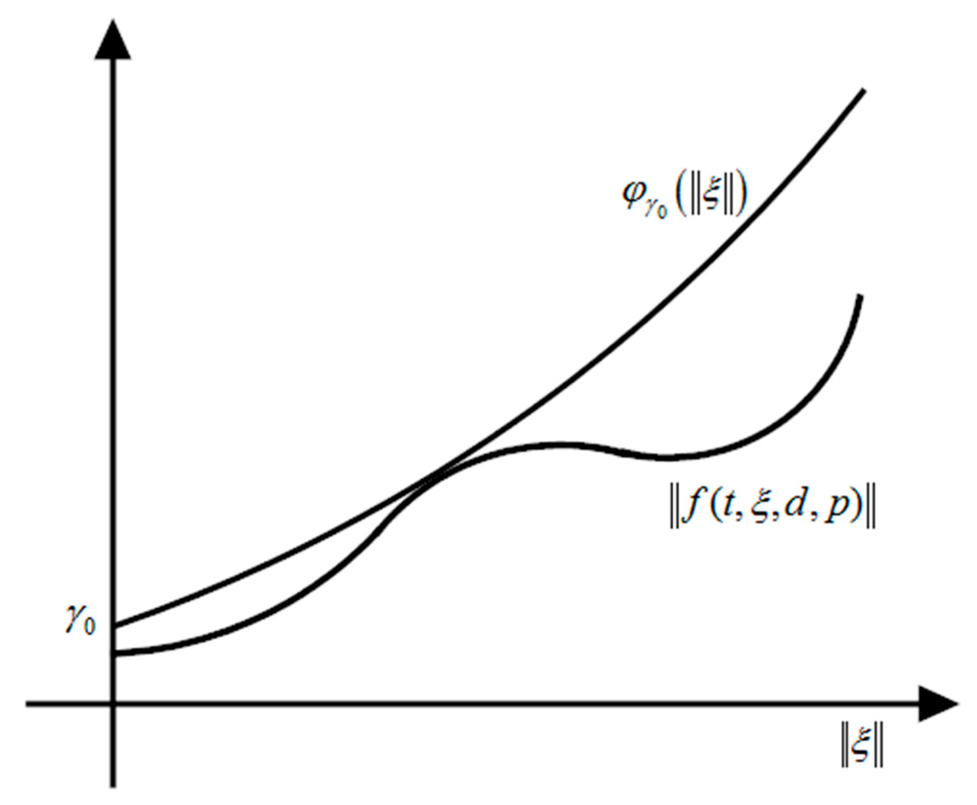
(2) Bounding condition of class there exists a continuous function , non decreasing and with initial value said of class such that (see Figure 1).
There exist several classes of systems whose models, after:
- (a)
- a possible appropriate changing of variable and/or;
- (b)
- the use of a possible appropriate compensation signal dependent on and/or;
- (c)
- possible appropriate mathematical steps by using the derivative of Lie, are of type (1). In the following five significant classes of the above systems are reported.
Class 1.
Note that many mechanical systems with m degrees of freedom (e.g., cars, trains, conveyor belts, manufacturing machineries, and the Cartesian robots) are described by the equation:
whereis the generalized coordinate vector,is the generalized control forces vector,is the generalized gravity forces vector,is the generalized disturbance forces vector,,with ,are, respectively, the inertia matrix, damping matrix, stiffness matrix and transmission matrices of the generalized forcesandand, finally,is the vector of the uncertain parameters. It can be readily verified that the mechanical system (4) is of type (1) and can satisfy the conditions (2) and (3).
Class 2.
Note that many mechanical systems with m degrees of freedom are described by the equation:
whereis the velocity vector,is the generalized control forces vector,is the generalized gravity and disturbance forces vector,are, respectively, the inertia matrix and damping matrix, andis the vector of the uncertain parameters.
By activating system (5) with a real actuator described by equation:
where is the actuator input (e.g., the actuator supply voltage), is the dynamic matrix, is the input matrix of full rank, is the interaction matrix, and is the vector of the uncertain parameters.
Combining the Equations (5) and (6) yields:
from which:
It is easy to verify that the electromechanical system (8) is of type (1) and that it can satisfy conditions (2) and (3).
Class 3.
Note that many robots, satellites, drones, and ships with m degrees of freedom can be represented by the equation:
whereis the generalized coordinate vector,is the generalized control forces vector,is the generalized gravity forces vector,is the generalized disturbance forces vector,is the inertia matrix,is the vector of the damping, centrifugal and Coriolis forces,is the vector of the possible stiffness forces,with,are transmission matrices of the generalized forcesand, and, finally,is the vector of the uncertain parameters.
It is easy to verify that system (9) is of type (1) and that it can satisfy conditions (2) and (3).
Class 4.
Consider the system:
whereis the state,is the input,is the output,is the disturbance,are matrices of appropriate dimensions,is a nonlinear vector function andis the vector of the uncertain parameters. If:
it is:
It can be readily verified that system (13) is of type (1) and it can satisfy conditions (2) and (3).
Class 5.
Consider the transformation:
e.g., the coordinate transformation between the joint space and the workspace of a robot or consider the nonlinear equationconstant.
Let a generic trajectory with bounded second derivative, it is:
Moreover:
By setting it can be verified that (16) is of type
Hence the model of the inversion error of the transformation is of type (1), satisfies condition (2), and it can satisfy condition (3).
A possible control law, to force plant (1) to track a reference signal with bounded second derivative, is:
where , , and is a possible compensation signal, e.g., where or , is the pseudo-inverse of and are the nominal values of .
Remark 1.
A reference signalwith bounded second derivative can be obtained by interpolating a set of given pointswith quadratic or cubic splines or by filtering any piecewise constant or piecewise linear signalwith the following MIMO filter:
In this way, sinceis available, the derivative action of the controller can be avoided, ifis measurable. Moreover, by suitably choosing the initial conditions of the filter and its cutoff frequency, it is possible to reduce the control action, above all during the transient phase.
By setting:
the plant (1) with the control law (18) is described by the following equations:
where:
To design the control law (18) in order to force plant (1) to track a reference signal with bounded second derivative, with tracking error norm smaller that a prescribed value, despite the presence of parametric and/or structural uncertainties and bounded disturbances, the following preliminary notations, definitions and lemmas are introduced.
where is a symmetric and positive definite (p.d.) matrix, is the transpose of , is a compact set, is the maximum (minimum) eigenvalue of a square matrix with real eigenvalues.
Definition 1.
Given the system:
a constantand asymmetric matrixA positive first-order system:
where, such that,,andis said to be a majorant system of the system (24).
Remark 2.
It is worth noting that a majorant system of a system belonging to the class of the uncertain time-variant nonlinear systems (24) (which of course includes also the class of linear uncertain systems) is a time-invariant first-order system. So it can be used to easily solve numerous analysis and synthesis problems, such as the analysis of practical stability, the robust stabilization, the robust tracking (see also [21,34,35,38]).
Lemma 1.
Letbe a symmetric p.d. matrix,be a symmetric matrix,, , , be a compact subset of,be a vector continuous with respect toandbe a matrix of rankandbe a matrix of rank m. Then,and, the following inequalities hold:
Proof.
See Lemmas 1 and 3 in [21]. ☐
Lemma 2.
Consider a matrix function, with, defined as a ratio of a multi-affine matrix function to a multi-affine non null polynomial:
whereand. Suppose thatis an hyper-rectangle given by.
Then, is attained in one of the vertices of .
Proof.
The proof follows from Theorem 1 in [44] by setting and . ☐
Lemma 3.
Let:
be a matrix function, ratio of a quadratic matrix function to a quadratic non null polynomial with respect to the parameters . Then a lower estimate of(an upper estimate of) is given by, whereis the set ofvertices of andis obtained from matrixby replacingwith the product,.
Proof.
The proof follows from Corollary 1 in [44] by setting and . ☐
Lemma 4.
Let:
be anonsingular function matrix, where,,is a compact set and each functionis continuous with respect toThen, a lower estimate of(an upper estimate of) is given by(), which is attained in one of the vertices of .
Proof.
The proof follows from Corollary 2 in [44] by setting and . ☐
Lemma 5.
Letbe a symmetric p.d. matrix,a reference signal with bounded second derivative anda compensation signal such that. Then ifwhereandis a function of classthen:
whereandis a function of class, with.
Proof.
Note that Hence:
☐
3. Main Results
This section presents the main theorems and results, providing a general approach to designing smooth robust controllers for a system (1) to track a sufficiently smooth reference signal with error norm smaller than a prescribed value.
Theorem 1.
Consider the uncertain nonlinear dynamic system (1), satisfying conditions (1), (2) and controlled with the control law (18), i.e., the following:
where:
Then, ifis bounded and the possible compensation signalis such thata majorant system of the closed loop system (34) is:
where, with:
andis a function of class, with.
Proof.
By choosing as “Lyapunov function” the quadratic form , for belonging to the generic hyper-circumference , its derivative satisfies the following inequalities:
from which, for (26) and (27) of Lemma 1, it follows that:
Since:
if , after certain mathematical steps, then:
Moreover, it is easy to verify that:
hence:
The proof follows from (43), from (32) of Lemma 5 and by noting that, for x belonging to the generic hyper-circumference from (28) of Lemma 1 and (42) it is:
☐
Theorem 1 allows one to establish the following significant theorems.
Theorem 2.
Consider the system (34). If hypotheses of Theorem 1 are satisfied then, for, the following inequalities hold:
whereis the value offor which the lineis tangent to the curveand,are the smallest equilibrium points of the majorant system (36) (see Figure 2).
Proof.
The proof easily follows by using the Lyapunov function or by noting that in the interval is decreasing (see Figure 2, as well). ☐
It is worth noting that for sufficiently large from Theorem 2 it is Hence, for sufficiently large , if then:
Remark 3.
From (46) and Theorem 2 it follows that, for sufficiently largeand for sufficiently large, the error norm decreases with respect to parameterwith an almost quadratic behavior, and the derivative error norm decreases, always with respect to parameter, with an almost linear behavior.
Remark 4.
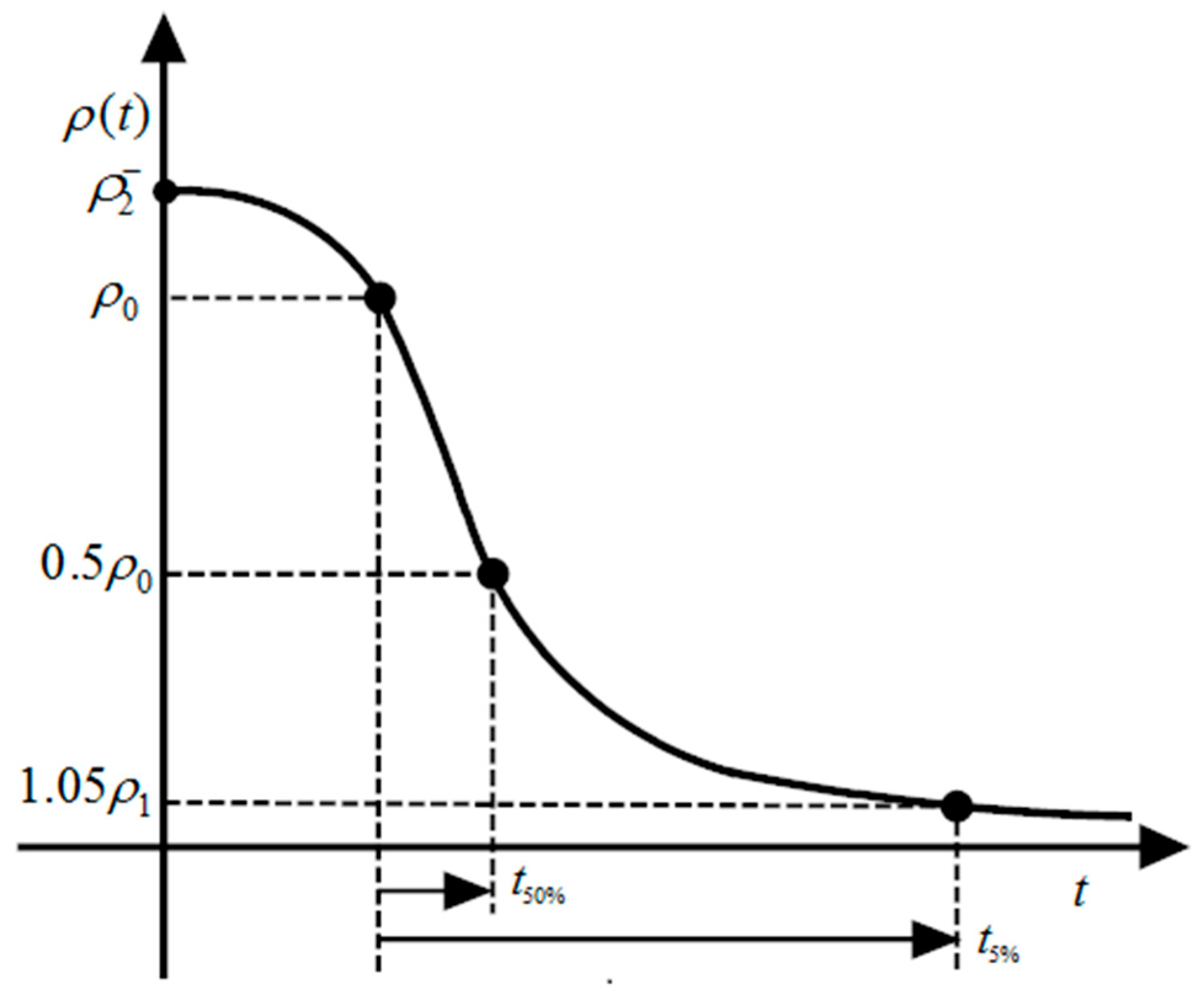
Note that the time constantof the linearized model of the majorant system(36) around the equilibrium pointfor sufficiently largeis.
By integrating the equation with initial condition it is possible to obtain the “half time” and a “settling time” for any shown in Figure 3.
Remark 5.
Note that ifandare independent ofandby using the linearizing control law:
whereis the pseudo-inverse of F, the closed-loop control system (1), (47) becomes:
It is easy to prove that the control system (48) has the following properties:
- (a)
- if
- -
- behavior of a Butterworth filter with angular frequency ;
- -
- time constant ;
- -
- overshoot equal to 4.32%;
- -
- damping ratio ;
- -
- forced responses:
- (b)
- if :
- -
- cutoff angular frequency ;
- -
- max time constant ;
- -
- overshoot 4.32%;
- -
- damping ratio ;
- -
- forced responses:
The proposed control law is also robust with respect to a possible bounded measurement noise on as it is shown by the following theorem.
Theorem 3.
Consider the uncertain nonlinear dynamic system (1), satisfying conditions (1), (2), and controlled with the control law (18). Ifis affected by a bounded measurement noise, the rate ofdue to the noise, for sufficiently largeis inversely proportional to.
Proof.
If is affected by a bounded measurement noise the term must be added to . From (46), for sufficiently large , is inversely proportional to . Hence, the rate of due to the noise , for sufficiently large is inversely proportional to . ☐
Remark 6.
To design the controller it is essential to determine a matrixsatisfying condition (2). Since, in many practical cases, the matrixis the ratio of a multi-affine or quadratic matrix function to a multi-affine or quadratic non-null polynomial with respect to the uncertain parameters and respect to bounded functions, the determination ofcan be easily made by using Lemmas 2, 3 and 4, with:
- (i)
- in the hypothesis thatis a p.d. matrix (in the case of (4) and (9));
- (ii)
- whereis the Jacobian matrix of a suitable coordinate transformation (e.g., the case of robots in their workspace or equipped with cameras used as sensors, in the cases of ships, drones, or satellites);
- (iii)
- ifis independent of(e.g., in the case of kinematic inversion) or, by evaluatingin correspondence of the nominal valueof, in the hypothesis that the variations ofare sufficiently bounded;
- (iv)
- other more suitable matrices(see Application 3).
Remark 7.
After verifying that satisfies the bounding condition of class (2) and determining a matrix satisfying the positivity condition (1), since the tracking error decreases when increases, the single parameter can be determined via simulation or experimentally for an assigned class of references .
Remark 8.
Inequalities used to prove Theorems 1, 2, 3 (especially to prove that when the design parameter a increases the tracking error norm is inversely proportional to) can make very conservative the stated results. A much less conservative estimate of the tracking error norm, i.e., providing smaller values ofand larger values of, by taking into account thatcan be obtained by using the following relation:
that does not use any inequality. The offline use of (51) provides an error much near to the true one, as it turns out to be from Applications 3 and 4, and Examples 2 and 3 in [34].
The determination of the majorant system by using (51) can be easily made by using the Matlab command “fmincon” (which finds a constrained minimum of a function F(X) of several variables and, hence, also a constrained maximum changing the sign to F(X)) and/or by using randomized algorithms (e.g., see [22]).
Note that the current problem is not the computational burden of the controller design, but its simplicity of realization and its effectiveness.
Remark 9.
To reduce the gains of the controller and the control signal, above all during the transient phase, it is possible to:
- 1.
- smooth the trajectories with appropriate filters and suitable initial conditions;
- 2.
- better identify the process parameters and the disturbances, and use a compensation signalto reduce the norm of;
- 3.
- use a connection trajectory if the initial error is excessive [35];
- 4.
- slow down, i.e., replace the reference signalby.
Moreover, consider also the following advantages (see (45) and (46), (49) and (50), Applications 1–4, Example 6 in the Appendix A and [16,19,34,35,38]):
- the control signals are without the chattering phenomenon, since the proposed control law does not present discontinuities and does not have high gains,
- the proposed control laws can be also realized by using simple analogical circuits,
- the stated theoretical results are useful to obtain other analytical and synthetic results, significant both from a theoretical and practical point of view, and to analyze complex systems with parametric and structural uncertainties.
4. Cases Study
The results provided in the preceding section are illustrated through some interesting applications.
Application 1.
Consider the electronic circuit in Figure 4. In the hypothesis that the considered transistor is a BJT described by the equations:
A goal is to determine the working point i.e., the solution of the nonlinear equations system:
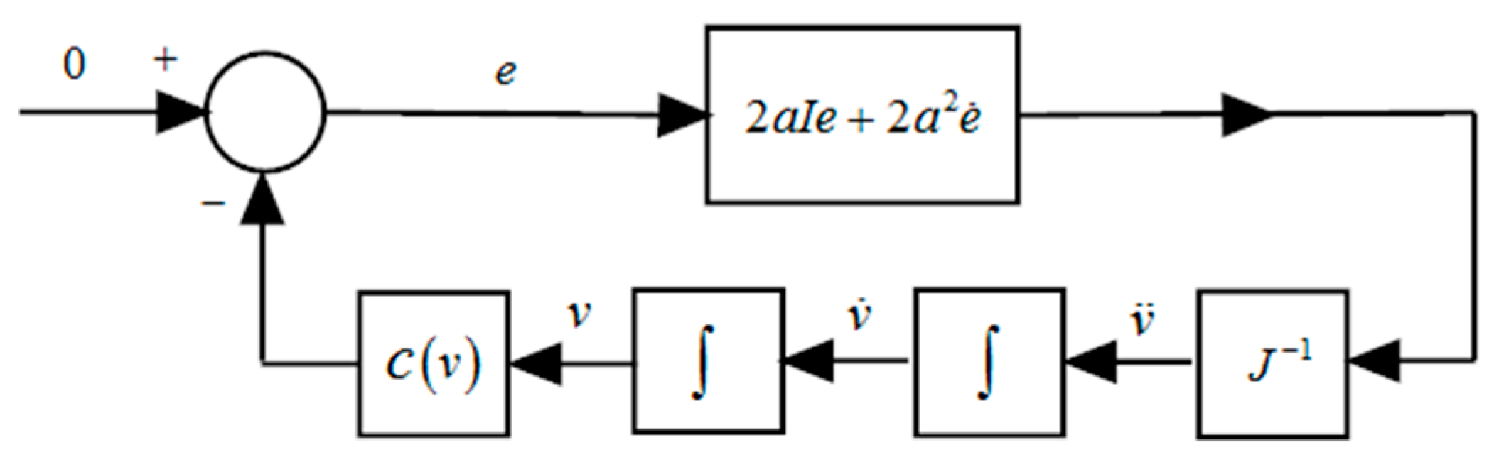
Based on (17) and Theorems 1 and 2 the value of can be obtained by integrating the control scheme in Figure 5.
Under the following hypotheses:
by numerically computing the Jacobian matrix as follows:
with , and by using the Matlab solver ode45 with variable-step, after 1.2 s the results reported in Table 1 are obtained.
Application 2.
Consider the planar robot in Figure 6.
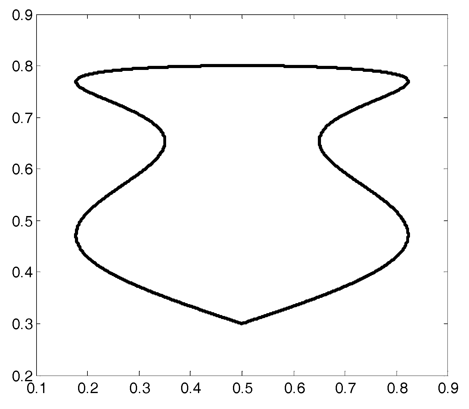
The goal is to realize the object in Figure 7 with the following time histories in the workspace:
The time history of the trajectory in the joint space can be obtained by integrating the control scheme in Figure 8, much easier than the ones proposed in ([10,11,13,33] and the related references therein), where:
the value of can be determined by using the method presented in Application 1 and the value of with the relation
Note that slowing down , i.e., replacing the reference signal by the value of the error norm of function (17), for , is reduced of and, hence, for sufficiently large , also the error norm is reduced of .
In the hypothesis that by choosing and by using the Matlab solver ode4 with fixed-step , the results shown in Figure 9, Figure 10 and Figure 11 are obtained.
In Figure 12 the accelerations are reported by numerically deriving and the related errors.
Remark 10.
To obtain the kinematic inversion, instead of starting from the “exact” initial conditions, it is possible to extend to left(see Figure 13) and to start from initial conditions also very different from the “exact” one.
The following applications show how it is easy to design, by using the proposed method, simple, robust and efficient controllers, without chattering, with respect to other methods available in the literature.
Application 3.
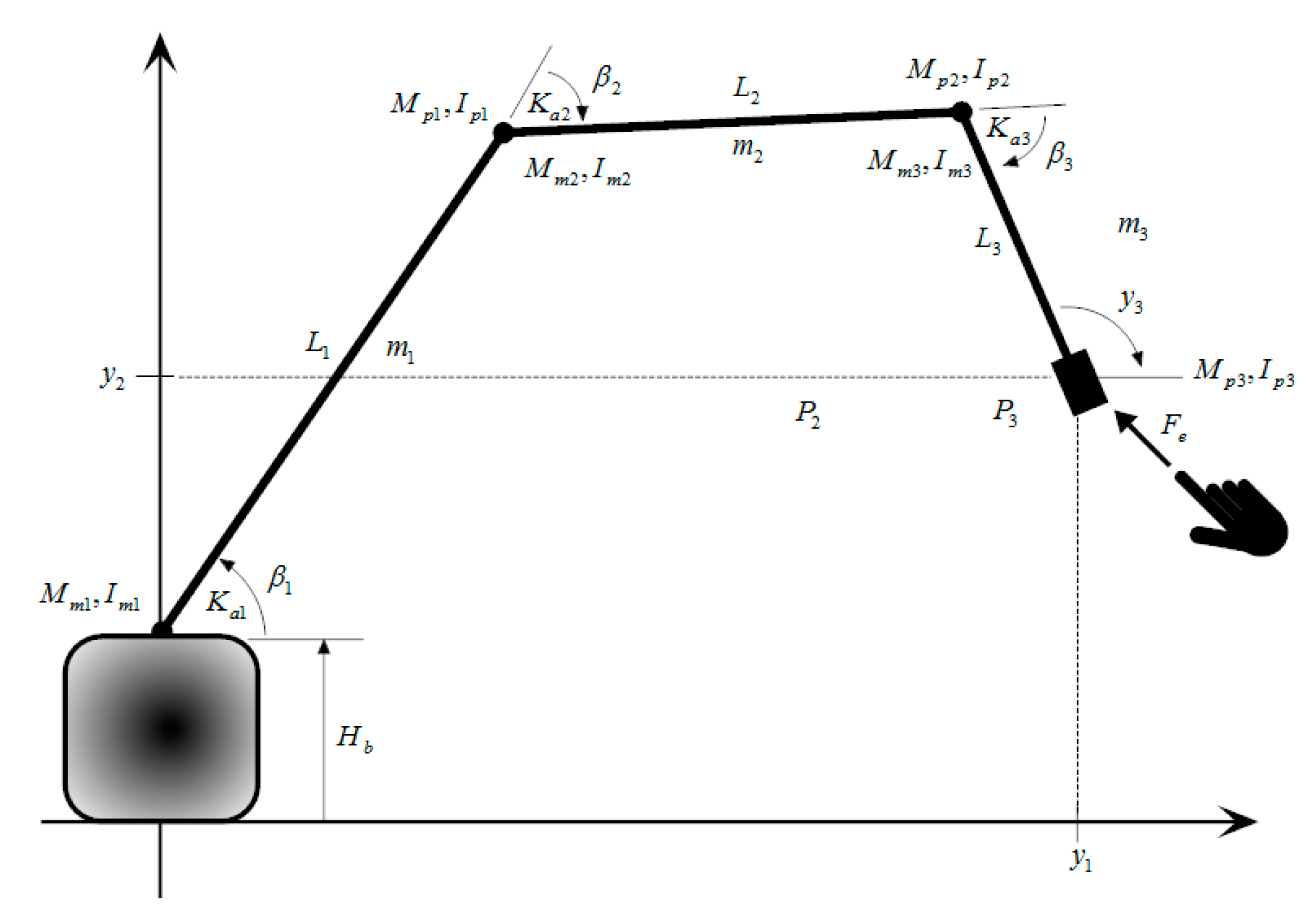
In this application, the design of some robust controllers is considered for a three-link planar robot (see Figure 14). The goal is to perform assembly and/or warehouse tasks with any human operator (see Supplementary Material too).
Suppose, for simplicity, that the i-th link of the robot is a straight line of constant section and a mass density with the tip two masses and of inertia moments and If:
then the inertia matrix can be computed by using the following relations (see [9]):
where the matrices (and the corresponding model of the robot) can be found using the algorithm from [9].
The Jacobian matrix is computed as:
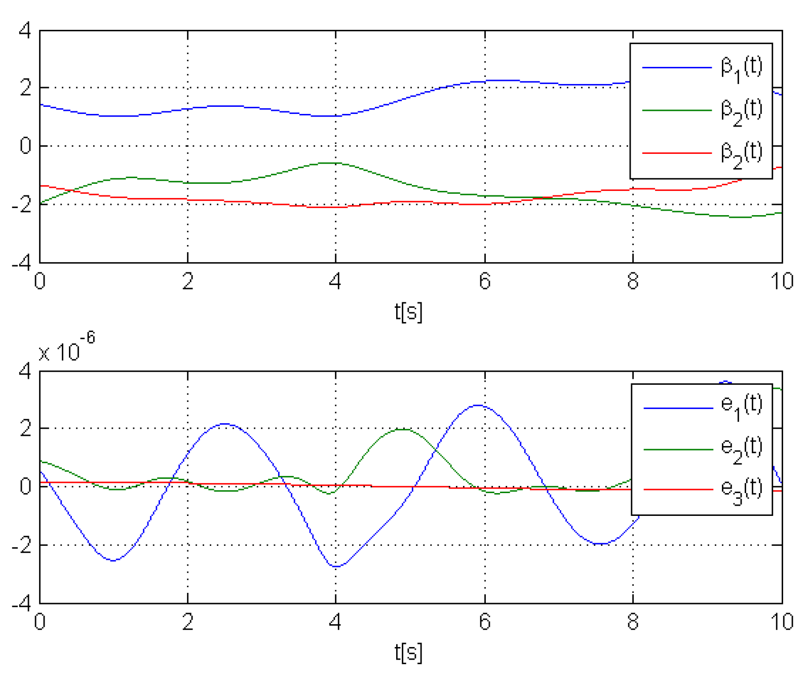
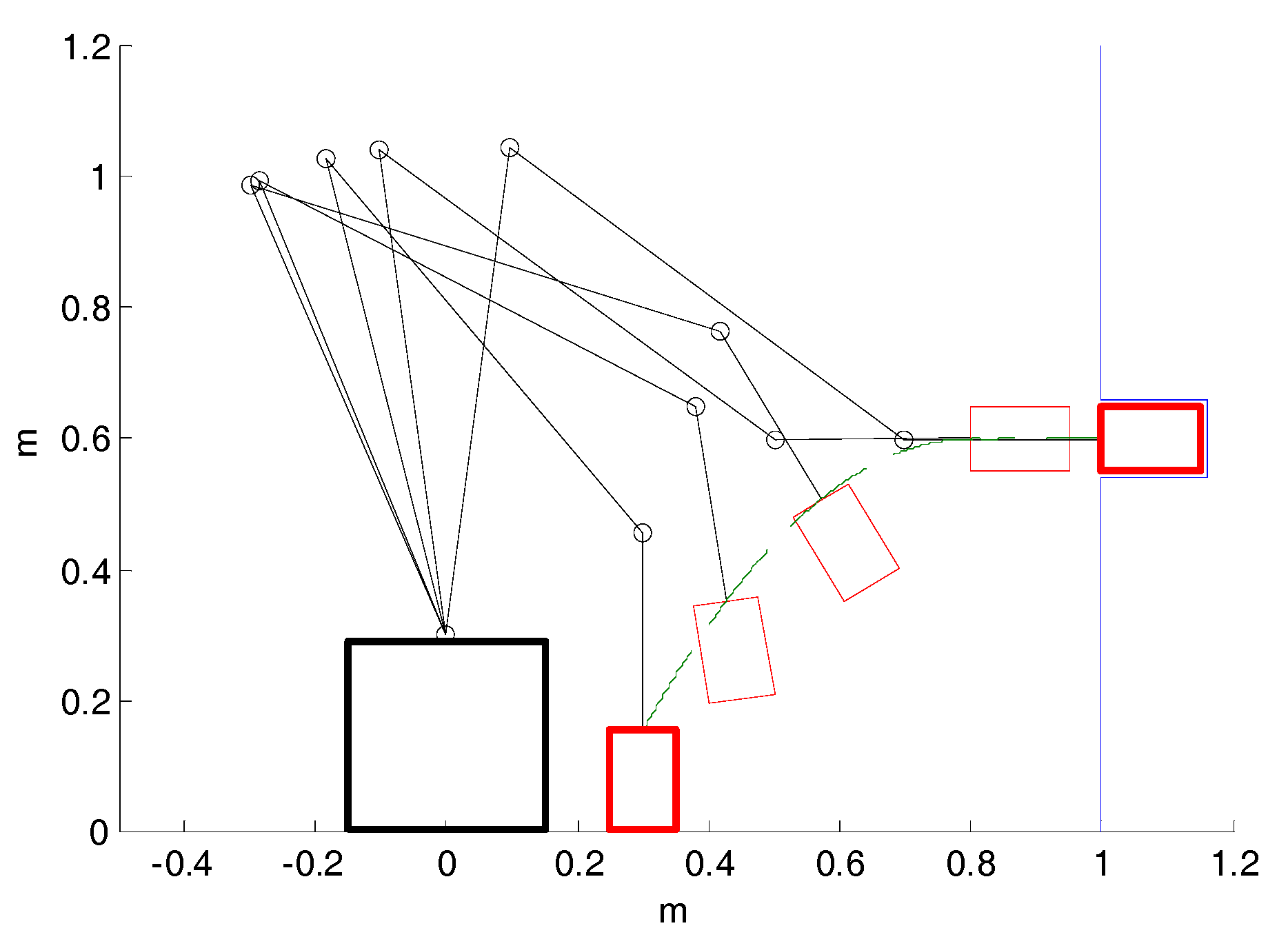
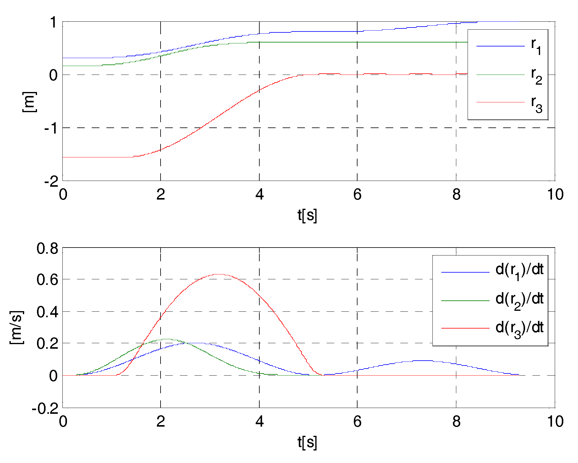
(A) Suppose that the goal is to perform the assembly or warehouse task shown in Figure 15, with behaviors of and of , in the workspace, reported in Figure 16. In Figure 17 the corresponding behaviors in the joint space are reported. These ones are obtained from the original behaviors by using a third-order Bessel filter with and the kinematic inversion.
(a) Using Lemmas 2 and 4, a matrix of the type which satisfies condition , , is:
(b) By using Lemmas 2 and 4, a matrix of the type which satisfies the condition , , is:
(c) By using Lemmas 2 and 4, a matrix of the type which satisfies the condition , and , , is:
(d) By using Lemmas 2 and 4, a matrix of the type which satisfies the condition , , and , is:
(e) Finally, by using Lemmas 2 and 4, it can be easily verified that the constant matrix:
satisfies the condition , and , where:
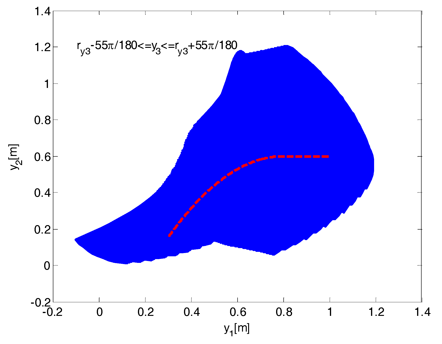
In Figure 18 the neighborhood of in the workspace, corresponding to the neighborhoods of , is shown.
Suppose that .
(A1) If the following a simple control law (three classic PD controllers in the joint space) is used:
The graphical model of the majorant system , obtained with (51), is reported in Figure 19.
From Figure 19, in accordance with Theorem 2, it is:
- if , then ;
- if , then (e.g., if , at less ,
In Figure 20 and Figure 21, the behaviors of are shown in the hypothesis of From Figure 21 it is ; this value is very close to the computed one 0.00362.
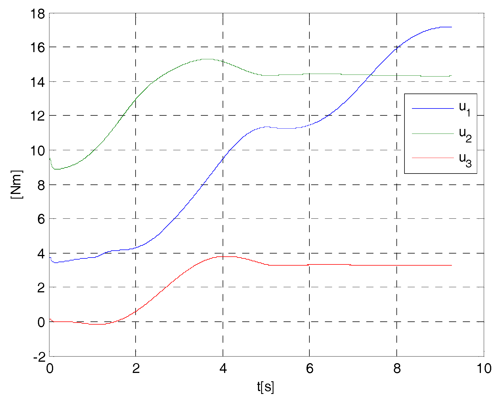
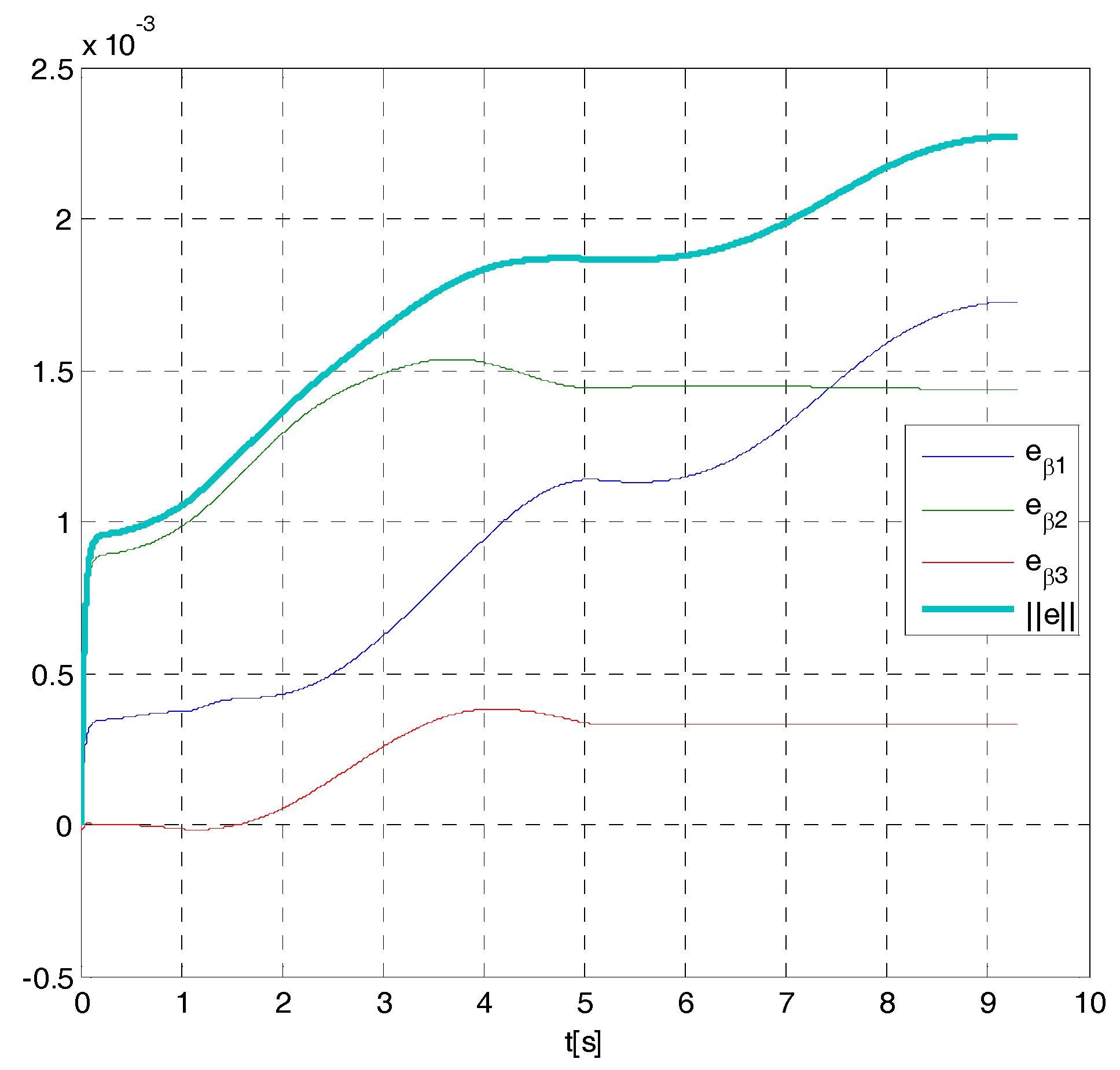
(A3) With the control law:
where are the gravity torques, with , the errors are shown in Figure 23; while with the errors, as shown in Figure 24, are approximately 4 times larger, in accordance with (46).
If the velocity is affected by a measurement noise uniformly distributed in , always with the controller (70) with , the errors are shown in Figure 25, in accordance with Theorem 3.
Now consider the control in the workspace.
(A4) With the control law:
where are the gravity torques, the errors are shown in Figure 26.
(A5) With the control law:
where are the gravity torques, the errors are shown in Figure 27.
(A6) Finally, by using the simple control law:
the errors are shown in Figure 28.
Remark 11.
Note that the control law (73) is independent of.
(B) Now consider the interaction of the considered robot with a human operator. If is the generalized force exerted by the operator on the end-effector of the robot, the model is:
Instead of opposing the action of , this action can be supported by controlling the robot such to behave as an impedance, comparable to a generalized mass-spring-damper system.
The above control can be achieved using the impedance control scheme in Figure 29.
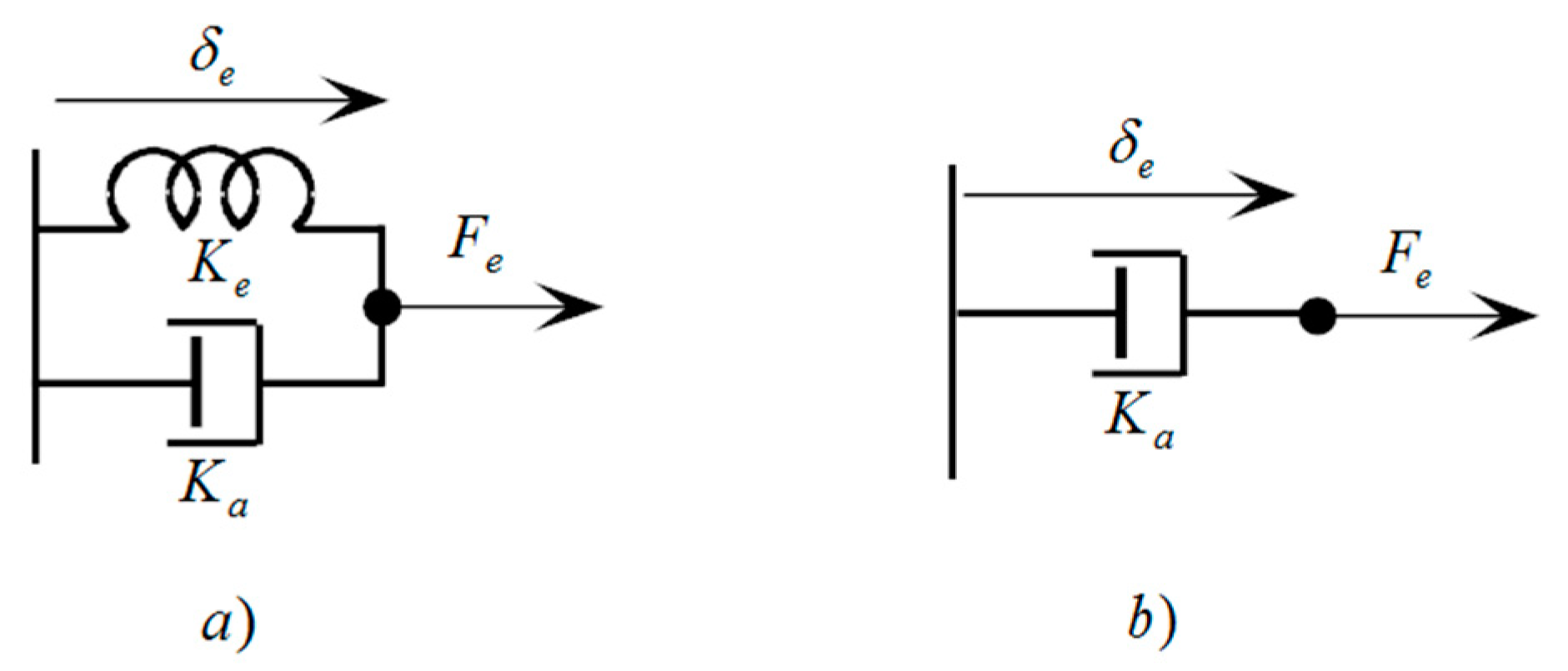
(B1) If the considered impedance is the one of a spring-damper system (see Figure 30a), then the model is:
Note that the output can be used to realize the derivative action of the PD controller if is measurable.
In the hypothesis that , , where is the third-order identity matrix, the used controller is (73), with , assuming that the behaviors of the forces are as shown in Figure 31 and the behaviors of are as shown in Figure 32, then the behaviors of are reported in Figure 32.
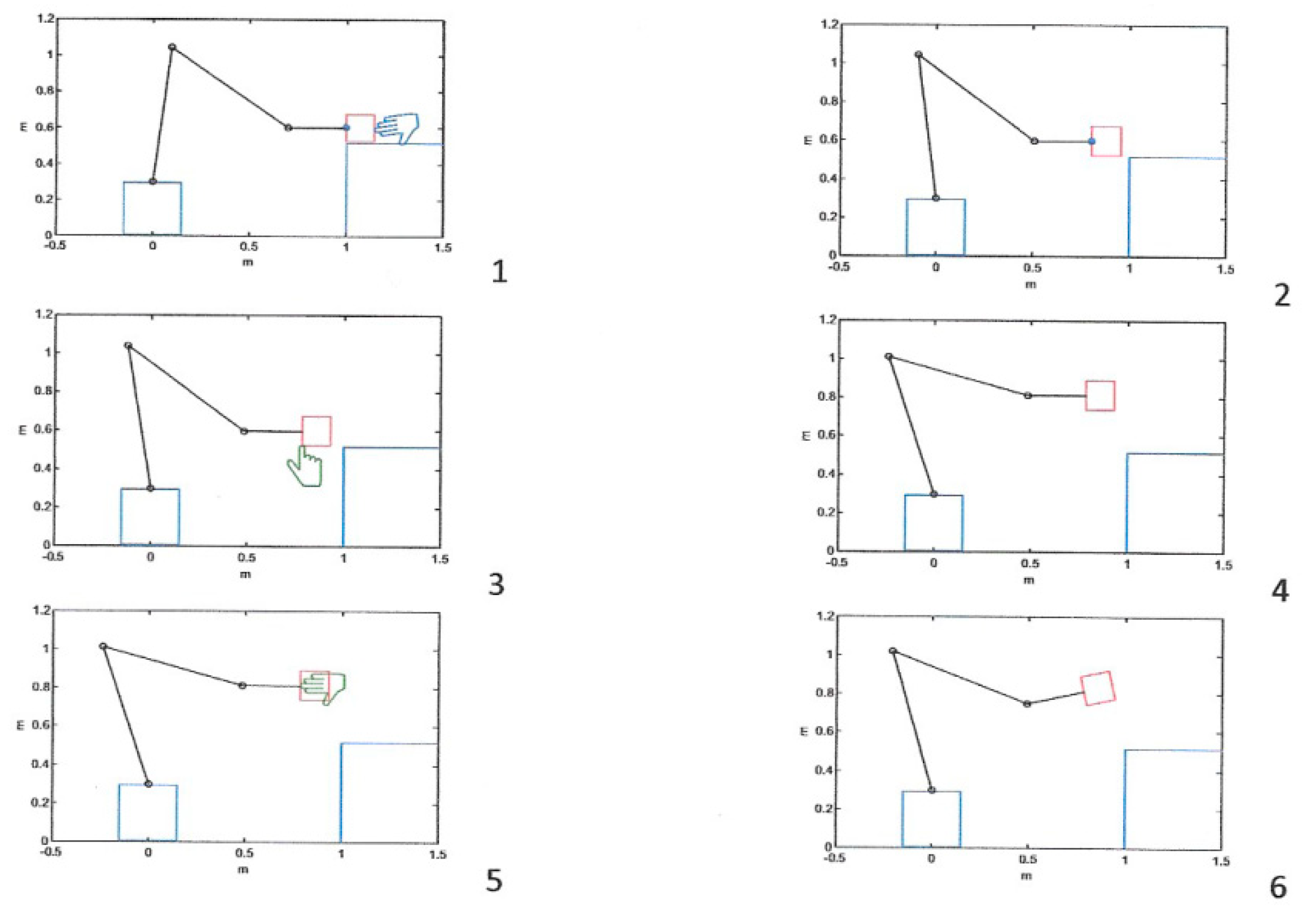
In Figure 33, selected phases of the robot interaction with a human operator are reported assuming that the impedance is as shown in Figure 30a).
(B2) If the considered impedance is the impedance of a damper (see Figure 30b), then the model is:
In the hypothesis that , where is the third-order identity matrix, the used controller is (73) with , assuming that the behaviors of are as shown in Figure 34 and the behaviors of the forces are as shown in Figure 31, then the behaviors of are reported in Figure 34.
In Figure 35, selected phases of the interaction are reported in the hypothesis of an impedance as in Figure 30b.
Application 4.
To be further convinced of the usefulness of the developed theory, many other examples can be provided.
This example considers the plant:
that does not belong to the class of system (9).
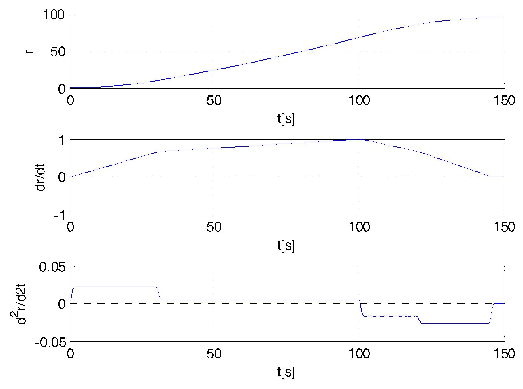
The desired reference signal is the one shown in Figure 36, which is obtained from an easily generable piecewise-linear signal filtered by using a third-order Bessel filter with .
The following PD controller is applied:
with G = 3, satisfying condition (2).
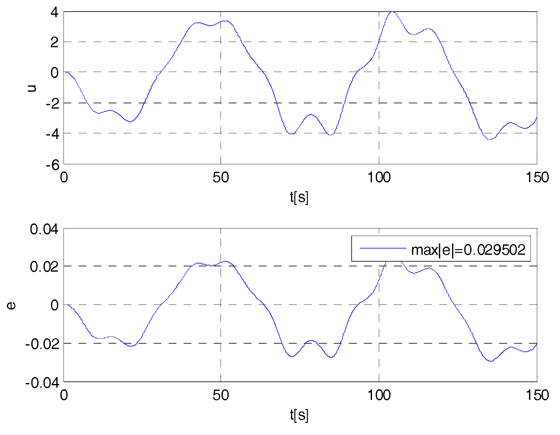
In Figure 37, the graphical models of the majorant systems obtained with (78) are reported for .
Note that , , in accordance with the fact that, for sufficiently large , the maximum of is inversely proportional to .
Remark 12.
By taking into account numerous significant simulations made by the author, it follows that the control system performance is still good if the derivative action is a real one with time constantand/or if the used actuator is a real one with electrical time constant(see Example A3 in the Appendix A). This can be explained by taking into account Remark 5, Theorem 3 and the robustness of the proposed control law with respect to parametric uncertainties. The proof of the robustness of the control system with respect towill be the subject of a future paper.
5. Conclusions and Future Developments
In this paper, for a broad class of uncertain nonlinear MIMO systems, including many manufacturing systems and land, sea, and air transportation systems, a novel and unified robust control approach has been provided. It allows to design robust PD-type control laws without chattering to track a reference signal with bounded second derivative with the tracking error norm smaller than a prescribed value, despite the presence of bounded disturbances, parametric, and structural uncertainties, and bounded measurement noises. It has also been proved that the proposed control laws are robust with respect to bounded measurement noises.
With reference to the mechanical and transportation systems, this theory has been successfully applied when the controller uses information signals related to the joint space or signals related to the workspace. Moreover, the proposed results have also been fruitfully used for the control of human-machine interaction.
The obtained theoretical results have been illustrated through four relevant theoretical and engineering applications.
The main advantages of the results of this study can be summarized as follows:
- The considered class of nonlinear uncertain MIMO systems is broad and includes an important class of uncertain linear systems.
- A comprehensive approach based on the concept of majorant systems is provided to design smooth robust controllers. They have been used to track a generic reference signal with bounded second derivative with a tracking error norm smaller than a prescribed value.
- The obtained control laws are easy to design and implement. These laws have no high gains and are free from discontinuities.
- Suitable filtering laws are proposed for tracked trajectories to facilitate the implementation of the control laws and reduce the control magnitude, particularly during the transient phase.
- The maximum tracking error can be fixed a priori despite bounded parametric uncertainties, disturbances, and velocity measurement noise.
- A simple relation exists between a single design parameter of the controller and the maximum tracking error, which is useful for obtaining the desired tracking precision.
- The proposed control laws are robust with respect to bounded measurement noises.
The established theoretical results can be used also to obtain further analysis and synthesis results and study complex systems with parametric and structural uncertainties. Moreover, other engineering and/or theoretical complex nonlinear uncertain systems can be easily controlled as the treated case studies, e.g., a drone and missile in the ongoing activity of the author.
Future developments of this methodology and ongoing work of the author are: the theoretical extension of the proposed results when real derivative actions, real actuators and real amplifiers based on the PWM technique are considered.
Supplementary Materials
The following are available online at https://www.mdpi.com/2076-3417/8/11/2236/s1, An illustrative video of the robotic assembly system reported in Application 3 is provided. This video shows: (1) an operation of robotic assembly; (2) a human-robot interaction of spring-damper type; (3) a human-robot interaction of damper type.
Funding
This work was supported by the Italian Ministry of Education, Universities and Research.
Acknowledgments
The author is deeply grateful to Professor G. Celentano, Senior Member of Automation group of the Department of Electrical Engineering and Information Technology, University of Naples Federico II, for his valuable encouragement and advice.
Conflicts of Interest
The author declares no conflict of interest.
Appendix A
In the following six easy examples are provided. The first five ones clearly show how numerous control techniques available in the literature for significant classes of linear and nonlinear systems can produce unstable control system or can significantly reduce the performance of the control system, under the following realistic hypotheses:
- (1)
- parametric uncertainties;
- (2)
- real actuators;
- (3)
- measurement noise;
- (4)
- finite online computation time of the control signal.
The sixth example shows that the above mentioned disadvantages can be eliminated or reduced with the results proposed in the paper.
Example A1.
Consider the position control of an AGV. A model of the simple AGV in Figure A1 is:
Figure A1.
AGV.

Suppose the slope of the road constant and unknown. Including the gravity action in d, in the hypothesis that and the model is represented as:
By using the control law:
based on the inverse dynamic control technique, the closed-loop control system turns out to be:
If the dynamical model of the tracking error (A4) is:
For and in the presence of any disturbance with bounded derivative, applying the method proposed in [34,35], the tracking error is , where .
For , instead, the tracking error is not acceptable since system (A4) is unstable.
Therefore, the inverse dynamic control technique, under the hypothesis of parametric uncertainties, is not reliable!
Example A2.
Suppose that,and that the slope of the road is such that. In this case the model is:
By using the control law:
based on the feedback linearization technique, the dynamical model of the tracking error is:
For and , in the presence of any bounded disturbance , applying the method proposed in [34,35], the tracking error of any reference with bounded second derivative is , where .
Instead, for the tracking error is not always acceptable, since system (A1) can be unstable for .
Hence, the control method based on the feedback linearization technique, under the hypothesis of parametric uncertainties, is not always reliable, especially for robots!
Example A3.
Consider the system (A2) for:
If , i.e., under the hypothesis of an almost ideal actuator, then and, hence, for , it is:
By using the control law:
the dynamical model of the tracking error, in the hypothesis that is:
For and , applying the first of (49), it is .
From (A9), (A11) and (A13) the exact model turns out to be:
from which, by setting , it is:
It is easy to verify that for , the control system is unstable, while for , the control system is stable (see Figure A2). For , it is: , i.e., if the time constant of the actuator is equal to in the hypothesis of real actuator (A11), the dynamic matrix A has a couple of dominant eigenvalues equal to the poles of the closed-loop system (A14).
Figure A2.
Stability and instability regions (in red lower and upper bounds of separation between the two regions).
Figure A2.
Stability and instability regions (in red lower and upper bounds of separation between the two regions).

Hence, it can be said that the control techniques of the mechanical systems, especially for robots, which make the hypothesis of ideal actuators (torque and/or force actuators), are not reliable!
Example A4.
Consider the system (A2):
To control the system (A17) with the MPC technique (e.g., [37,43]), consider the following system as the nominal model in order to predict its evolution:
Fixed the sampling time , let:
be the discrete time models of the systems (A18) and (A19), respectively.
Said the reference signal to track, it is:
As control consider the one minimizing the performance index:
Suppose that:
Figure A3.
Time histories of u, r, y with the model predictive control (MPC) controller.

If the velocity is affected by a measurement noise uniformly distributed in the interval , some time histories of u, r and y are reported in Figure A4 and Figure A5.
Figure A4.
Time histories of u, r, and y with the MPC controller in the hypothesis of measurement noise on .
Figure A4.
Time histories of u, r, and y with the MPC controller in the hypothesis of measurement noise on .

Figure A5.
Time histories of u, r, y with an MPC controller in the hypothesis of measurement noise on .
Figure A5.
Time histories of u, r, y with an MPC controller in the hypothesis of measurement noise on .

From Figure A4 and Figure A5 it clearly emerges that in general an MPC controller is very sensitive to measurement errors.
Moreover, by noting that:
- (1)
- for more complex nonlinear systems with parametric uncertainties the MPC controller requires a high online computational burden,
- (2)
- in general, the properties of asymptotic stability depend in a complex way on the model chosen to predict the evolution and on other parameters of the controller,
it can be deduced that, in many cases, controllers based on other control techniques should be preferred with respect MPC.
Example A5.
Consider the system:
In the hypothesis that:
consider the control law:
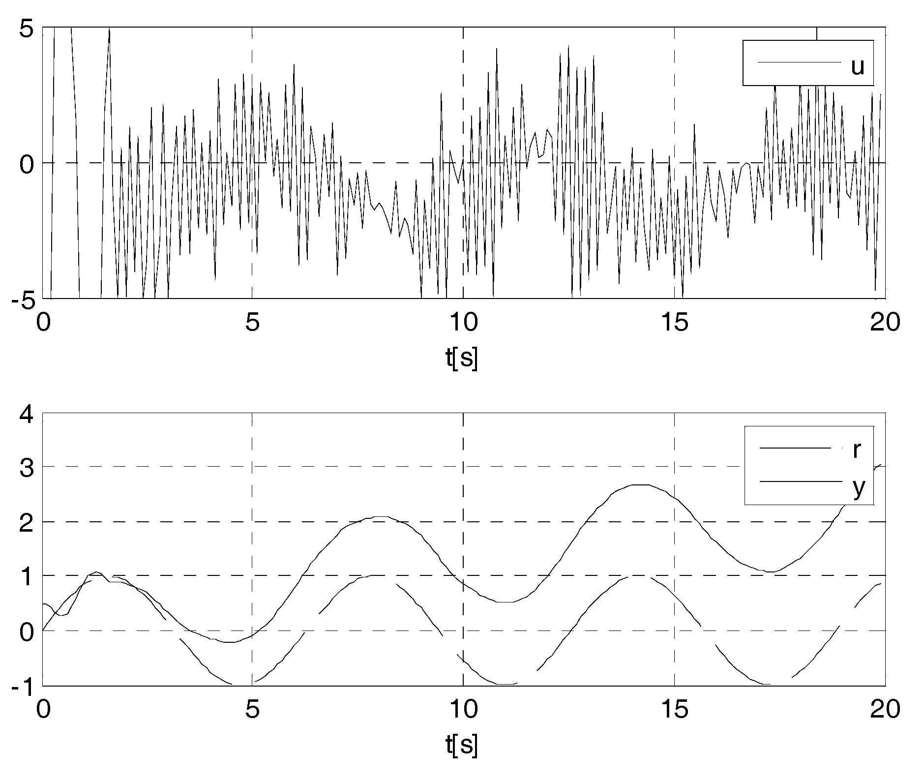
In Figure A6 and Figure A7, the time histories of are reported in the hypothesis that and that downstream of the controller there is a zero holder hold (ZOH) with sampling time respectively.
Figure A6.
Time histories of with a chattering control law and sampling time of the zero holder hold (ZOH) hold .
Figure A6.
Time histories of with a chattering control law and sampling time of the zero holder hold (ZOH) hold .

Figure A7.
Time histories of with a chattering control law and sampling time of the ZOH hold .

From Figure A6 and Figure A7 it can be deduced that the chattering control law with finite switching frequency does not provide good performance, especially of the error derivative .
Under the hypothesis of real actuators and real derivative actions, the control system can be even unstable.
Example A6.
Still, consider the system (A25) with d and r in (A26).
By using the simple control law:
designed with the proposed methodology, in the hypothesis that and that downstream of the controller there is a pulse-width modulation (PWM) modulator with sampling time the time histories of are reported in Figure A8 and Figure A9, respectively.
Figure A8.
Time histories of with the proportional-derivative (PD) controller (A3) and a PWM modulator with sampling time .
Figure A8.
Time histories of with the proportional-derivative (PD) controller (A3) and a PWM modulator with sampling time .

Figure A9.
Time histories of with the PD controller (A3) and a PWM modulator with sampling time .

From Figure A8 and Figure A9 and from the corresponding Figure A6 and Figure A7 it emerges how the performance of the control system with a controller designed by using the stated theory and implemented by using a PWM modulator are better, both regarding to the amplitude of the control signal (see Figure A1, as well) and the precision, than the performance obtained with a controller designed with the control techniques using high frequency and high-amplitude control signals (e.g., [4,10,14,31,40,41] and related references therein) and implemented with commutation devices with evaluation of the sign at finite frequency.
Moreover, it is worth noting that the PWM modulator technology is at low cost and very used in the engineering practice.
Finally, take also into account:
- (1)
- (2)
- that the articulated mechanical systems are very complex (see [6]) and that, hence, techniques using their online models are difficult to be implemented without delays; therefore, the delays due to the online computation times can make unstable the control system.
Thus, it clearly emerges that the results proposed in this paper (see also Applications 1–4), which are a broad generalization of the technique presented in [21], are very useful from a theoretical and applicative point of view.

References
- Dorato, P. (Ed.) Robust Control; IEEE Press: New York, NY, USA, 1987. [Google Scholar]
- Abdallah, C.T.; Dawson, D.; Dorato, P.; Jamshidi, M. Survey of robust control for rigid robots. IEEE Control Syst. 1991, 11, 24–30. [Google Scholar] [Green Version]
- Ackermann, J. Robust Control: Systems with Uncertain Physical Parameters; Springer: New York, NY, USA, 1993. [Google Scholar]
- Jafarov, E.M.; Tasaltin, R. Robust sliding-mode control for the uncertain MIMO aircraft model F-18. IEEE Trans. Aerosp. Electron. Syst. 2000, 36, 1127–1141. [Google Scholar]
- Adams, R.J.; Buffington, J.M.; Sparks, A.G.; Banda, S.S. Robust Multivariable Flight Control; Springer: London, UK, 1994. [Google Scholar]
- Wu, C.-J.; Huang, C.-H. A neural network controller with PID compensation for trajectory tracking of robotic manipulators. J. Frankl. Inst. 1996, 333, 523–537. [Google Scholar] [CrossRef]
- Yoshikawa, T. Force Control—Foundations of Robotics: Analysis and Control; The MIT Press: Cambridge, MA, USA, 2003. [Google Scholar]
- Tsuji, T.; Tanaka, Y. Tracking control properties of human-robotic systems based on impedance control. IEEE Trans. Syst. Man Cybern. A 2005, 35, 523–535. [Google Scholar] [CrossRef]
- Celentano, L.; Iervolino, R. New results on robot modeling and simulation. ASME J. Dyn. Syst. Meas. Control 2006, 128, 128–811. [Google Scholar] [CrossRef]
- Chung, W.; Fu, L.-C.; Hsu, S.-H. Motion control. In Springer Handbook of Robotics; Siciliano, B., Khatib, O., Eds.; Springer: Berlin, Germany, 2008. [Google Scholar]
- Spong, M.W.; Hutchinson, S.; Vidyasagar, M. Robot. Modeling and Control; John Wiley & Sons, Inc.: New York, NY, USA, 2006. [Google Scholar]
- Chang, Y.-C.; Yen, H.-M. Robust tracking control for a class of uncertain electrically driven robots. IET Control Theory Appl. 2009, 3, 519–532. [Google Scholar] [CrossRef]
- Siciliano, B.; Sciavicco, L.; Villani, L.; Oriolo, G. Robotics: Modelling, Planning and Control; Springer: London, UK, 2009. [Google Scholar]
- Utkin, V.; Guldner, J.; Shi, J. Sliding Mode Control in Electro-Mechanical Systems; CRC Press: Boca Raton, FL, USA, 2009. [Google Scholar]
- Sabanovic, A.; Ohnishi, K. Motion Control Systems, Chapters: Interactions in Operational Space and Interactions and Constraints; Wiley-IEEE Press: Hoboken, NJ, USA, 2011. [Google Scholar]
- Celentano, L.; Coppola, A. A wavelet based method to modeling realistic flexible robots. In Proceedings of the 18th IFAC World Congress, Milano, Italy, 28 August–2 September 2011; pp. 929–937. [Google Scholar]
- Tamura, K.; Ohmori, H. Adaptive PID control for asymptotic tracking problem of MIMO systems. In PID Control, Implementation and Tuning; Mansour, T., Ed.; InTech Educ.: London, UK, 2011; pp. 187–200. [Google Scholar]
- Celentano, L. Robust Tracking Controllers Design with Generic References for Continuous and Discrete Uncertain Linear SISO Systems; LAP LAMBERT Academic Publishing: Saarbrücken, Germany, 2012. [Google Scholar]
- Celentano, L. An innovative method to modeling realistic flexible robots. Appl. Math. Sci. 2012, 6, 3623–3659. [Google Scholar]
- Piltan, F.; Yarmahmoudi, M.H.; Shamsodini, V.; Mazlomian, E.; Hosainpour, A. PUMA-560 Robot Manipulator Position Computed Torque Control Methods Using MATLAB/SIMULINK and Their Integration into Graduate Nonlinear Control and MATLAB Courses. Int. J. Robot. Autom. 2012, 3, 167–191. [Google Scholar]
- Celentano, L. Robust tracking method for uncertain MIMO systems of realistic trajectories. J. Frankl. Inst. 2013, 350, 437–451. [Google Scholar] [CrossRef]
- Tempo, R.; Calafiore, G.; Dabbene, F. Randomized Algorithms for Analysis and Control of Uncertain Systems: With Applications, 2nd ed.; Springer: London, UK, 2013. [Google Scholar]
- Liu, H.; Xi, J.; Zhong, Y. Robust motion of quadrotors. J. Frankl. Inst. 2014, 351, 5494–5510. [Google Scholar] [CrossRef]
- Leban, F.A.; Díaz-Gonzalez, J.; Parker, G.G.; Zhao, W. Inverse kinematic control of a dual crane system experiencing base motion. IEEE Trans. Control Syst. Technol. 2015, 23, 331–339. [Google Scholar] [CrossRef]
- Jang, J.T.; Gong, H.C.; Lyou, J. Computed torque control of an aerospace craft using nonlinear inverse model and rotation matrix. In Proceedings of the 15th International Conference on Control, Automation and Systems (ICCAS), Busan, Korea, 13–16 October 2015; pp. 1743–1746. [Google Scholar]
- Rastogi, E.; Prasad, L.B. Comparative performance analysis of PD/PID computed torque control, filtered error approximation based control and NN control for a robot manipulator. In Proceedings of the 2015 IEEE UP Section Conference on Electrical Computer and Electronics (UPCON), Allahabad, India, 4–6 December 2015; pp. 1–6. [Google Scholar]
- Zhou, Y.; Chen, M.; Jiang, C. Robust tracking control of uncertain MIMO nonlinear systems with application to UAVs. IEEE/CAA J. Autom. Sin. 2015, 2, 25–32. [Google Scholar]
- Labrecque, P.D.; Haché, J.-M.; Abdallah, M.; Gosselin, C. Low-Impedance Physical Human Robot Interaction Using an Active–Passive Dynamics Decoupling. IEEE Robot. Autom. Lett. 2016, 1, 938–945. [Google Scholar] [CrossRef]
- Yoon, Y.; Sun, Z. Robust motion control for tracking time-varying reference signals and its application to a camless engine valve actuator. IEEE Trans. Ind. Electron. 2016, 63, 5724–5732. [Google Scholar] [CrossRef]
- Xiao, B.; Yang, J.; Fu, Z.; Wu, C.; Huo, X. A proportional-derivative-type attitude tracking control of satellite. In Proceedings of the 35th Chinese Control Conference (CCC), Chengdu, China, 27–29 July 2016; pp. 10858–10863. [Google Scholar]
- Li, P.; Ma, J.; Zheng, Z. Robust adaptive sliding mode control for uncertain nonlinear MIMO system with guaranteed steady state tracking error bounds. J. Frankl. Inst. 2016, 353, 303–321. [Google Scholar] [CrossRef]
- Kumar, V.; Rana, K.P.S.; Mishra, P. Robust speed control of hybrid electric vehicle using fractional order fuzzy PD and PI controllers in cascade control loop. J. Frankl. Inst. 2016, 353, 1713–1741. [Google Scholar] [CrossRef]
- Brahmi, B.; Saad, M.; Rahman, M.H.; Ochoa-Luna, C. Cartesian trajectory tracking of a 7-dof exoskeleton robot based on human inverse kinematics. IEEE Trans. Syst. Man Cybern. Syst. 2017, 99, 1–12. [Google Scholar] [CrossRef]
- Celentano, L. Design of a pseudo-PD or PI robust controller to track C2 trajectories for a class of uncertain nonlinear MIMO system. J. Frankl. Inst. 2017, 354, 5026–5055. [Google Scholar] [CrossRef]
- Celentano, L. Pseudo-PID robust tracking method for a class of mechanical uncertain MIMO systems. In Proceedings of the 20th IFAC World Congress, Toulouse, France, 9–14 July 2017; Volume 50, pp. 1545–1552. [Google Scholar]
- Wang, H.; Shi, P.; Li, H.; Zhou, Q. Adaptive Neural Tracking Control for a Class of Nonlinear Systems with Dynamic Uncertainties. IEEE Trans. Cybern. 2017, 47, 3075–3087. [Google Scholar] [CrossRef] [PubMed]
- Sun, Z.; Xia, Y.; Dai, L.; Liu, K.; Ma, D. Disturbance Rejection MPC for Tracking of Wheeled Mobile Robot. IEEE/ASME Trans. Mechatron. 2017, 22, 2576–2587. [Google Scholar] [CrossRef]
- Celentano, L.; Basin, M. An Approach to Design Robust Tracking Controllers for Nonlinear Uncertain Systems. IEEE Trans. Syst. Man Cybern. Syst. 2018, in press. [Google Scholar] [CrossRef]
- Ha, W.; Back, J. A disturbance observer-based robust tracking controller for uncertain robot manipulators. Int. J. Control Autom. Syst. 2018, 16, 417–425. [Google Scholar] [CrossRef]
- Chen, L.-H.; Peng, C.-C. Extended backstepping sliding controller design for chattering attenuation and its application for servo motor control. Appl. Sci. 2017, 7, 220. [Google Scholar] [CrossRef]
- Wu, K.; Cai, Z.; Zhao, J.; Wang, Y. Target tracking based on a nonsingular fast terminal sliding mode guidance law by fixed-wing UAV. Appl. Sci. 2017, 7, 333. [Google Scholar] [CrossRef]
- Guo, Q.; Liu, Y.; Jiang, D.; Wang, Q.; Xiong, W.; Liu, J.; Li, X. Prescribed performance constraint regulation of electrohydraulic control based on backstepping with dynamic surface. Appl. Sci. 2018, 8, 76. [Google Scholar] [CrossRef]
- Wang, C.; Liu, X.; Yang, X.; Hu, F.; Jiang, A.; Yang, C. Trajectory tracking of an omni-directional wheeled mobile robot using a model predictive control strategy. Appl. Sci. 2018, 8, 231. [Google Scholar] [CrossRef]
- Celentano, L.; Basin, M. New results on robust stability analysis and synthesis for MIMO uncertain systems. IET Control Theory Appl. 2018, 12, 1421–1430. [Google Scholar] [CrossRef]
Figure 1.
Illustration of the bounding condition for f of class

Figure 2.
Illustration of .

Figure 3.
Illustration of the times and .

Figure 4.
The considered electronic circuit.

Figure 5.
Control scheme to determine .

Figure 6.
The considered planar robot.

Figure 7.
Object to be realized.

Figure 8.
Control scheme for the kinematic inversion.

Figure 9.
The trajectory and the related error

Figure 10.
The velocity and the related error

Figure 11.
The acceleration and the related error .

Figure 12.
The acceleration obtained by numerically deriving and the related error .

Figure 13.
Extension to left of the reference.

Figure 14.
Considered planar robot.

Figure 15.
Desired operation (the motion of the payload is in red).

Figure 16.
Time histories of and in the workspace.

Figure 17.
Time histories of and in the joint space.

Figure 18.
Neighborhood (blue) of (red).

Figure 19.
Function and time histories of of the majorant system with the controller in (68).


Figure 20.
Time histories of the control torques with the controller (68).

Figure 21.
Time histories of the errors with the controller (68).

Figure 22.
Time histories of the errors with the controller (69).

Figure 23.
Time histories of the errors using the controller (70) with .

Figure 24.
Time histories of the errors using the controller (70) with .

Figure 25.
Time histories of using the controller (70) with .

Figure 26.
Time histories of the errors with the controller (71).

Figure 27.
Time histories of the errors with the controller (72).

Figure 28.
Time histories of the errors using the controller (73).

Figure 29.
Impedance control scheme.

Figure 30.
Virtual impedances: (a) spring-damper, (b) damper.

Figure 31.
Behaviors of the forces

Figure 32.
Behaviors of and of assuming that the impedance is as shown in Figure 30a).
Figure 32.
Behaviors of and of assuming that the impedance is as shown in Figure 30a).

Figure 33.
Selected phases of the interaction in the hypothesis of an impedance as in Figure 30a). (1–4 horizontal motion; 5–8 vertical motion; 9–12 angular motion).
Figure 33.
Selected phases of the interaction in the hypothesis of an impedance as in Figure 30a). (1–4 horizontal motion; 5–8 vertical motion; 9–12 angular motion).

Figure 34.
Behaviors of and assuming that the impedance is as shown in Figure 30b.
Figure 34.
Behaviors of and assuming that the impedance is as shown in Figure 30b.

Figure 35.
Selected phases of the interaction in the hypothesis of an impedance as shown in Figure 30b). (1–2 horizontal motion; 3–4 vertical motion; 5–6 angular motion).
Figure 35.
Selected phases of the interaction in the hypothesis of an impedance as shown in Figure 30b). (1–2 horizontal motion; 3–4 vertical motion; 5–6 angular motion).

Figure 36.
Time histories of .

Figure 37.
Majorant systems for .

Figure 38.
Time histories of for .

Figure 39.
Time histories of for .

Figure 40.
Time histories of for .


Table 1.
Values of and for several
© 2018 by the author. Licensee MDPI, Basel, Switzerland. This article is an open access article distributed under the terms and conditions of the Creative Commons Attribution (CC BY) license (http://creativecommons.org/licenses/by/4.0/).
Share and Cite
MDPI and ACS Style
Celentano, L. A Unified Approach to Design Robust Controllers for Nonlinear Uncertain Engineering Systems. Appl. Sci. 2018, 8, 2236. https://doi.org/10.3390/app8112236
AMA Style
Celentano L. A Unified Approach to Design Robust Controllers for Nonlinear Uncertain Engineering Systems. Applied Sciences. 2018; 8(11):2236. https://doi.org/10.3390/app8112236
Chicago/Turabian StyleCelentano, Laura. 2018. "A Unified Approach to Design Robust Controllers for Nonlinear Uncertain Engineering Systems" Applied Sciences 8, no. 11: 2236. https://doi.org/10.3390/app8112236
Note that from the first issue of 2016, this journal uses article numbers instead of page numbers. See further details here.