Adaptive Threshold Generation for Fault Detection with High Dependability for Cyber-Physical Systems


1
Department of Information and Communication Engineering, DGIST, Daegu 42988, Korea
2
Agency for Defense Development, Daejeon 34189, Korea
*
Author to whom correspondence should be addressed.
Appl. Sci. 2018, 8(11), 2235; https://doi.org/10.3390/app8112235
Submission received: 26 October 2018
/
Revised: 9 November 2018
/
Accepted: 10 November 2018
/
Published: 13 November 2018
(This article belongs to the Special Issue Fault Detection and Diagnosis in Mechatronics Systems)
Abstract
:Cyber-physical systems (CPS) applied to safety-critical or mission-critical domains require high dependability including safety, security, and reliability. However, the safety of CPS can be significantly threatened by increased security vulnerabilities and the lack of flexibility in accepting various normal environments or conditions. To enhance safety and security in CPS, a common and cost-effective strategy is to employ the model-based detection technique; however, detecting faults in practice is challenging due to model and environment uncertainties. In this paper, we present a novel generation method of the adaptive threshold required for providing dependability for the model-based fault detection system. In particular, we focus on statistical and information theoretic analysis to consider the model and environment uncertainties, and non-linear programming to determine an adaptive threshold as an equilibrium point in terms of adaptability and sensitivity. To do this, we assess the normality of the data obtained from real sensors, define performance measures representing the system requirements, and formulate the optimal threshold problem. In addition, in order to efficiently exploit the adaptive thresholds, we design the storage so that it is added to the basic structure of the model-based detection system. By executing the performance evaluation with various fault scenarios by varying intensities, duration and types of faults injected, we prove that the proposed method is well designed to cope with uncertainties. In particular, against noise faults, the proposed method shows nearly 100% accuracy, recall, and precision at each of the operation, regardless of the intensity and duration of faults. Under the constant faults, it achieves the accuracy from 85.4% to 100%, the recall of 100% from the lowest 54.2%, and the precision of 100%. It also gives the accuracy of 100% from the lowest 83.2%, the recall of 100% from the lowest 43.8%, and the precision of 100% against random faults. These results indicate that the proposed method achieves a significantly better performance than existing dynamic threshold methods. Consequently, an extensive performance evaluation demonstrates that the proposed method is able to accurately and reliably detect the faults and achieve high levels of adaptability and sensitivity, compared with other dynamic thresholds.
1. Introduction
Cyber-physical systems (CPS) are a paradigm which emphasizes interaction and interoperability between microscopic components of a real physical system and a cyber system. The CPS technology, which is capable of modeling the complex systems, is particularly well-suited for safety-critical applications or mission-critical applications such as electric power generation, transmission and distribution grids, and transportation systems. Many studies on the CPS field are being undertaken to fully meet non-functional requirements such as safety, security, and dependability. The key to avoid catastrophic consequences and provide safety for such systems lies in achieving a high level of dependability. In order to support the intended functionality even in the presence of the faults in the physical system, CPS should be designed with fault tolerant control, of which the core process is fault diagnosis. A fault, which can make CPS fall into an abnormal state, may naturally occur and leads to failures or errors that eventually prevent continuing intended operations. Faults may be caused by many factors such as environment uncertainty and defective components. To maintain safe control, they should be detected explicitly or implicitly in fault diagnosis before performing fault recovery. Permanent faults from defective components are very dangerous because they cause fatal consequences during operation of CPS. If we examine a set of specific conditions that appear explicitly, it is relatively easy to detect these faults rather than detect transient faults. In contrast, it is not easy to detect transient faults because they appear stealthily and may not affect the safety of CPS immediately. One transient fault does not greatly affect the safety of automotive CPS at the moment but continuous or intermittent faults might result in changing the state of the physical system gradually. In this work, they are considered critical faults. However, it is difficult or impossible to identify when transient faults affect the physical system and how much the cumulative number of transient faults influence the physical system [1]. Transient fault detection is more of a challenge due to those characteristics. There are a few studies on transient fault detection in which they focus on the interaction and consistency of the multiple inputs (i.e., multiple sensors) for the same physical variable. The method using the interaction of variables has a fatal drawback that it does not work in the presence of a majority of faults [2].
A cost-effective and space-saving way to detect these faults is to adopt an analytical redundancy approach, which takes advantage of a mathematical model mimicking the targeted physical system, and is referred to as a model-based approach. A basic idea of this approach is to check consistency. The consistency checking is achieved by monitoring the difference between the real measured variable of the physical system and the estimated variable derived from the model-equation-based computations. The monitored difference, called residual, is treated as a fault indicator. Performance of this approach depends on how well the targeted system is modeled by capturing the physical system and how elaborated a given threshold used to monitor its consistency is.
The model-based fault diagnosis commonly uses a state observer and a static threshold [3,4,5,6,7,8]. After the residual is generated, the cyber system determines that the physical system is in an abnormal state if the residual is higher than a given threshold. The various factors including the time-varying data, the operation types of the physical system, and the modeling and environment uncertainties force to influence the sensitivity of the threshold for the fault indicator. In addition, it is difficult to guarantee the stable state of CPS consistently if CPS conduct regular operations without the capability adaptable to the subtle changes. Therefore, the given threshold should be changed in a timely manner in order to support high levels of adaptability and sensitivity. In the model-based diagnosis, however, the given threshold is typically static and never changes even though there is a drastic change in the system state. This might trigger many false alarms while the cyber system tries to detect any faults in the physical system. Furthermore, there are its own inherent risks because of the environment and model uncertainties, which are normally unknown and time-varying [9]. To address this problem regarding the static threshold and improve the detection performance such as low false positive alarms and high accuracy, there has been increasing interest in research in adopting an adaptive threshold to minimize model uncertainty in the model-based detection [10,11,12,13,14,15,16,17]. Several attempts have determined an adaptive threshold considering uncertainties bounded using intervals in the design of the state-observer [11,15,16]. Some have developed a dynamic threshold generator and tried to minimize the residual in order to enhance sensitivity [10,14,17]. However, the effect of the modeling uncertainties on the system response is not captured by model parameters describing a physical system. Considering the environment uncertainty and influence on performance, the combination of the stochastic and statistical theories for the generated residual has been employed in the design of the adaptive thresholds [12,13,17]. Despite these efforts, they suffer from high computational complexity, due to the large amount of data.
To provide enhanced dependability for model-based fault detection and safety for CPS, it is necessary to develop a new threshold generation method that should be adaptive to the operation of the physical system, the uncertainties, and the time-varying data. For the threshold generation, rather than catching the difficulties inherent in obtained data or designing the elaborate state-observer, we solve the problems with an intuitive and simple way that is to treat the obtained data as the normal data with the acceptable uncertainty if we can be sure that data with any uncertainty does not adversely affect the operation of the system. Since it is hard to obviously define the distribution fit for uncertainties although a classic way is to predict the quantity of uncertainty with a probability distribution, we do not make any assumptions about a certain distribution of such data.
In this paper, we propose a novel adaptive threshold generation method in model-based fault detection for CPS. It aims to find an equilibrium point in order to determine thresholds adaptive to the operation of CPS, considering both the residual adaptability to respond to a variety of situations and the residual sensitivity to offset the effect of the modeling errors. Furthermore, we exploit one of the automotive CPS as a target system for the proposed method and define the operation of the target system according to its velocities while driving. Our system performs a residual evaluation phase using two adaptive thresholds after residual generation based on the dynamics of the target system. The adaptive threshold used to fault detection also aims to minimize the error rate including the type 1 (false positive, FP) and type 2 (false negative, FN) errors and maximize the accuracy at the same time.
The threshold-based approach is commonly used in fault diagnosis due to its wide applicability and low computational cost [18]. One of the key technologies of fault diagnosis based on the real measurement is change detection, and so a threshold can be used as a critical decision variable for that. We give an overview of that research in the literature before emphasizing the main contribution of our work.
Threshold-Based Approach
In change detection, using a threshold is known as a send-on-delta (SoD) technique [18,19,20,21,22,23]. After a SoD-enabled system uses the predefined thresholds, referred to as delta, to detect significant changes for measurement, it reports the detected event. In this regard, it is called an event-triggered method. This SoD technique is designed to efficiently report events in particular environments where available resources are limited and redundant data are likely to be created at multiple nodes, such as sensor networks [19]. The SoD technology is also applied to determine a criterion for starting the process of selecting a meaningful sample [20]. In order to generate an event to be detected and reported, the accumulative sum of differences between the current signal and the preceding signal is used. However, it is suitable only for a specific domain where the environment uncertainty is bounded.
In SoD, if a threshold is given low, the event reporting (occurrence) rate will increase over the periodic reporting rate. Nevertheless, the sensitivity of the system is good to detect the event. On the contrary, a higher threshold indicates an increase in adaptability to changes, but the detectability and the reporting rate of the system may decrease. According to the average event reporting rate acceptable to the system, the threshold is dynamically adjusted in order to provide the higher sensitivity and satisfy the performance level (i.e., the average event reporting rate) required [21]. The threshold is determined by using the relationship between the performance level and the average variation of the continuous signal. For that reason, during a certain period, the difference between the magnitudes of the signals needs to be constantly observed in order to calculate the average amount of change in the magnitudes of the consecutive data. Hence this method requires the consumption of a certain amount of time for change detection, and so change detection is discrete.
To address signal uncertainty related to environment uncertainty, the SoD method combining with a linear predictor is developed [22]. In this system, the difference between the real measurement and the predicted value derived from a series of consecutive data is compared with a given constant threshold. This method is useful because it uses only one discrete-time data at a given time for detection, but it does not consider modeling errors.
To cope with both the nonlinearity caused by the environment uncertainty and the attacks injected through the network, the SoD method is employed to detect attacks for the generated residual after a detection filter is designed with the residual weight and the filter gain [23]. Since it is assumed that noise follows the Gaussian distribution due to network environments, it is difficult to guarantee performance in an environment where the distribution is unknown. To tackle the SoD of vulnerability such as false alarms, SoD is exploited for accurate fall detection using machine learning method [18]. In this research, however, we see that the threshold is varied only with the values selected from the existing experimental data sets of sensors.
From the SoD-enabled systems as mentioned above, we find out that they assume that a threshold is given as a design parameter or they target the event detection under the particular environment where the quantity of uncertainty can be assumed. Rather than optimizing the thresholds to provide an adequate level to allow the high adaptability and the high sensitivity to changes, they try to change the thresholds experimentally and do not take into account model and environment uncertainties at the same time.
The main novelty of the presented research is the formulation by non-linear programming for determining an adaptive threshold as an equilibrium point effectively and accurately in response to a given environment. The improvement of this work with respect to the previous work is that it does not design sophisticated observers but it overcomes the potential risks of the model and environment uncertainties and improves detection performance by simply exploring data and defining the optimization problem. It is also shown that the statistical analysis only using a small amount of the normal data obtained from the sensor is sufficient for identifying the normality without analyzing the state tendency or estimation of the system. To use the predefined thresholds efficiently, we design the new structure that the storage with adaptive thresholds regarding each operation is added to the basic structure of the model-based fault detection, and a pair of adaptive thresholds retrieved timely from the storage is used to detect faults. Furthermore, our method is applied to the actual cases of automotive CPS and its outstanding performance is proved against other techniques. Hence, the proposed method enables automotive CPS to improve the safety of drivers by providing a high level of accuracy in fault detection.
The remainder of this paper is organized as follows. In Section 2, we describe the background, challenges to be addressed, and our approach at an abstract level to achieve the goal in this paper. Section 3 provides the detailed description of our proposed methodology, which consists of residual generation, residual evaluation, and adaptive threshold pool generation. In Section 4, we evaluate the performance of the proposed adaptive thresholds, compared with those of other dynamic threshold techniques. Finally, the paper is concluded with future work in Section 5.
2. Challenges and Methodology
In this section, we present the related background, challenges to be addressed and briefly introduce our methodology with several considerations for transient fault detection.
The term anomaly is commonly used to describe an abnormal state or behavior of a physical system. In this paper, however, we do not use this term only to describe the particular situation to cause an obvious negative consequence for the system. This is because some of the anomalies are often outliers even though anomalies are considered as an early sign of fault occurrence. In particular, anomalies such as outliers and noisy data in sensor data can naturally occur due to environmental uncertainty, even during normal operation. Furthermore, it is difficult to see a repetition of the previous anomaly again under the normal condition. In fault detection, outliers and noisy data derived from the dynamic environment are meaningless measurements. Since this type of anomaly might cause just temporary inconsistencies in the data pattern of the system, it should be excluded from fault detection. The outliner and noisy data are regarded as the normal data with the acceptable uncertainty if we can be sure that such data with uncertainty does not adversely affect the operation of the system. In this paper, we call this type of the anomalies a soft fault and also assume that data defined as the soft fault may be in the normal condition.
In order to prevent unexpected situations from the cumulative effects of anomaly occurrences, it is necessary to distinguish transient faults from soft faults inherent in the state of a physical system in the safety-critical automotive CPS. Hence, we classify anomalous data into soft and transient faults. The distinguished faults might also be considered suspected attacks injected to sensors by adversaries, but identification between attacks and faults is not within the scope of this paper.
2.1. Problems by Data Analysis
In the model-based fault detection, a common approach to carrying out the residual generation is to use a state-observer as mentioned above. In particular, a well-known Kalman filter is commonly used in a linear system and is capable of estimating states by inferring information about states through dynamics and modeling of a physical system [5,24,25,26]. This model-based method assumes that if the physical system is in a normal state, the values of the residuals are zero. If not, they have non-zero values. In practice, due to model uncertainty and environment uncertainty including disturbances and noise, the residual does not get perfectly zero even in a normal state. In this regard, the residual is often considered as a quantitative measure of uncertainty. Although this residual generation filter is well-suited to a stochastic environment where noise should be considered, it accumulates the filtering and modeling errors over time because the generated residual is fed back into this filter. This is why the threshold is required for responding to uncertainty. Many studies mainly focus on developing an adaptive threshold generator to reduce the modeling uncertainties or to enhance sensitivity by minimizing the residual [10,14,17]. In fact, they do not deal with the modeling uncertainties directly since the distribution of modeling errors is unknown. Furthermore, the effect of the modeling uncertainties on the system response is not well captured by model parameters describing a physical system. Although they just employ a classic way that predicts the quantity of uncertainties with a probability distribution, the common assumption of the distribution for uncertainties is far from the real world due to both nonlinearity and complexity of the physical system in the autonomous CPS.
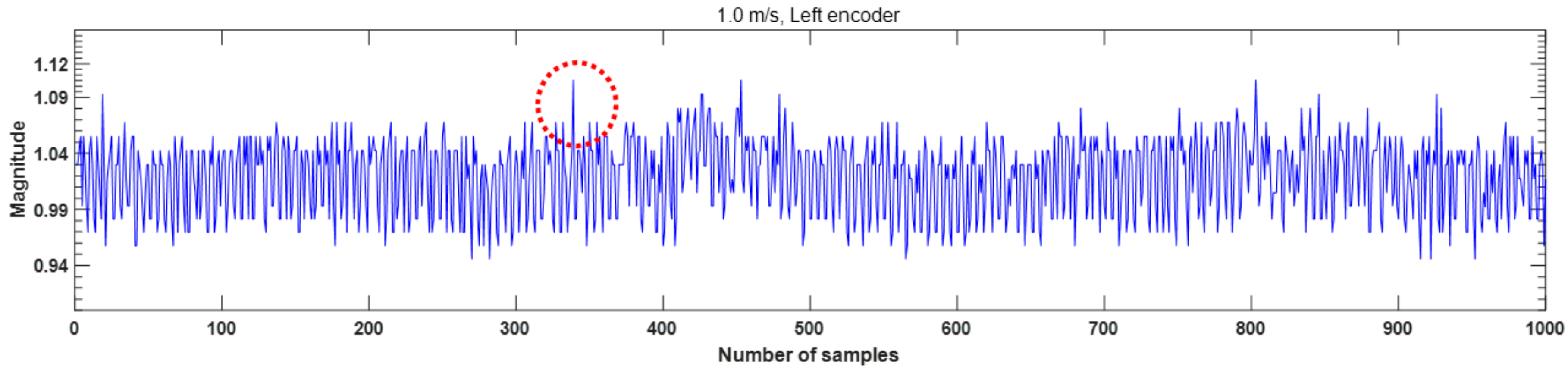
In this paper, the operation-varying threshold to be developed can be referred to as an adaptive threshold (AT) in order to distinguish it from the time-varying dynamic threshold. The adaptive threshold is critical in terms of both the adaptability to provide the robustness for automotive CPS and the sensitivity to accurately detect critical faults in the presence of anomalies. We identify a problem with respect to sensitivity and adaptability through the following simple experiment in detail. We exploit an unmanned ground vehicle (UGV) called Jackal as a target system [27]. A new adaptive cruise control (ACC) function is implemented in the target system. The operation of the physical systems can change with time while ACC driving. For the sake of simplicity, we assume that our target system performs uniform linear motion, as the Jackal UGV continues to move on a straight line with a constant velocity. During the ACC operation, states of the moving physical system might not depend on dynamics and be linear during a certain period. Figure 1 shows the real variables measured from a left encoder of the Jackal UGV. Although it drives on a straight line in a normal situation without any major fault of the sensors, we observe many anomalies for about 50 s. In other words, due to the environment uncertainty, we can see that there are frequently sensed data with noise while driving but they only show a small difference from the normal data.
In the existing model-based detection applied to the Jackal UGV, after the residual is generated using these measurements as shown in Figure 1, the difference between the magnitudes of them are examined only with the fixed threshold. The cyber system, therefore, concludes that the target system may go into the abnormal state as some faults of the encoder are detected, even though Jackal is actually in a normal state. It is no wonder that a false positive rate related to these anomalies could increase dramatically over time. This is because the fixed threshold does not respond to a changing environment where some anomalies occur naturally with uncertainty while driving. For instance, using the low fixed threshold could result in misclassifying some data of normal states into data of abnormal states, which trigger a false alarm related to the false positive error. On the contrary the high fixed threshold could lead to many false negative errors. Furthermore, for the purpose of disrupting the system, if a malicious adversary injects the malicious sensing data that enters as normal into the system through the intermediate network, the malicious data cannot be distinguished from the normal data. Consequently, the system has false negative errors.
The threshold adaptive to the dynamic environment is required to accurately detect the anomalies but should be sensitive to the changes of residuals generated. Otherwise, the false errors including FP and FN errors increases. The dynamic environment involves the environment uncertainty. The changes of residuals are mainly caused by both model uncertainties.
2.2. Challenges and Our Methodology
The state of the physical system may be gradually changed with uncertainty and nonlinearity and the cumulative impact of the undetected subtle changes during the operation might be considered negative to providing safe of CPS. In order to achieve a high level of the adaptability of the system and respond to the sensitivity of the generated residual, our first idea is to approximately identify and assess normality with residual derived from the normal operation. There are numerous methods which follow a heuristic process to support approximation derived from statistical analysis of incoming data [1,2,28,29]. The normality of the system aims to differentiate between normal and anomalous data by analyzing the tendency of the residual generation patterns. At an abstract level, identifying the normality is to define a region representing the normal condition and pick out any residual which does not belong to the normal region. Only the anomalous data that are acceptable to the system are quantitatively identified through assessing normality of the physical system during the normal driving operation. However, the data with environment uncertainty affect the quality of the tendency analysis of the residual generation pattern since they seem to be similar to the actual normal data. Another issue disturbing the normality assessment is related to model uncertainty (modeling errors) and a critical challenge is to measure quantitatively the effects of modeling uncertainty. In addition, the current normal data might not be representative of the normal state after changing the operation of the system. Hence a model representing the normality of the physical system needs to be designed with some flexibility, considering a data pattern of fluctuations caused by outlier and noise related to environment uncertainty and modeling uncertainty. Note that the normality with flexibility for data cannot be obviously defined since the uncertainty distribution is unknown. We consider a number of cases for possible normality and perform statistical tendency analysis for only one input for the same physical variable (i.e., the velocity of Jackal UGV). The normality assessment should be performed for each operation of the system.
In the tendency analysis, we assume that if noise and outlier have a small magnitude as well as being infrequent, then they are negligible. The noise and the outlier are considered the normal data even if there is big difference from normal data but it does not happen often. We, therefore, focus on an anomaly frequency of data within a given period for the data obtained during the normal operation. Although the existing statistical analysis mainly requires a large amount of data, we use only a small amount of data with a certain uncertainty limited by time intervals. Through the statistical tendency analysis, we offer a new way to allow the data itself to suggest a normality model fit for its purpose, which does not assume an underlying model. In other words, rather than trying to eliminate noise and outliers for accurate measurement, we adopt a strategy using a temporary identifier when defining the normality. Accordingly, the system is provided with an acceptable region including noisy data and outlier as well as normal data.
It is reasonable that the system requires high sensitivity with respect to low modeling uncertainty and also requires high adaptability to accommodate environment uncertainty. It is, however, difficult to achieve high levels of adaptability and sensitivity simultaneously because two competitive variables are considered to determine the AT. Besides achieving high accuracy in the fault detection, a detector should raise properly an alarm for actual faults. Its performance may be captured by two results of the FPs and the FNs. The false positive indicates that the system is actually in normal operation and any fault does not occur, and the false negative indicates that the system is faulty but the cyber system does not detect any fault. Between them, the result of the latter might be a greater threat to the safety-critical CPS rather than the former. As it is known widely, there is a trade-off relationship between them. To address these issues, our key idea is to find an equilibrium point that maximizes the other’s interests without sacrificing one’s interests and achieves low type 1 and type 2 error rates. To reach an equilibrium point between two competing variables, i.e., adaptability and sensitivity, determining an optimal threshold is formulated as an optimization problem using a nonlinear programming method at each operation. By using an equilibrium point based on normality, transient faults are differentiated by picking out the soft faults from the anomalies.
3. Adaptive Thresholds for Robust Fault Detection
In this section, we propose a transient fault detection method using adaptive thresholds, considering the sensitivity and adaptability. We carry out the statistical and information theoretic analysis during the normal operation for performance improvement in fault diagnosis using residual are characterized by quantities of uncertainty.
3.1. Overall Architecture of Fault Detection
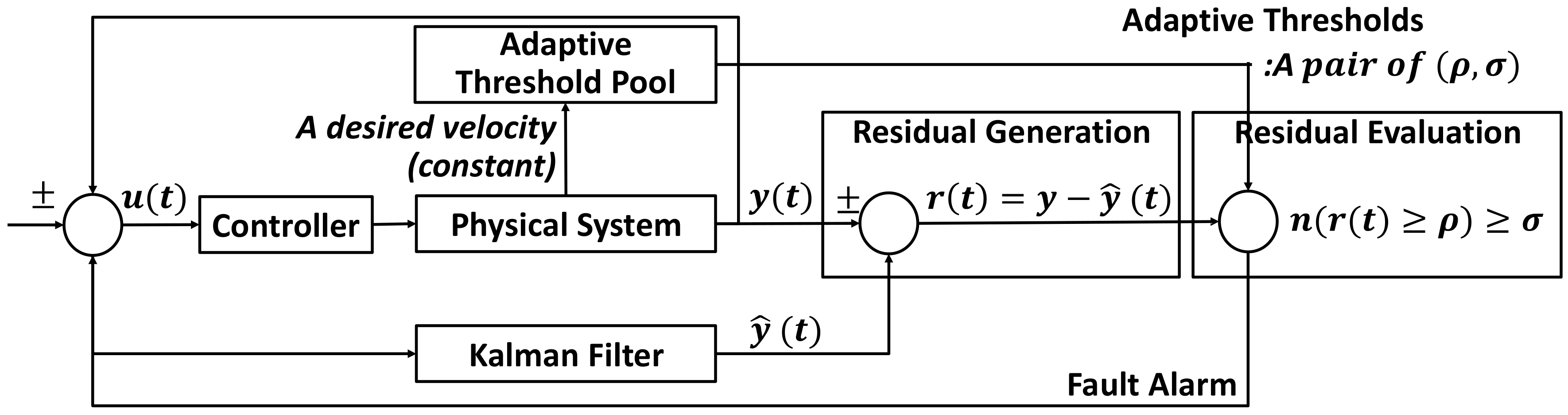
We consider a scenario of ACC with both a constant reference speed and a controlled speed which could often change depending on the safety distance behind a preceding vehicle. For ACC controlling the velocity of a vehicle, a single Kalman filter is built, tuned and then is used to perform vehicle’s longitudinal control safely. The overall architecture of the proposed fault detection using adaptive thresholds is presented in Figure 2 and consists of residual generation, residual evaluation, the Kalman filter, and an adaptive threshold pool. In Figure 2, is an estimated output, and are a measured input and a measured output at time , respectively. A residual is denoted as by subtracting the estimated value from the measured value at a given time.
In practice, the residual generation by comparing the estimated data of the Kalman filter with actual measurements and a proper threshold is chosen in the adaptive threshold pool in real time whenever the velocity of a vehicle is changed to maintain the safety distance. The adaptive threshold pool has many pairs of predefined-adaptive thresholds suitable for individual velocities at which the Jackal UGV can be driven. Each pair of adaptive thresholds consists of a reference point () and an upper boundary () as shown in Figure 2 and is determined by our method presented in Section 3.3.2.
The used Jackal UGV has many sensors including two encoders for the right and left wheels, IMU (inertial measurement unit), and GPS, and the maximum velocity is limited to 2 m/s. In our work, only two encoder sensors are used to measure the velocity as real measurements and are exploited to detect transient faults. The two wheels for each side are connected to each other using the chain. Both encoder sensors provide measurement at 20 Hz. Sensor data are gathered from Jackal by normal driving on straight lines at a constant speed. The velocities of encoders are measured in each operation distinguished by velocities.
3.2. Residiual Generation and Vehicle Dynamics Modeling
For the residual generation, dynamics of mechanical systems should be well modeled and needs to be integrated with a Kalman filter to estimate the state of the physical system. As mentioned above, the Kalman filter is already applied to some of vehicle control systems. In the Jackal UGV, the ACC application is implemented and its dynamics is integrated with the Kalman filter to estimate the velocity of the Jackal UGV. The integrated system dynamics is based on a standard differential drive vehicle model corresponding to the structure of Jackal UGV. See Appendix A for a more detailed description of the implementation.
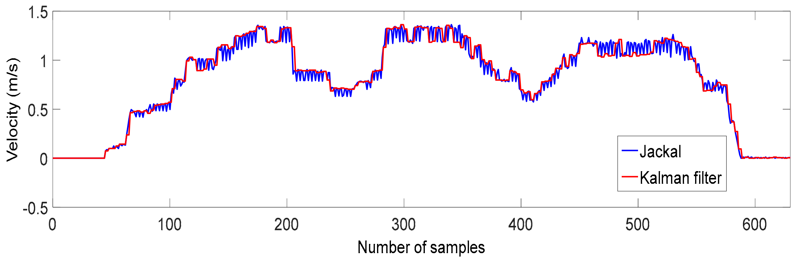
After designing the Kalman filter for Jackal, we evaluate its performance by comparing with the estimated and measured values. This experiment aims to verify that the estimation algorithm is stable and this model fits Jackal. In this experiment, during driving, the voltage as input is inserted to the Kalman filter and Jackal DC motor. The motor measures the velocity of Jackal. The Kalman filter estimates the velocity of the physical system (Jackal) based on the voltage input and the measured velocity. From Figure 3, it turns out that the Kalman filter is capable of estimating the actual velocity of Jackal, with 0.0065 of the value of root mean square errors (RMSE) in terms of precision, but we observe the small quantities of model uncertainty. Each color represents the estimated (red line) and measured values (blue line). By using both the designed Kalman filter and the encoder sensors, we can get the residuals which are generated from the estimated velocity and measured variables during a given time.
3.3. Residiual Evaluation
The goal of the methodologies presented in the subsection is to identify the normality of data in the system and to optimally determine a pair of adaptive thresholds for identifying anomalous data and transient faults. In the proposed detection system, our residual evaluation is divided into two parts: anomaly filtering and fault detection. After the first filtering identifies anomalous data for the generated residuals, the second is to detect the transient fault from the identified anomalous data. To perform each of the anomaly filtering and fault detection, the two thresholds are required. The first threshold provides a certain boundary that is able to distinguish a region with anomalous data from a region with normal data. The second dynamic threshold indicates a certain boundary that is able to distinguish transient faults from the anomalous data.
Before performing residual evaluation using two thresholds, an adaptive threshold pool needs to be preconfigured in the proposed architecture. It has one pair of two thresholds for each operation of the Jackal UGV, which is generated by using a normality model and an optimization tool. Many possibilities for the anomalous regions defined by the normality model are used to provide for optimal threshold generation. Non-linear programming is applied for one optimal pair for each operation.
3.3.1. A Normality Model
The aim of the normality model is to acquire a priori knowledge about normal data and anomalies from data obtained within a certain time under the normal operation, in order for our decision based on a priori knowledge to be applied in detecting faults for time-series data. As mentioned above, the data of the normal operation is assumed to be in the normal state and we do not have any knowledge about the magnitude or timing of the fault and anomaly occurrence. For this reason, we focus on identifying the peculiarity inherent in the normal data statistically in order to classify the data into two regions for the normal and anomalous data. To identify two regions, we apply a temporary identifier, namely a reference point, and define that the residual is in the anomalous region if the residual within the given time-window is larger than a given reference point. It means that the system can basically agree to accept the residual as normal data under the condition where the residual has the value lower than a given particular reference point within the evaluation interval. Hence, the region with the normal data is only dependent on the given reference point. In addition, to distinguish between soft and transient faults in the anomalous region, we investigate a cumulative frequency (anomaly occurrence) by histogram analysis which is a useful tool to extract a frequency pattern from the incoming residuals in the normal state. To achieve the maximum the flexibility of the normality model, it is assumed that the system agrees to tolerate many soft faults as much as possible in the anomalous regions. Such flexibility represents the maximum limit allowed for soft fault occurrences while driving on the real road. In this regard, the normality model is designed with the worst case analysis and the upper boundaries for soft faults are examined using all of the reference points.
In order to define the best-fit normal region at each velocity, we start by examining the number of occurrences of the anomalous data for all residuals. The residuals yielded from the residual generation as a function of time after driving at a certain velocity of Jackal. Given the time-series data (residuals) and the time-windows, the number of the residuals, denoted as , is counted whenever the given residual meets the reference point, . A subset of time-series data is the time window which is equal in size, and a set of the time windows is denoted as . The is any value in the region where the residual exists, and increases by the offset () gradually up to which is the maximum value in the residual region. In this paper, 0.02 is set for the offset increase of the reference point. consists of the cumulative frequency of the residual, denoted as , that goes beyond the given reference point for each time window . For all time windows at each reference point, we get cumulative frequencies which could be used to classify the anomalous region into transient and soft faults in the residual evaluation. A large cumulative frequency means that there are a large number of soft faults in the defined anomalous region. Among the anomalous regions determined by each reference point for all time windows, the worst case analysis is performed by selecting the value representing the maximum quantity of soft faults in the anomalous region. The maximum value of indicates the upper boundary at the given reference point. This process is conducted repeatedly until the reaches the maximum value () of it. At each operation , a set of upper boundaries for all reference points, denoted as , is given by:
From the set of constructed at each operation, one pair of the reference point and upper boundary is optimally determined considering adaptability and sensitivity of the system. Since the upper boundary is determined according to the reference point, the corresponding upper boundary is also optimal if the reference point is determined optimally. The optimal reference point is used for the anomaly filtering and the corresponding upper boundary is used for the fault detection.
3.3.2. An Equilibrium Point
In order to improve performance, the system requires high sensitivity with respect to low modeling uncertainty and also requires high adaptability to accommodate environment uncertainty. In fact, these non-functional requirements are difficult to satisfy simultaneously because there is a trade-off relation between them. In this normality model, the size of the normal region defined not only highly depends on the levels of sensitivity and adaptability for the generated residual, but each level of the sensitivity and adaptability is also associated with the false positive rate and the false negative rate, respectively. In our normality model, an increase in the reference point leads to an increase of the region covering the data likely to be in the normal states. However, the probability that the data may actually be anomalous data increases. It means that while the system provides higher adaptability and flexibility, it cannot guarantee high detectability due to an increase in the false negative error rate when the high reference point is used. In contrast, when the system meets high sensitivity as the reference point decreases, it brings about an increase in the anomalous region. Hence, while it is capable of recognizing the anomalous state well and increasing the degree of precision related to modeling uncertainty, it would be a major cause of occurrences of false positive errors.
In terms of adaptability, a higher reference point is preferred while a lower reference point is preferred in terms of sensitivity. We determine one reference point as an optimal solution which can represent the best possible compromise between two competing objectives. In other words, a reference point can be represented as a single point, namely an equilibrium point, derived from the trade-off relationship of these objectives. When we find out an equilibrium point that meets the specified conditions where the performance of the sensitivity is maximized without sacrificing the performance of the adaptability, it can be a reasonable and fair solution. After two performance measures are defined to represent the performance of the two objectives, an equilibrium point is formulated as nonlinear programming which can solve optimally. Based on the normality model, two performance measures are calculated by using the defined regions for the anomalous data and transient faults which are derived from each of the combinations of both the reference point and the upper boundary.
First, the concept of information uncertainty is adopted to represent the level of sensitivity. The uncertainty denoted as , of the system means that how uncertain the system is about the presence of the transient faults, not soft faults, in the anomalous region defined by our normality model. It also represents the influence of the false positive error rates with respect to the anomalous region. Therefore, the uncertainty of the system at each reference point for all velocities is given by the conditional entropy which quantifies the amount of information describing the event that transient faults might exist in the suggested anomalous region. When the discrete random variable X and Y taking a certain value and , respectively, let represent whether the given residual is close to the normal or anomalous state so that = 1 means that the residual is anomalous, and = 0 means that the residual is normal. Let represent whether the residual where belongs to is a transient fault or a soft fault. = 1 indicates that the residual is a transient fault, and, otherwise, the residual is a soft fault. According to information theory, the conditional entropy of Y given X is defined as Equation (2) from which we can obtain the conditional entropy at each reference point for all velocities, which is normalized from 0 to 1.
Second, the detectability is defined to represent the adaptability. The detectability, denoted as , of the system means that how much the detection performance depends on the size of the normal region defined by the normality model. As mentioned above, higher adaptability results in the large size of the normal region so that it induces an increase in the false negative error rate. The level of the detectability is defined as a weighted harmonic mean of recall and precision, called -score. Precision provides the information on how accurately our model predicts the given residual as an actual fault. Recall provides the information on how accurately our model captures faults which should be an actual fault. To have a balance between the two, -score is commonly used as a measure of an accuracy in binary classification. In our work, we give the recall more weight than precision because, in safety-critical applications, the false negative errors are worse and more dangerous than false positive errors in general. -score bounds from 0 to 1 from Equation (3).
For the sake of the simplicity in calculation, we exploit the number of offsets to calculate the reference point rather than using the value of the reference point directly. Note that the number of offsets starts from one and the maximum number of offsets is different for each velocity of Jackal UGV. Given the data set of the uncertainty of units, the uncertainty function is with the negative slope by using the uncertainty level as a function of the number of offsets. Hence we define the function of the uncertainty representing the sensitivity as the following form:
where is the number of offsets corresponding to reference point as the explanatory variable, and the constant variables and , are given by using linear regression analysis. We also use a linear regression analysis to find the relationship between detectability and the number of the offsets. Given the data set of the detectability of units, since the number of offsets to the reference point has a positive relationship to the detectability levels representing the adaptability, the relationship is defined as follows:
where the constant variables and , are also given by using linear regression analysis. Our approach is to determine the point is that as the reference point increases, the sum of the expected amount of the adaptability and the expected amount of the sensitivity that is obtained is maximized. By nonlinear programming, a two-variable constrained optimization problem can then be written as:
where is to perform transformation of the function through composition transformation to reflect the effect of the maximum number of offsets depending on the velocity, and described by
This transformation does not change the solution of the original problem and consists of the reflection about Y-axis and translation with the offset vector (, 0), where is the maximum value of X-axis. The method of the Lagrange multiplier that is applied to find a point at which the function S(x) values are maximized:
where is the Lagrange multiplier. The variable to be optimal (a global max) which fully meets the necessary condition for the Lagrange function is obtained as Equation (9).
Note that a conversion to reference point is required since the determined indicates the number of offsets. As this equilibrium point ( corresponding to one reference point is determined, one pair of the reference point and upper boundary is finally determined from the set of and is stored in the adaptive threshold pool for fault detection.
4. Performance Evaluation
In this section, we evaluate the performance of the proposed fault detection method using the adaptive threshold, denoted as AT, based on the model-based method by comparing it with two dynamic thresholds. One of the dynamic threshold methods is based on root mean square (RMS) which is commonly used to generate a dynamic threshold and is denoted as RT [30,31,32]. We use RMSs for each time-window . The other of the dynamic threshold methods is to find a knee point between the error bound and the number of fault occurrences and is denoted as KT [1,2,28,29].
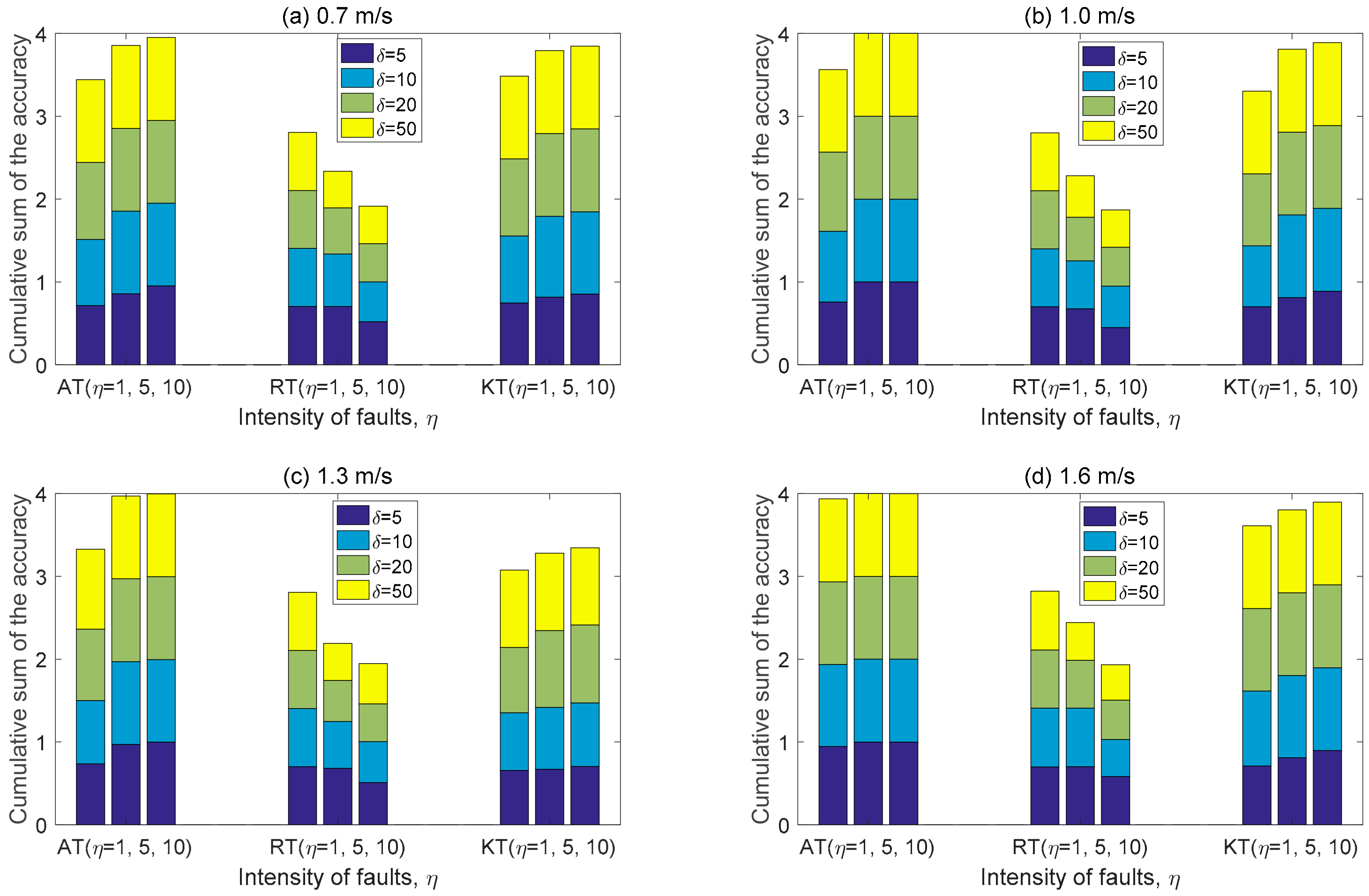
We use both the training and test data as residuals which are obtained from the encoder sensors while Jackal UGV drives on the real road at each of several velocities from 0.7 m/s to 1.6 m/s by 0.3 m/s. Training data are used to generate AT for the adaptive pool as well as RT and KT. Test data are used for performance evaluation. Table 1 lists all of the thresholds generated according to AT, RT, and KT for each velocity. However, the values of RT are not described in detail and is only mean values for each velocity because they are different for each time-window . In the residual evaluation, we use the of the first threshold for differentiating the anomalous data from the normal data before the is used as the second threshold to detect transient faults from the anomalous data. Note that the difference between the first thresholds () of AT and KT is the largest at the velocity of 1.3 m/s.
To demonstrate the high accuracy and the low type 1 and 2 errors with the change of the operation, we present the recall, accuracy, and precision as assessment outcomes when divergent scenarios are adopted. The high recall represents the low false negative error rate, which is calculated by . The low false positive rate results in the high precision which is calculated by . In our experiments, four scenarios associated with the velocity changes, and three scenarios with respect to a type of transient fault are designed. Furthermore, for each experiment, the variables for the duration and intensity of faults injected are varied. The duration and the intensity are useful to assess adaptability and sensitivity, respectively.
We inject constant, random, noise faults for performance evaluation. It is worth attempting constant faults because they show how well the adaptive thresholds basically work in accordance with the controlled environmental parameters such as the intensity and the duration of faults. The random fault detection is very meaningful in terms of how sensitive it is to identify faults similar to the original data because one value is selected from the distribution of the values of the original data and is used as a fault. Finally, the noise fault is injected with the magnitude similar to the noise which is most common and can occur in nature. It is worthwhile noting that the adaptive threshold generation is sufficient for statistical analysis of the data obtained in the normal operation.
For each experiment, the timing of fault occurrence is selected randomly and the number of fault occurrence is three, the magnitude (intensity) of the fault is always different according to types of faults. While three types of faults are injected into real measurements, the duration of faults are varied from five samples (250 ms) to 50 samples (2.5 s). The evaluation is conducted repeatedly for 50 at the given time window (i.e., = 100).
4.1. Constant Faults
Constant faults are just to add the constant magnitude to the original values. Rather than injecting several constant values selected randomly, the constant magnitudes are generated by using the predefined values for intensity in order to give consistency to the constant values. The constant magnitude is determined by using the predefined intensity and the magnitude of several samples picked randomly from the original data. Hence, the magnitude of the constant fault is the magnitude of the picked sample multiplied by the intensity plus the magnitude of the picked sample. The values of the intensity used is = {1.5, 2, 5} [33]. The magnitude for constant faults, denoted as , is calculated by
where the magnitude of the data that is randomly selected is denoted as , and is one of the values of the intensity. From Equation (10), when = 1.5 is applied, the constant faults with one value in the range of ] are generated by about 100% of the total constant faults where is the mean value of the training data at the certain velocity. When = 5 is applied, constant faults in the range of ] account for about 100%.
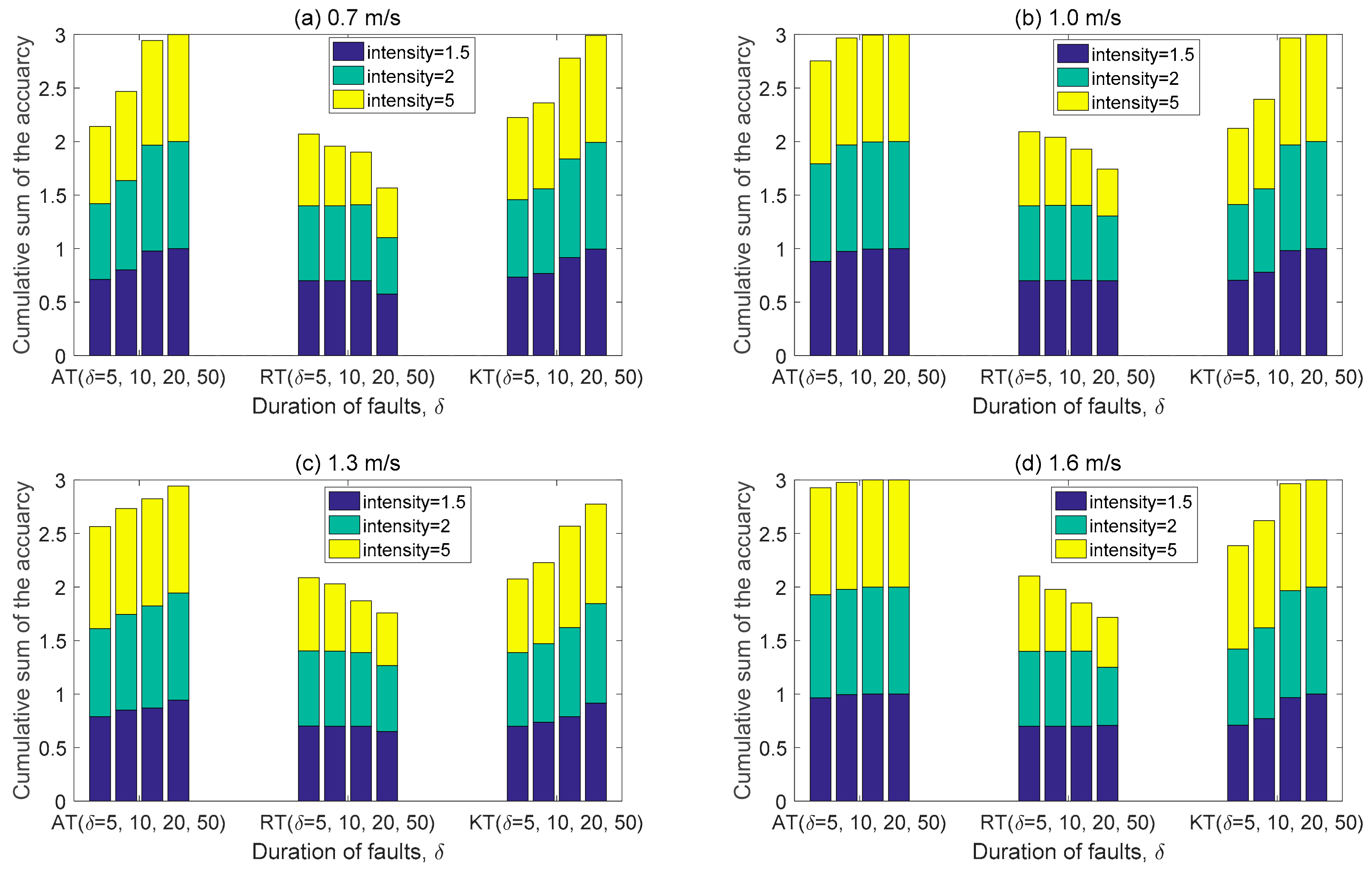
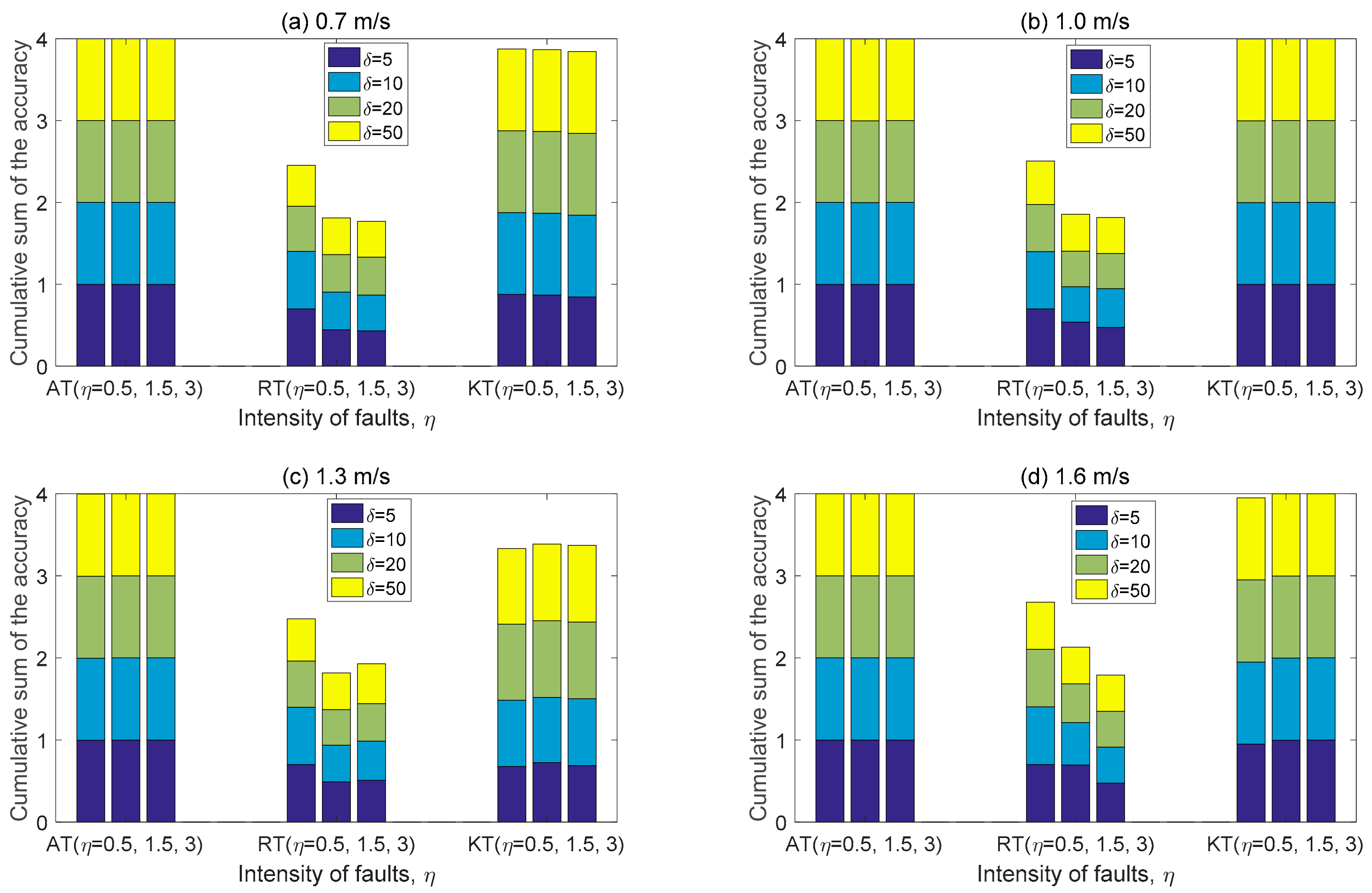
Figure 4 shows the performance results in terms of accuracy calculated by . A true positive (TP) means a transient fault that is correctly identified, a true negative (TN) is a normal data including a soft fault that is correctly identified, an FP is an actual normal data that is identified as a transient fault, and an FN means an actual faulty data that is identified as a normal data in fault detection.
Overall, AT demonstrates better performance than RT and KT. For all velocities, it shows the trend that the performance of AT is not significantly affected by the magnitude of the intensity unlike KT and RT, and AT has also high performance level regardless of the duration as the velocity increases. Only when the duration is low ( 5) at the low velocity (0.7 m/s), the performance of AT is less than 2% (three samples) of that of KT. Under the small duration of the constant faults injected at low velocity, the acquired measurements are very small and the change (standard deviation) in the acquired measurements is not large. In this regard, the small difference between the given thresholds of (i.e., 0.117679 of AT and 0.11 of KT) seems to have a great effect on the determination of the anomalous region. Except in the case above, the performance of AT overcomes those of RT and KT performance regardless of the duration and intensity as the speed increases. Thus, our AT shows good detection results because it is sensitive to the very small intensity of injected faults.
In the case of KT, although the accuracy performance of KT shows the similar tendency to that of our AT, it notes that the accuracy of KT is highly affected by the length of duration rather than the magnitude of the intensity. For example, the performance at the small intensity ( is about 4% lower than that at the largest intensity ( = 5) at the lowest speed. In addition, at the short duration ( the performance of KT is not any the better even if the velocity increases. This result seems to be due to the high value of the second threshold which may cause an increase in FN.
Regardless of velocities, as the duration and intensity are shorter ( and smaller ( = 1.5 and 2) respectively, the RT has better performance. From these results, we find out that RT is sensitive to small changes. However, if the intensity is higher, both the TPs and FPs increase at the same time while the TNs decreases. This fact is again evident from plotting the precision.
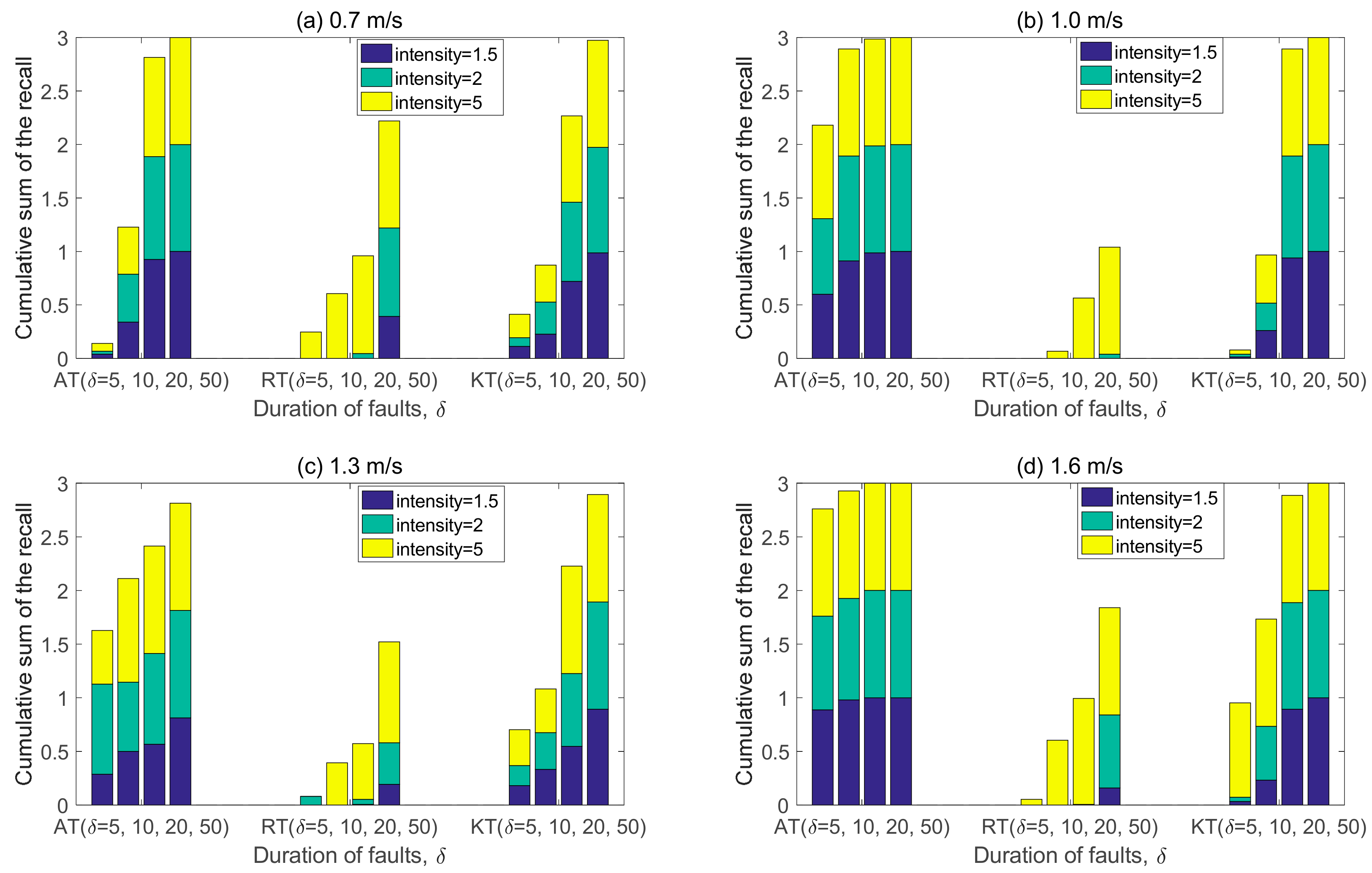
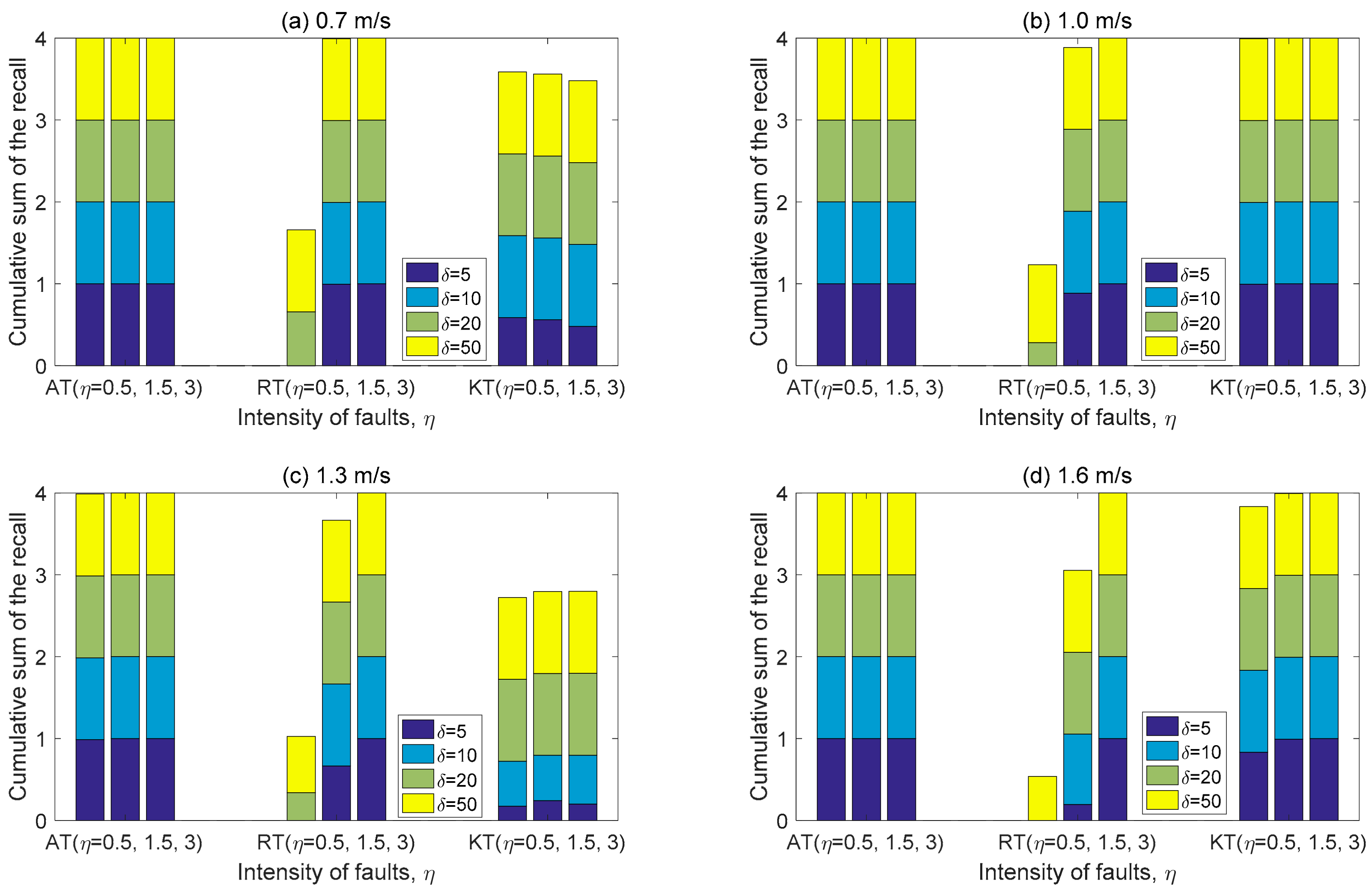
Figure 5 shows the recall presenting the relationship between TPs and FNs. As mentioned above, because our adaptive thresholds are designed for the safety-critical application, achieving the low false negatives is very important. Since the magnitude of the constant faults injected is not large, FNs tends to increase in all thresholds as the duration decreases.
In other words, such data are actually the faults although they are identified in the normal state.
Especially, RT has a significantly higher FNs and fewer TPs when the duration and the intensity are shorter and smaller, respectively, resulting in no recall or very low recall. In the case of KT, since FNs is much higher in short fault duration ( than in large duration even though the velocity increases, its recall performance is poor. This is because the shorter duration never helps determine the anomalous region by the first threshold of KT.
In AT, as the duration increases, the data to be faults within the particular anomalous region increases in the number and the detection is performed well by the second low threshold, which is more sophisticated than that of KT. As the velocity increases, the AT performance becomes more distinct because the proposed optimal thresholds are adapted well to the high uncertainty in the driving environment where the data variation is high. Only at the recall at 0.7 m/s and , the recall appears low since the FNs of AT is a little larger than those of KT. This seems to be due to the wide normal region because the first threshold of AT is slightly larger than that of KT when its velocity is the slowest.
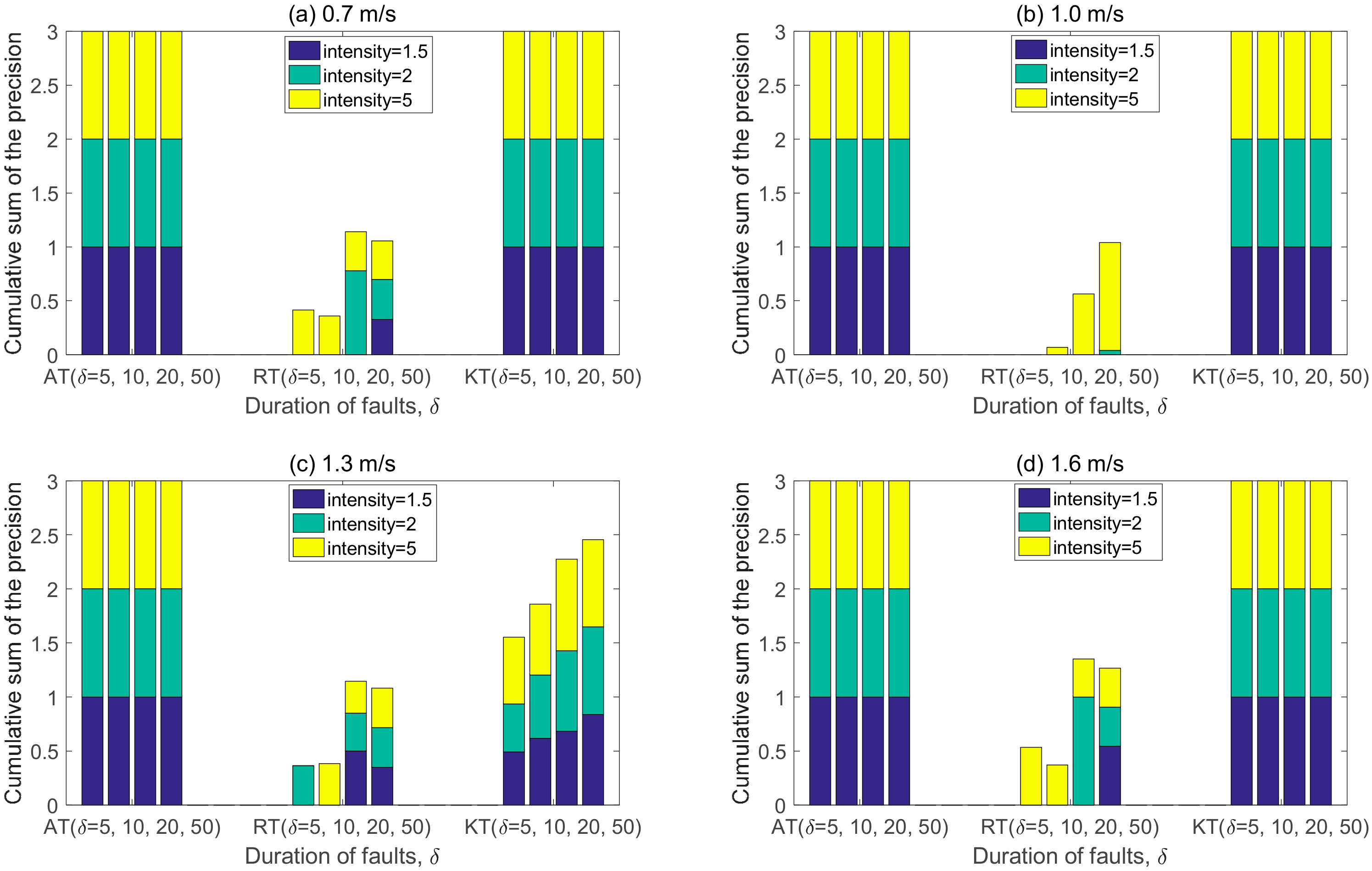
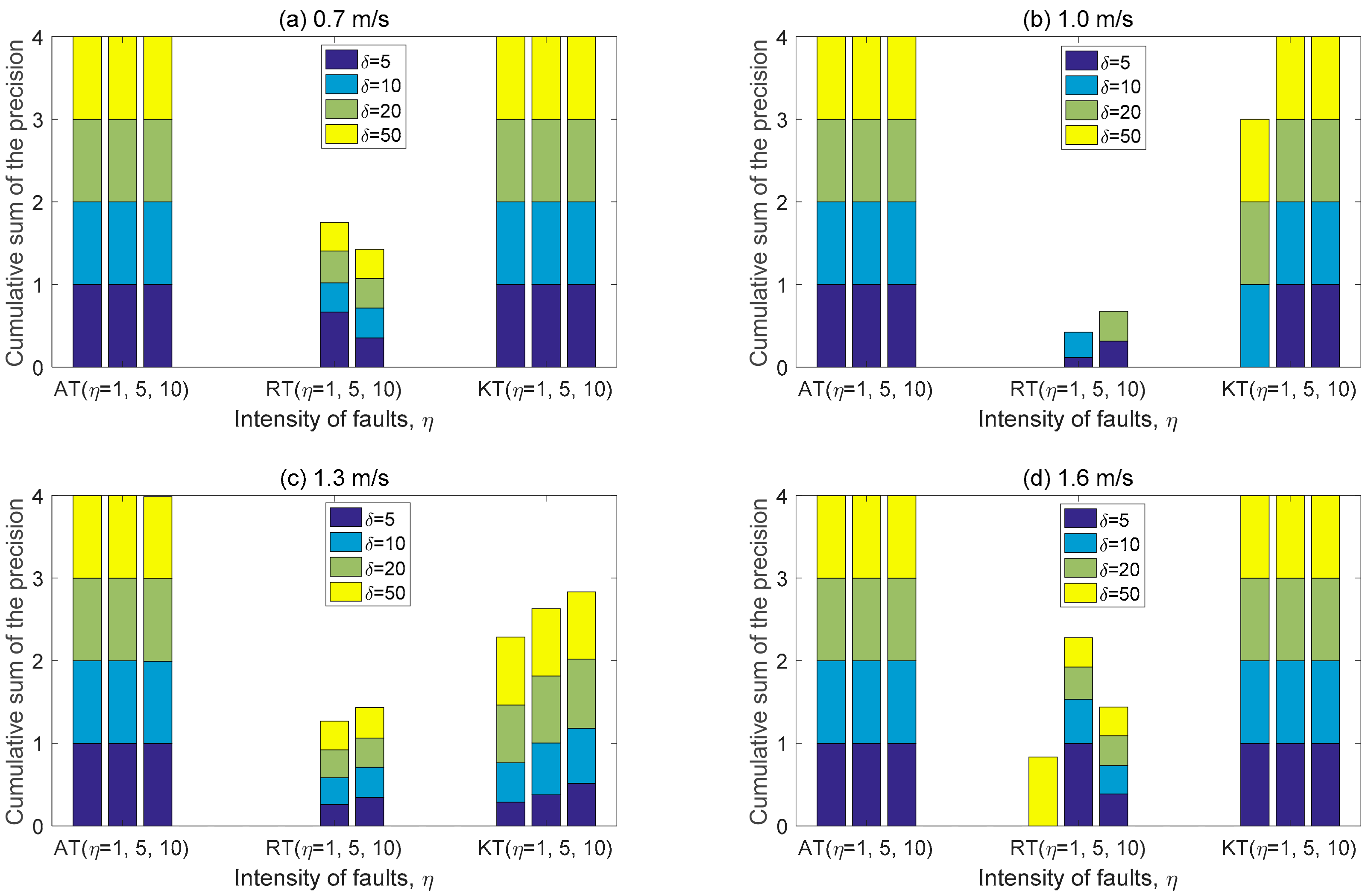
The precision with regard to false positives is shown in Figure 6. Both AT and KT which show 0% of the FP rate for all velocities conduct the elaborate detection of faults from the anomalous region. As mentioned earlier, in the case of RT, both FPs and TPs are increased at the same time as the intensity is larger and the duration is longer. On the contrary to this, RT does not respond to the small changes to which the intensity and duration are applied with the low values.
4.2. Random Faults
The magnitude of random faults injected in our experiments is determined by using one value selected randomly in the distribution of the magnitude of the original data at each velocity. The duration variation follows that of the constant fault. The intensity is by which the selected magnitude is multiplied. The magnitude of random faults is given by
where is a random number drawn from the standard normal distribution, is one of the intensity values, and and are the mean value and the standard deviation of the training data at the certain velocity respectively.
The accuracy of the random fault detection is presented in Figure 7. At all velocities except for 0.7 m/s of the velocity, AT achieves the best performance close to 100% when exceeding the intensity of a certain magnitude (. As with constant faults, AT has lower performance than KT only in the shortest duration and velocity ( and it seems to be due to the slightly high threshold of AT at the lowest velocity. From Equation (11), when = 1 is applied, the random faults with one value in the range of ] are generated by about 47% of the total random faults and random faults in the range of ] account for about 82%. Hence, when = 1 is applied, these results are so meaningful in terms of sensitivity to small changes. The ability to identify them is superior at all velocities compared to other methods when the faults with the magnitude similar to that of the original data are injected. Obviously, the larger the intensity is, the closer to 100% the performance of AT is.
Unlike AT, the accuracy of KT is significantly influenced by the intensity and duration irrespective of the velocity. Furthermore, when = 5 and 10, although the magnitude that goes beyond the value of account for about 47% and about 71% of the total faults generated, respectively, the performance of KT is not as good as that of AT. RT tends to decrease in the performance as the duration and intensity increase. In the case of RT, when the intensity is small ( = 1), the TPs do not increase regardless of the duration, but the actual normal data are identified well. When the intensity is medium and high, the TPs increase but the ability is insufficient for identifying the actual normal data as the duration increases. Therefore, these results mean that KT and RT are not adaptive and sensitive even though they are determined dynamically.
Figure 8 shows the results of the recall of three methods. It is similar to the tendency of the accuracy of both AT and KT except RT. When the velocity is 0.7 m/s, the recall performance is low as the duration becomes shorter. This is due to the increase in the occurrence of FNs, that is, the faults are mistaken as normal data. The cause of the FN increase seems to be closely related to the size of the time window. However, from the results, we find that this tendency shows that AT adapts quickly as the intensity becomes stronger. At the velocity above 1.0 m/s, we also find that AT and KT produce many FNs only when = 1. However, the frequency of FNs in AT is much smaller than that of KT even though the duration is very short.
Furthermore, as the intensity and the velocity increase, AT does not generate any FN error, but KT still has many FN errors. In the random faults, RT is unable to detect faults with similar size to the original data, and classify almost all injected faults as normal data. However, the intensity and duration become larger, the amount of mistaken data become less. In the case of RT, when the intensity is small ( = 1), the FNs increases regardless of the duration but no faults are detected. When the intensity is medium, the FNs decreases as the duration increases. The FN frequency is very low when the intensity is high and the duration is small. Only when the intensity is large enough to identify the difference, the RT is applied to detect faults.
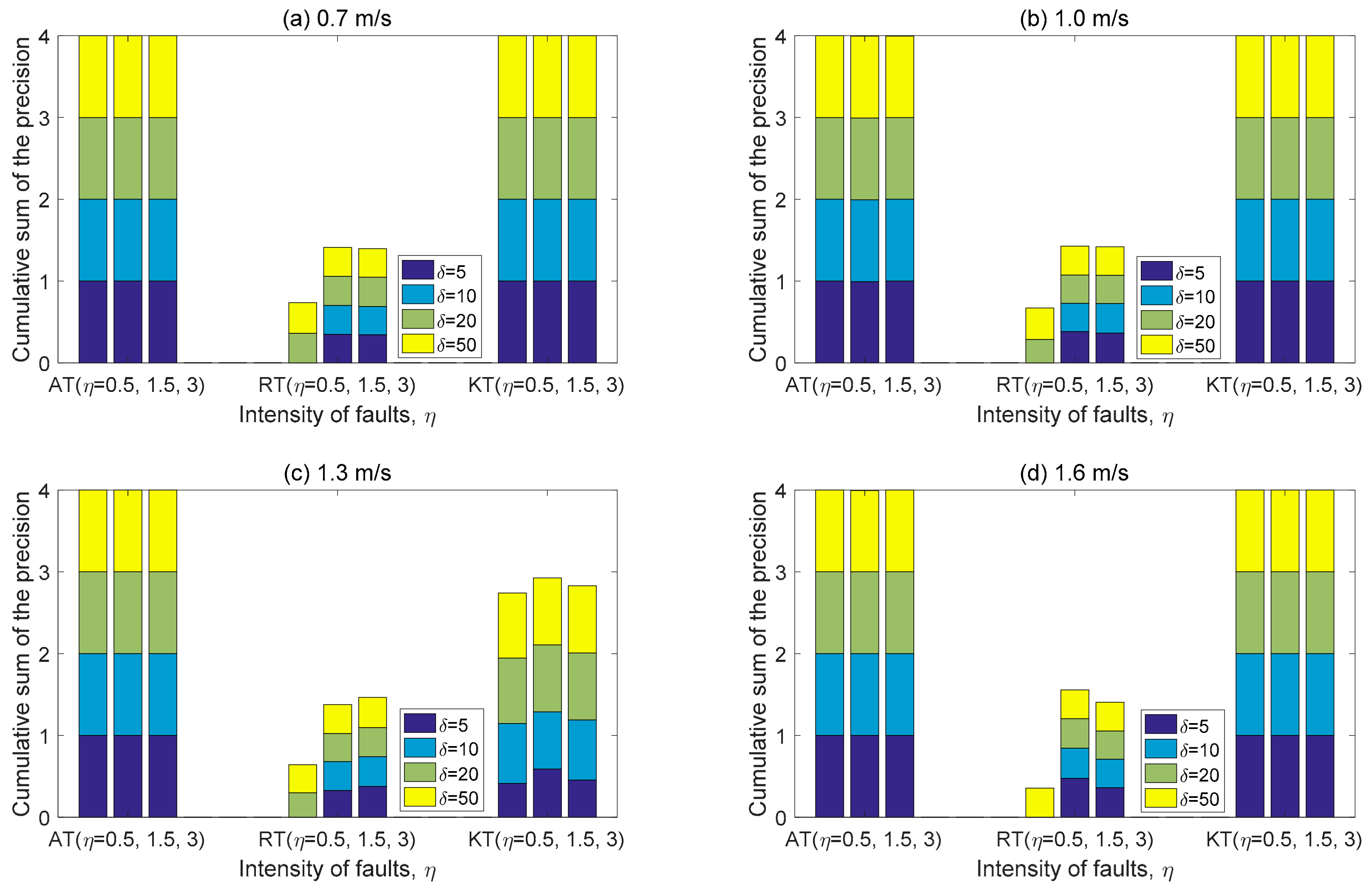
The precision results of each method are shown in Figure 9 according to the magnitude of intensity. At all velocities, AT shows the best performance and 0% of FP occurrence. At 1.0 m/s and 1.3 m/s, there is a significant difference in performance between AT and KT. The difference between the two thresholds at all intensities seems to make an appreciable difference to the performance. As mentioned above, the difference between the first thresholds () of AT and KT is the largest at the velocity of 1.3 m/s. Since the small threshold of KT, compared to that of AT, results in the wide anomalous region, in random faults, KT shows low performance with many FPs that occur constantly for all conditions. In contrast, AT does not have any FP at all. At 1.0 m/s, since the second threshold ( of KT is too high, KT fails to detect the random faults under the lowest intensity ( = 1) and the shortest duration (. In the case of RT, the performance is better as its velocity increases but the precision is very low. The intensity and the duration are higher simultaneously, a large number of FPs also occurs while TPs are increased. Especially, when the injected faults are similar to the magnitude of the original data (), the detection performance is zero since almost all injected faults are classified as normal data. This is because all, including the normal and anomalous, data are identified as the normal data when .
4.3. Noise Faults
In our experiment, injecting noise faults aims to assess the detectability under Additive Gaussian white noise (AGWN) that is most common in communication systems and can occur in nature. This fault is generated by adding the one value drawn from in a zero-mean normal distribution with a given variance to the magnitude of the original data at each velocity. The performance can be bound to vary on the given variance, but for the purpose of noise faults involved in these experiments, the variance is fixed at one. The duration variation is the same as that of the constant and random faults. The magnitude of noise faults is determined by:
where is a random number drawn from the standard normal distribution, and is one of the intensity of . This intensity used is quite different from those of the random faults and was already used in the research of SHARMA et al. [25]. From Equation (12), when = 0.5 is applied, the noise faults with one value in the range of ] are generated by about 0% of the total noise faults where is the mean value of the training data at the certain velocity, and them in the range of ] account for about 100%. Note that the magnitude of noise faults is much larger than that of random faults.
Figure 10 shows the detection accuracy of the three thresholds for noise faults. For all velocities, AT has the precision of 100% and is not affected by the duration and intensity. KT shows that its performance is mainly low at the shortest duration and the lowest intensity for all velocity when it is compared to other conditions. From these results, we discovery that KT is less sensitive to the trivial noise. Although KT has the worst performance at 1.3 m/s for the noise faults, the performance of the noise faults is increased slightly more than that of random faults. In the case of RT, the accuracy is better when the intensity is smaller and the duration is shorter. However, it can be predicted that many FPs can occur since it responds sensitively to small changes. This remark can be seen in the graph of precision.
In Figure 11, we present the results of recall at each velocity. We can see that in AT, no FN has occurred for all velocities. In the case of KT of 0.7 m/s, the FNs occur unconditionally when the duration is 5 for all of the intensities. Even as the velocity increases, the sensitivity to small changes is still low when the duration is short. It indicates that KT is not capable of responding to the very short occurrence of noise. In KT, the levels of intensity have little effect on the noise fault detection since the magnitude of the noise faults is already too large as mention above. As with other faults, the recall of KT is the worst at 1.3 m/s, and FNs increases at both regardless of the intensity, since the lower first and the high second thresholds influences are still on it.
In case of RT, the recall is better than that of KT at 0.7 m/s and is comparable to that of KT except for 0.7 m/s when the intensity is high (). From this graph, we can find that RT has the ability to detect faults better than KT in the case of noise with a magnitude of a certain level (.
Figure 12 depicts the results of precision. From these results, it can be seen that AT is well adapted to the large changes from the small changes by using the proposed thresholds for all velocities, and any FP has not occurred at all.
In the noise faults, except for 1.3 m/s, as KT does not have FPs, its precision achieves 100%. However, at 1.3 m/s constant FPs occur regardless of the intensity and the duration, but TPs increase as the duration becomes higher. In addition, KT at 1.3 m/s shows better precision than KT in random faults. This is because the magnitude of the noise faults is large enough to be detected even though the intensity for them is the lowest (. Nevertheless, the FPR (false positive rate) of the KT is in the range of about 58% to about 18% at 1.3 m/s. In RT, the FP is increased significantly as the duration increases at the certain levels of intensity (. When the intensity is below 1.5, RT is not capable of detecting noise faults.
4.4. Discussion
The FNR (false negative rate) and FPR of the experimental results for all scenarios are averaged and shown in Table 2. Note that the magnitude of injected faults is the smallest in constant faults and the largest in noise faults. Random faults are distributed in all ranges of the magnitude according to the intensity. For all types of faults regarding all of the intensity and duration AT does not generate any FP for all velocities, but KT does show an average 27% of FPR only at 1.3 m/s. RT shows about 64% FPR for all faults regardless of velocity.
AT shows 0% FNR for all velocities in noise faults but it has mean 7% FNR for random faults, and mean 12% FNR for constant faults, respectively, except for 0.7 m/s. KT show about 10%, 29.5%, and 38% FNR for noise, random and constant faults, respectively, except 0.7 m/s. RT not only has about 52.3% and 78.5% FNR, respectively, except 0.7 m/s for random and constant faults, but also, about 27% FNR is shown for noise faults. The reason for the poor FNR performance for constant fault injection for all thresholds seems to be that the designed intensity is too small to be distinguished from normal data and transient faults.
From the above results, we demonstrate that the AT has enough sensitivity to small changes and adaptable to various changes and has the dependability enough to support the safety for CPS. However, the performance of the AT is degraded only at both the lowest velocity and the shortest duration, probably because the variation and the values of the original training data are too small to identify the differences in the large time-window size at the lowest velocity. There is a need for further investigation related to the size of time window as the velocity slows down, which needs to be made smaller than = 100.
5. Conclusions
The critical faults have high potential to threaten the safety of automotive CPS. In particular, the transient faults in the anomalous data causes the unexpected behavior of the system during operation; however, their effects might not appear immediately. In this paper, in order to drive CPS into the stable state and to perform the operations of automotive CPS safely by detecting transient faults, we have developed a novel way to determine the adaptive threshold as the equilibrium point between competing variables. In the experimental evaluation using the real UGV data, our threshold yields a significantly better accuracy, recall, and precision than RT and KT. Against noise faults, AT shows nearly 100% accuracy, recall, and precision at each of the operation, regardless of the intensity and duration of faults. Under the constant faults, it achieves the accuracy from 85.4% to 100%, the recall of 100% from the lowest 54.2%, and the precision of 100%. AT also gives the accuracy of 100% from the lowest 83.2%, the recall of 100% from the lowest 43.8%, and the precision of 100% against random faults. In this regard, we have demonstrated that the proposed generation method enables adaptive thresholds to enhance the adaptability and sensitivity to the various environments and modeling errors and achieves a high level of detectability simultaneously in fault detection.
Since our method is based on the model-based detection that performs both residual generation and evaluation, the dynamics of the targeted physical system as one of automotive CPS is first modeled and is integrated into the Kalman filter to estimate the state of the physical system and generate the residual. Furthermore, we design a structure that adds the adaptive threshold pool to the basic structure of the model-based detection and extracts the pair of thresholds from it according to the referenced velocity. In order to cope with fluctuations caused by noise, environment uncertainty, and modeling uncertainty, the normality of the physical system needs to be considered with some flexibility and it also needs to find out optimally how to determine an adaptive threshold which plays an important role in distinguishing faults from anomalous data. In our approach, since the normality cannot be obviously defined due to lack of prior knowledge of the fault occurrence, we should consider many different possibilities of normality by examining the residual under normal driving conditions. By statistical analysis, the normality is assessed in order to define the normal and anomalous states from the data obtained under the normal operation of automotive CPS. The specified normality model allows us to get various pairs of thresholds that can be used to detect transient faults in the residual evaluation. We find out one optimal pair achieving the best performance required by CPS as the adaptability and sensitivity are considered to minimize uncertainties of modeling and environment. To do this, after the performance measures that can represent two comparable variables are defined, the optimization problem is formulated by using the nonlinear programming method in order to maximize the interests of two measures.
These experimental results show that there is an obvious difference among the performance results of three thresholds. In terms of accuracy, recall, and precision, performance evaluation of our AT is performed based on various scenarios, compared with the performance of other dynamic threshold techniques. When the performance is analyzed by varying the duration and intensity for three kinds of faults, AT generated by the proposed method is not influenced by the change of the intensity and duration at each velocity. KT could not detect faults properly if the intensity is low or/and the duration is short. Since RT is sensitive to small changes of measurements, its performance is significantly changed according to duration and intensity and showed similar performance regardless of velocity.
The AT method helps prevent misleading interpretations that the cyber system concludes some intermittent anomalous data and noises as fatal faults even though they occur naturally, disappear soon, and do not affect adversely the control of the system. AT is not only competent to diagnosis the faults with high levels of sensitivity and adaptability, but also it achieves good performance with only a small amount of data with a certain uncertainty limited by time intervals. In particular, it is noteworthy that the thresholds are optimally determined in response to the obtained measurements that change significantly as the velocity is varied because it proves that the intensity and duration have nothing with the performance of AT. Therefore, the adaptive threshold generated from the combination of our threshold generation method and the normality model can be a good criterion for distinguishing between normal and anomalous states as well as detecting faults. The AT determined from the equilibrium can be said to have high degrees of adaptability and sensitivity. In future work, at lower velocities, the performance of AT needs to be improved by varying the time window size.
Author Contributions
Conceptualization, Y.B.; Methodology, Y.B.; Resources, M.J.; Supervision, Y.B.; Writing—original draft, Y.B.; Writing—review and editing, Y.B.
Funding
This research was supported in part by Global Research Laboratory Program (Grant No.: 2013K1A1A2A02078326) through the NRF of Korea.
Acknowledgments
I would like to thank researchers (in Convergence Research Center for Future Automotive Technology, DGIST), Daehyun Kim and Soohyeon Kwon, for providing technical support for the modeling of dynamics of mechanical systems.
Conflicts of Interest
The authors declare no conflict of interest.
Appendix A
For the residual generation, dynamics of mechanical systems is modeled as follows. Let the dynamics be given by the following standard state equation in a vector form:
where A is a 2 × 2 square matrix of the constant coefficients, and B is a 2 × 1 matrix of the coefficients to weight inputs because both matrices A and B are determined by the structure and elements of Jackal. The coefficients for both matrices A and B is described in motor modeling as mentioned below. The set of two state variables is represented as a state vector of which each state variable is a time-varying component, an input vector consists of inputs at time . Since many physical systems have the null matrix to the input vector u, the output equation is given by:
where is a vector of the output variables, and C is a 1 × 2 matrix of the constant coefficients to weight the state variables. The system matrices A, B, and C can be expressed with the gear ratio of 25:1 (N = 25) in Equations (A1) and (A2), respectively. The state vector is presented in Equation (A3) as a column vector of length 2.
where and represent the armature motor current and the wheel speed, respectively. The motor used for Jackal is modeled by using the standard equation for a brushed DC motor.
In the Equation (A4), is defined as the armature voltage and is the armature resistance. , , and represent the back-EMF (electromotive force) voltage constant, the motor rotational speed and the armature inductance, respectively. The motor torque and the load torque can be represented as
where is the motor torque constant, and indicate the moment of inertia of the motor and vehicle, respectively. and represent the viscous friction coefficient of the motor and vehicle, respectively. The values used in coefficients of the Kalman filter for Jackal are summarized in Table A1.

Table A1.
Parameters used for the Kalman filter.
| Parameter | Value | Parameter | Value |
|---|---|---|---|
| 24 | 4.49 × 10⁻² | ||
| 0.5 | 4.45 × 10⁻² | ||
| 2.2 × 10⁻⁴ | 5.5 × 10⁻⁴ | ||
| 0.05 | 25 |
References
- Satopaa, V.; Albrecht, J.; Irwin, D.; Raghavan, B. Finding a kneedle in a haystack: Detecting knee points in system behavior. In Proceedings of the 31st International Conference on Distributed Computing Systems Workshops (ICDCSW), Minneapolis, MN, USA, 25 July 2011. [Google Scholar]
- Park, J.; Ivanov, R.; Weimer, J.; Pajic, M.; Lee, I. Sensor attack detection in the presence of transient faults. In Proceedings of the 2015 ACM/IEEE International Conference on Cyber Physical Systems (ICCPS), Seattle, WA, USA, 14–16 April 2015; pp. 1–10. [Google Scholar]
- Moseler, O.; Isermann, R. Application of model-based fault detection to a brushless dc motor. IEEE Trans. Ind. Electron. 2000, 47, 1015–1020. [Google Scholar] [CrossRef]
- Huang, S.N.; Tan, K.K.; Wong, Y.S.; De Silva, C.W.; Goh, H.L.; Tan, W.W. Tool wear detection and fault diagnosis based on cutting force monitoring. Int. J. Mach. Tools Manuf. 2007, 3, 444–451. [Google Scholar] [CrossRef]
- Khalid, H.M.; Khoukhi, A.; Al-Sunni, F.M. Fault detection and classification using Kalman filter and genetic neuro-fuzzy systems. In Proceedings of the Annual Meeting of the North American Fuzzy Information Processing Society, El Paso, TX, USA, 18–20 March 2011; pp. 18–20. [Google Scholar]
- Gao, Z.; Cecati, C.; Ding, S.X. A survey of fault diagnosis and fault-tolerant techniques—Part I: Fault diagnosis with model-based and signal-based approaches. IEEE Trans. Ind. Electron. 2015, 62, 3757–3767. [Google Scholar] [CrossRef]
- Amin, S.; Litrico, X.; Sastry, S.S.; Bayen, A.M. Cyber security of water SCADA systems—Part II: Attack detection using enhanced hydrodynamic models. IEEE Trans. Control Syst. Technol. 2013, 21, 1679–1693. [Google Scholar] [CrossRef]
- Zhang, Y.; Jiang, J. Bibliographical review on reconfigurable fault-tolerant control systems. Annu. Rev. Control 2008, 3, 229–252. [Google Scholar] [CrossRef]
- Gertler, J. Fault Detection and Diagnosis in Engineering Systems; Marcel Dekker: New York, NY, USA, 1998. [Google Scholar]
- Makarov, M.; Caldas, A.; Grossard, M.; Rodriguez-Ayerbe, P.; Dumur, D. Adaptive filtering for robust proprioceptive robot impact detection under model uncertainties. IEEE/ASME Trans. Mechatron. 2014, 19, 1917–1928. [Google Scholar] [CrossRef]
- De Oca Montes, S.; Puig, V.; Blesa, J. Robust fault detection based on adaptive threshold generation using interval LPV observers. Int. J. Adapt. Control Signal Process. 2012, 26, 258–283. [Google Scholar] [CrossRef] [Green Version]
- Basseville, M.; Nikiforov, I.V. Detection of Abrupt Changes: Theory and Application; Prentice-Hall: Englewood Cliffs, NJ, USA, 1993. [Google Scholar]
- Verdier, G.; Hilgert, N.; Vila, J. Adaptive threshold computation for CUSUM-type procedures in change detection and isolation problems. Comput. Stat. Data Anal. 2008, 52, 4161–4174. [Google Scholar] [CrossRef]
- Ho, L.M. Application of adaptive thresholds in robust fault detection of an electro-mechanical single-wheel steering actuator. IFAC Proc. Vol. 2012, 45, 259–264. [Google Scholar] [CrossRef]
- Puig, V.; de Oca, S.M.; Blesa, J. Adaptive threshold generation in robust fault detection using interval models: Time-domain and frequency-domain approaches. Int. J. Adapt. Control Signal Process. 2013, 27, 873–901. [Google Scholar] [CrossRef]
- Raka, S.; Combastel, C. Fault detection based on robust adaptive thresholds: A dynamic interval approach. Annu. Rev. Control 2013, 37, 119–128. [Google Scholar] [CrossRef]
- Shi, Z.; Gu, F.; Lennox, B.; Ball, A.D. The development of an adaptive threshold for model-based fault detection of a nonlinear electro-hydraulic system. Control Eng. Pract. 2005, 13, 1357–1367. [Google Scholar] [CrossRef]
- Putra, I.P.E.S.; Brusey, J.; Gaura, E.; Vesilo, R. An event-triggered machine learning approach for accelerometer-based fall detection. Sensors 2017, 18, 20. [Google Scholar] [CrossRef] [PubMed]
- Miskowicz, M. Send-on-delta concept: An event-based data reporting strategy. Sensors 2006, 6, 49–63. [Google Scholar] [CrossRef]
- Miskowicz, M. Efficiency of event-based sampling according to error energy criterion. Sensors 2010, 10, 2242–2261. [Google Scholar] [CrossRef] [PubMed]
- Diaz-Cacho, M.; Delgado, E.; Barreiro, A.; Falcón, P. Basic send-on-delta sampling for signal tracking-error reduction. Sensors 2017, 17, 312. [Google Scholar] [CrossRef] [PubMed]
- Suh, Y.S. Send-on-delta sensor data transmission with a linear predictor. Sensors 2007, 7, 537–547. [Google Scholar] [CrossRef]
- Li, Y.; Liu, X.; Peng, L. An Event-Triggered Fault Detection Approach in Cyber-Physical Systems with Sensor Nonlinearities and Deception Attacks. Electronics 2018, 7, 168. [Google Scholar] [CrossRef]
- Wang, Z.; Shang, H. Kalman filter based fault detection for two-dimensional systems. J. Process Control 2015, 28, 83–94. [Google Scholar] [CrossRef]
- Sun, B.; Luh, P.B.; Jia, Q.S.; O’Neill, Z.; Song, F. Building energy doctors: An SPC and Kalman filter-based method for system-level fault detection in HVAC systems. IEEE Trans. Autom. Sci. Eng. 2014, 11, 215–229. [Google Scholar] [CrossRef]
- Venhovens, P.J.T.; Naab, K. Vehicle dynamics estimation using Kalman filters. Veh. Syst. Dyn. 1999, 32, 171–184. [Google Scholar] [CrossRef]
- Clear Path Robotics, Jackal. Available online: https://www.clearpathrobotics.com/jackal-small-unmanned-ground-vehicle/ (accessed on 29 September 2018).
- Zhao, Q.; Hautamaki, V.; Fränti, P. Knee Point Detection in BIC for Detecting the Number of Clusters. In Proceedings of the International Conference on Advanced Concepts for Intelligent Vision System, Dayton, OH, USA, 3–5 November 2008; pp. 664–673. [Google Scholar]
- Jo, M.; Park, J.; Baek, Y.; Ivanov, R.; Weimer, J.; Son, S.H.; Lee, I. Adaptive Transient Fault Model for Sensor Attack Detection. In Proceedings of the 2016 IEEE 4th International Conference on Cyber-Physical Systems, Networks, and Applications (CPSNA), Nagoya, Japan, 6–7 October 2016; pp. 59–65. [Google Scholar]
- Abdo, A.; Ding, S.X.; Damlakhi, W.; Saijai, J. Robust fault detection filter design for uncertain switched systems with adaptive threshold setting. In Proceedings of the 2011 50th IEEE Conference on Decision and Control and European Control Conference (CDC-ECC), Orlando, FL, USA, 12–15 December 2011; pp. 5467–5472. [Google Scholar]
- Bask, M. Dynamic Threshold Generators for Robust Fault Detection. Ph.D. Thesis, Luleå Tekniska Universitet, Luleå, Sweden, 2005. [Google Scholar]
- Emami-Naeini, A.; Akhter, M.M.; Rock, S.M. Effect of model uncertainty on failure detection: The threshold selector. IEEE Trans. Autom. Control 1998, 33, 1106–1115. [Google Scholar] [CrossRef]
- Sharma, A.B.; Golubchik, L.; Govindan, R. Sensor faults: Detection methods and prevalence in real-world datasets. ACM Trans. Sens. Netw. 2010, 6, 23. [Google Scholar] [CrossRef]
Figure 1.
An example of anomalies observed from a left encoder sensor while driving. The red circle indicates one of anomalies which occur during the normal operation (just driving) on the real road, and disappear soon without any damage to the Jackal behavior.
Figure 1.
An example of anomalies observed from a left encoder sensor while driving. The red circle indicates one of anomalies which occur during the normal operation (just driving) on the real road, and disappear soon without any damage to the Jackal behavior.

Figure 2.
Overall architecture of the proposed fault detection system.

Figure 3.
Comparison between the estimated and real variables.

Figure 4.
Accuracy according to each intensity as a function of constant fault duration: (a) Cumulative sum of the accuracy at 0.7 m/s of Jackal unmanned ground vehicle (UGV); (b) Cumulative sum of the accuracy at 1.0 m/s; (c) Cumulative sum of the accuracy at 1.3 m/s; (d) Cumulative sum of the accuracy at 1.6 m/s.

Figure 5.
Recall according to each intensity as a function of constant fault duration: (a) Cumulative sum of the recall at 0.7 m/s of Jackal UGV; (b) Cumulative sum of the recall at 1.0 m/s; (c) Cumulative sum of the recall at 1.3 m/s; (d) Cumulative sum of the recall at 1.6 m/s.
Figure 5.
Recall according to each intensity as a function of constant fault duration: (a) Cumulative sum of the recall at 0.7 m/s of Jackal UGV; (b) Cumulative sum of the recall at 1.0 m/s; (c) Cumulative sum of the recall at 1.3 m/s; (d) Cumulative sum of the recall at 1.6 m/s.

Figure 6.
Precision according to each intensity as a function of constant fault duration: (a) Cumulative sum of the precision at 0.7 m/s of Jackal UGV; (b) Cumulative sum of the precision at 1.0 m/s; (c) Cumulative sum of the precision at 1.3 m/s; (d) Cumulative sum of the precision at 1.6 m/s.
Figure 6.
Precision according to each intensity as a function of constant fault duration: (a) Cumulative sum of the precision at 0.7 m/s of Jackal UGV; (b) Cumulative sum of the precision at 1.0 m/s; (c) Cumulative sum of the precision at 1.3 m/s; (d) Cumulative sum of the precision at 1.6 m/s.

Figure 7.
Accuracy according to each duration as a function of random fault intensity: (a) Cumulative sum of the accuracy at 0.7 m/s of Jackal UGV; (b) Cumulative sum of the accuracy at 1.0 m/s; (c) Cumulative sum of the accuracy at 1.3 m/s; (d) Cumulative sum of the accuracy at 1.6 m/s.
Figure 7.
Accuracy according to each duration as a function of random fault intensity: (a) Cumulative sum of the accuracy at 0.7 m/s of Jackal UGV; (b) Cumulative sum of the accuracy at 1.0 m/s; (c) Cumulative sum of the accuracy at 1.3 m/s; (d) Cumulative sum of the accuracy at 1.6 m/s.

Figure 8.
Recall according to each duration as a function of random fault intensity: (a) Cumulative sum of the recall at 0.7 m/s of Jackal UGV; (b) Cumulative sum of the recall at 1.0 m/s; (c) Cumulative sum of the recall at 1.3 m/s; (d) Cumulative sum of the recall at 1.6 m/s.
Figure 8.
Recall according to each duration as a function of random fault intensity: (a) Cumulative sum of the recall at 0.7 m/s of Jackal UGV; (b) Cumulative sum of the recall at 1.0 m/s; (c) Cumulative sum of the recall at 1.3 m/s; (d) Cumulative sum of the recall at 1.6 m/s.

Figure 9.
Precision according to each duration as a function of random fault intensity: (a) Cumulative sum of the precision at 0.7 m/s of Jackal UGV; (b) Cumulative sum of the precision at 1.0 m/s; (c) Cumulative sum of the precision at 1.3 m/s; (d) Cumulative sum of the precision at 1.6 m/s.
Figure 9.
Precision according to each duration as a function of random fault intensity: (a) Cumulative sum of the precision at 0.7 m/s of Jackal UGV; (b) Cumulative sum of the precision at 1.0 m/s; (c) Cumulative sum of the precision at 1.3 m/s; (d) Cumulative sum of the precision at 1.6 m/s.

Figure 10.
Accuracy according to each duration as a function of noise fault intensity: (a) Cumulative sum of the accuracy at 0.7 m/s of Jackal UGV; (b) Cumulative sum of the accuracy at 1.0 m/s; (c) Cumulative sum of the accuracy at 1.3 m/s; (d) Cumulative sum of the accuracy at 1.6 m/s.
Figure 10.
Accuracy according to each duration as a function of noise fault intensity: (a) Cumulative sum of the accuracy at 0.7 m/s of Jackal UGV; (b) Cumulative sum of the accuracy at 1.0 m/s; (c) Cumulative sum of the accuracy at 1.3 m/s; (d) Cumulative sum of the accuracy at 1.6 m/s.

Figure 11.
Recall according to each duration as a function of noise fault intensity: (a) Cumulative sum of the recall at 0.7 m/s of Jackal UGV; (b) Cumulative sum of the recall at 1.0 m/s; (c) Cumulative sum of the recall at 1.3 m/s; (d) Cumulative sum of the recall at 1.6 m/s.
Figure 11.
Recall according to each duration as a function of noise fault intensity: (a) Cumulative sum of the recall at 0.7 m/s of Jackal UGV; (b) Cumulative sum of the recall at 1.0 m/s; (c) Cumulative sum of the recall at 1.3 m/s; (d) Cumulative sum of the recall at 1.6 m/s.

Figure 12.
Precision according to each duration as a function of noise fault intensity: (a) Cumulative sum of the precision at 0.7 m/s of Jackal UGV; (b) Cumulative sum of the precision at 1.0 m/s; (c) Cumulative sum of the precision at 1.3 m/s; (d) Cumulative sum of the precision at 1.6 m/s.
Figure 12.
Precision according to each duration as a function of noise fault intensity: (a) Cumulative sum of the precision at 0.7 m/s of Jackal UGV; (b) Cumulative sum of the precision at 1.0 m/s; (c) Cumulative sum of the precision at 1.3 m/s; (d) Cumulative sum of the precision at 1.6 m/s.

Table 1.
The list of thresholds for all velocities when the size of the time window () is 100.
| Velocity | AT | KT | RT |
|---|---|---|---|
| Mean RMS | |||
| 0.7 m/s | (0.117679, 5) | (0.1, 8) | 0.078927 |
| 1.0 m/s | (0.1249, 1.8) | (0.1, 6) | 0.080349 |
| 1.3 m/s | (0.167154, 2.3) | (0.1, 13) | 0.092686 |
| 1.6 m/s | (0.203168, 2) | (0.18, 6) | 0.142931 |
Table 2.
The false negative rate (FNR) and false positive rate (FPR) of the experimental results for all scenarios are averaged.
Table 2.
The false negative rate (FNR) and false positive rate (FPR) of the experimental results for all scenarios are averaged.
| Velocity | Type | AT | KT | RT |
|---|---|---|---|---|
| Mean(FNR, FPR) | Mean(FNR, FPR) | Mean(FNR, FPR) | ||
| 0.7 m/s | Constant | (0.401, 0) | (0.456, 0) | (0.664, 0.636) |
| Random | (0.210, 0) | (0.245, 0) | (0.515, 0.640) | |
| Noise | (0.000, 0) | (0.114, 0) | (0.195, 0.646) | |
| 1.0 m/s | Constant | (0.078, 0) | (0.422, 0) | (0.861, 0.690) |
| Random | (0.121, 0) | (0.278, 0) | (0.515, 0.648) | |
| Noise | (0, 0.001) | (0.001, 0) | (0.240, 0.644) | |
| 1.3 m/s | Constant | (0.260, 0) | (0.438, 0.278) | (0.785, 0.650) |
| Random | (0.195, 0.001) | (0.416, 0.278) | (0.515, 0.649) | |
| Noise | (0.001, 0) | (0.306, 0.245) | (0.276, 0.647) | |
| 1.6 m/s | Constant | (0.026, 0) | (0.285, 0) | (0.709, 0.632) |
| Random | (0.018, 0) | (0.192, 0) | (0.539, 0.635) | |
| Noise | (0, 0) | (0.014, 0) | (0.367, 0.642) |
© 2018 by the authors. Licensee MDPI, Basel, Switzerland. This article is an open access article distributed under the terms and conditions of the Creative Commons Attribution (CC BY) license (http://creativecommons.org/licenses/by/4.0/).
Share and Cite
MDPI and ACS Style
Baek, Y.; Jo, M. Adaptive Threshold Generation for Fault Detection with High Dependability for Cyber-Physical Systems. Appl. Sci. 2018, 8, 2235. https://doi.org/10.3390/app8112235
AMA Style
Baek Y, Jo M. Adaptive Threshold Generation for Fault Detection with High Dependability for Cyber-Physical Systems. Applied Sciences. 2018; 8(11):2235. https://doi.org/10.3390/app8112235
Chicago/Turabian StyleBaek, Youngmi, and Minsu Jo. 2018. "Adaptive Threshold Generation for Fault Detection with High Dependability for Cyber-Physical Systems" Applied Sciences 8, no. 11: 2235. https://doi.org/10.3390/app8112235
Note that from the first issue of 2016, this journal uses article numbers instead of page numbers. See further details here.