1. Introduction
Radiant systems are being used for heating and cooling purposes for a long time [
1,
2]. Radiant ceilings are increasingly used, especially for commercial applications, but the most common type of radiant system is still the radiant floor.
The sizing of radiant systems has been debated in the past and standardized methods are today available [
3]. Even though the systems are used and studied since several years, there are questions which are frequently asked by designers and practitioners which are still open and under discussion. The questions are related to the thermal inertia of the systems and which control strategies should be better in buildings during the heating period. In particular in new and retrofitted buildings, where the envelope presents high levels of insulation, it is argued if it is better to have low or high inertia radiant systems for controlling the indoor operative temperature and avoid overheating especially in mid seasons when outdoor temperature is mild and solar radiation is high. There are, hence, mainly two aspects to take simultaneously into account: the building envelope and the radiant systems.
Looking at building envelope, the thermal inertia of the building structure has been under debate for a long time. One of the first works looking at the different models to be used in the calculation of thermal behaviour of structures is the one of Bojic and Loveday [
4], where several simplified methods were already criticized while dynamic simulations were predicted as most suitable methods. More recently thermal inertia of buildings structures has been debated, mainly in cooling conditions, e.g., [
5,
6]. Looking at results dealing with heating purposes, several papers have been published in the last years. Aste et al. [
7] examined external wall systems with the same U-value but different dynamic properties in order to evaluate the associated achievable energy savings. They found that the difference in the heating demand with a low inertia wall compared to a high inertia one may reach about10%. A similar saving has been evaluated by Stazia et al. [
8], who found a difference in heating conditions of about 15% among the different solutions of retrofit in both continuous and intermittent operation by combining both thermal insulation and thermal mass techniques in Mediterranean climates. These percentages seem to be the maximum difference which can be found in literature when dealing with heating demand in well-insulated buildings. As an example in [
9] a parametric simulation study has been performed based on different climatic conditions and with different heaviness of the structures in Mediterranean climates. Regarding heating demand there was no sensible difference in the same location with massive or light structures. This is also in agreement with the most extensive and recent review on the thermal inertia of buildings [
10]. The reported impact of thermal inertia on energy demand found in this work is relatively small. For residential buildings the energy savings reported are often in the order of magnitude of a few percent, which is far less pronounced than the impact of other energy saving measures such as increasing thermal insulation of the building envelope.
As for the radiant systems, in the past the works have been carried out especially under steady-state conditions. The most important steady-state parameters which describe the performance of radiant systems are heating/cooling capacity and thermal resistance [
3,
11,
12]; however, steady-state analysis is not sufficient to describe the performance of radiant systems involving an important amount of thermal mass, like embedded surface systems and thermo-active building systems (TABS). Since the 1990s dynamic simulations have been carried out especially for the TABS which is a type of radiant system based on the thermal inertia of the structural slab [
13]. For less massive radiant systems some works have been recently published looking at their behaviour in dynamic conditions, but the analyses mainly looked at the radiant system, without taking into account the room.
In particular, the influence of geometrical and construction parameters on the thermal performance of floor heating systems has been widely investigated, focusing mainly on wet systems, in which the pipes are embedded in a concrete layer. The pipe material, diameter and spacing, along with the thickness and material of the covering layer were studied, finding that the pipe material has negligible effect on the amount of useful heat [
14], while the conductivity and thickness of the finishing layer have a high influence [
14,
15]. In the case of wood flooring, and also the installation method (floating or adhesive covering) was investigated [
16]. While the pipe spacing and the mean value of the water temperature have large impacts on the surface temperature and heat transfer of the radiant floor, the thickness of the screed was found to have almost no influence [
17].
Dry floor systems have been investigated less than wet systems. Experimental and numerical analysis of a lightweight system with aluminum foil covering a non-profiled insulation board were carried out by Zhang et al. [
18], while the dynamic performance of a dry system with pipes laid in a profiled insulation board was investigated by Zhao et al. [
19]. Qiu and Li [
20] compared wet and dry floor systems based on numerical simulations, finding higher mean values, but lower uniformity, of the surface temperature of the dry system. Thomas et al. [
21] developed a numerical model for the study of the steady-state and dynamic operation of a new light floor heating construction made of wood planks and aluminum diffuser, focusing also in this case only on the thermal behaviour of the emitter itself and stressing the importance of developing a model including also the building to fully investigate the performance of the radiant system and perform an energy comparison with traditional heating floor systems and other emission devices.
The present work hence looks at the overall balance of a room taking into account the thermal inertia of the radiant system as well as the water inside the pipes, as better described in detail hereafter. Usually for solving this problem dynamic simulations have to be run in order to properly take into account the dynamic behaviour of building structures, as well as transient operation of water in the embedded pipes. The heat conduction through the radiant systems can be modelled in different ways. The most widely used methods are the simplified RC-model [
22] and the response factors technique [
23]. Both models have been demonstrated to be accurate against measurements.
2. Method
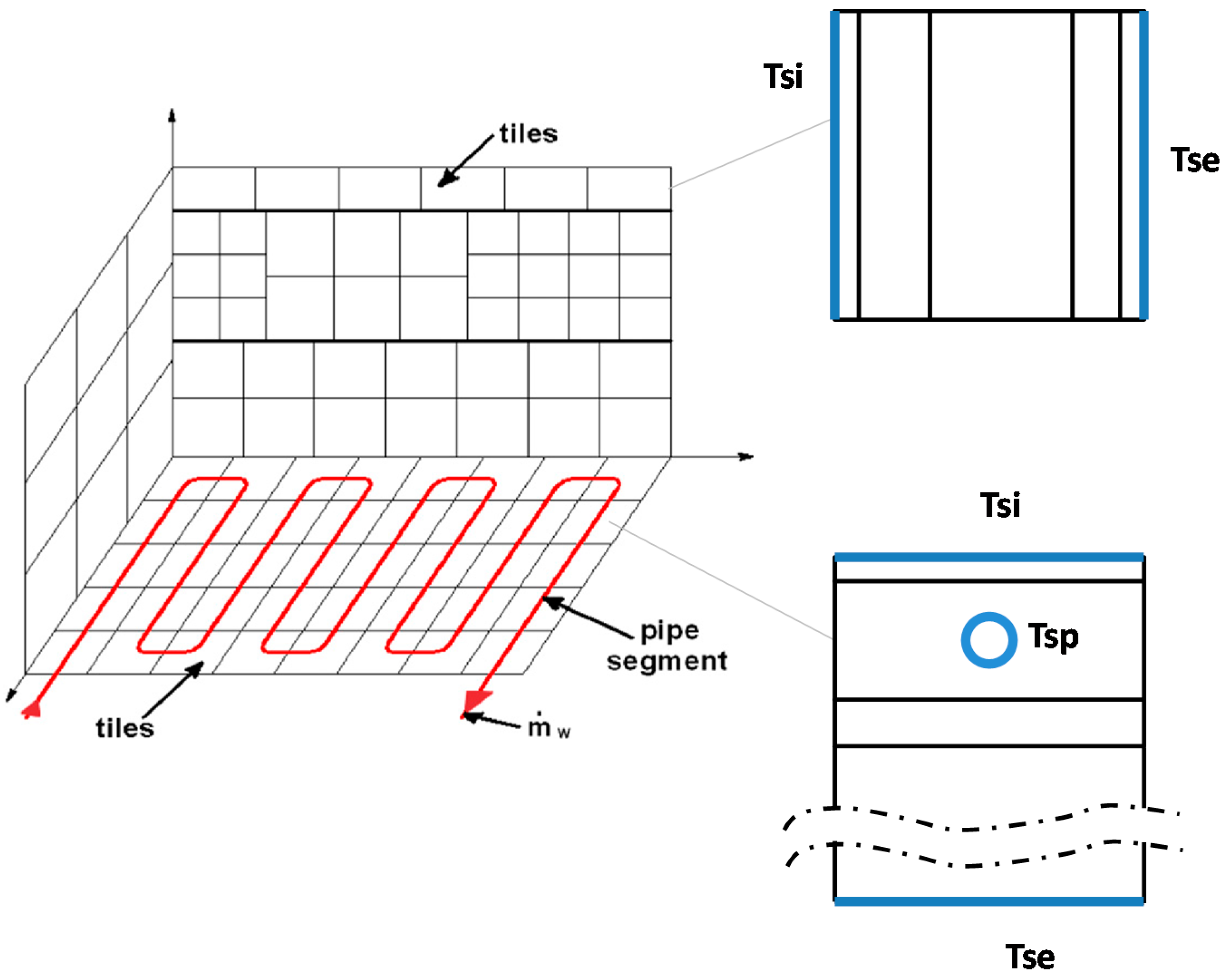
The simulation of the dynamic behaviour of the considered radiant systems in different kinds of buildings has been carried out with the model DIGITHON [
23]. This numerical model performs the detailed simulation of the dynamic behaviour of water-based surface heating and cooling systems. In the model DIGITHON, each surface of the room (containing pipes or not) is divided into elements named tiles (
Figure 1); an overall heat balance is carried out for each element.
To solve the dynamic conduction within the structures the “response factor” technique is used [
24,
25]. In the present work the heat transfer response factors are calculated by using the commercial software HEAT2 [
26], which is based on the Finite Difference Method (FDM). Three simulations must be performed to describe the thermal conduction in a building structure with embedded pipes. In each simulation a triangular impulse of temperature is given on the inner surface, on the outer surface and on the internal surface of the pipes, thus the resulting heat flows on the three surfaces are recorded. After normalization, for a generic trend of temperature on the inner surface of the building structure, on the outer surface of the building structure and on the internal surface of the pipe, the response factor can be used, by superposing of effects, to calculate the specific heat fluxes on the three considered surfaces. More details about this method, included an example showing its accuracy, can be found in [
27]. In case of building structures without embedded pipes, two simulations with triangular input have to be performed.
The convective heat flux for the
j-th general surface element
qc,j is expressed as:
where
Tf,j is the air temperature of the room (for the inner surface elements), the air temperature of the adjacent room (in case of internal walls) or the sol-air temperature (in case of outdoor surface). As for the air temperature, it can be assumed to be uniform when the room is less than 3 m height both in heating [
28] and in cooling conditions [
29] for radiant systems as well as in a wide range of situations that have been confirmed by other studies [
30].
As for convective heat transfer coefficients, a recent review [
31] shows that the most reliable analyses are those based on measurements in real size test rooms. In particular, as shown in [
23], constant values can be considered for the convective heat exchange coefficients. For this purpose convective heat exchange coefficients have been assumed constant in the calculations.
As for the radiative heat exchange, assuming near-black surfaces, in the infrared with small temperature differences the mutual radiation with another surface can be written as:
Since the surface discretisation is fine enough, in the model view factors
Fj-k are calculated in a detail way, as shown in [
27].
Shortwave radiation entering from glazing elements has to be summed on the right side of Equation (2) as well as the internal radiant gains. As demonstrated in detail in [
27] for cooling conditions and in [
32] in heating period, there is no difference in the overall balance when considering solar radiation in detail or when it is assumed to be uniformly distributed. Hence, the solar radiation entering the room in the present work is considered as uniformly diffused.
For the room air, the following equation can be written as:
where flow rates will enter at a given temperature (the external temperature for infiltration or a known inlet temperature for mechanical ventilation) and will leave at room temperature.
A similar equation can be written for the water inside each pipe segment. In this case, due to the discretisation, the temperature difference between two adjacent building elements can be considered very small, thus assuming a linear trend of the temperature in each building element. The representative water temperature is the outlet temperature of each element. Under these hypotheses the equation for the water can be written as follows:
where
Tw,i and
Tw,o are, respectively, the inlet and outlet temperatures in the pipe element. As for the water convection heat transfer coefficients inside the pipes correlations of literature are used [
33].
All equations are linear, therefore the model can be expressed as a product of matrices which provides as results the inner side temperature and the heat flow of each surface element, the air temperature, and the return water temperature of the radiant system.
In the present work the FDM was also used to find the average value of the water temperature in the pipes of the radiant floor system which gives, in steady state conditions, a useful heat flux towards the heated room equal to the thermal losses in design conditions for heat transmission through the building structures, for infiltration and ventilation [
34].
4. Results
The software DIGITHON provides, in the case of ideal convective system, the thermal power needed in the time step to get the required air temperature. This means that the air temperature is fixed and heating is needed only if the air temperature could go below 20 °C as calculated by the thermal balance. If the thermal balance leads to air temperatures greater than 20 °C the air temperature is calculated as a result of the thermal balance. As results the surface temperatures are provided and, hence, the mean radiant temperature, as well as the operative temperature, can be calculated. The heating system has been considered to work constantly 24 h, i.e. no overnight set-back has been assumed. The seasonal energy required by the ideal convective heating system has been named Qid.
When the simulation regards the radiant system, the inputs are the supply water temperature and the mass flow rate in each circuit, and the thermal balance gives as output the return temperature of the water; in this way the energy delivered/absorbed by the water in the time step can be evaluated, as well as the surface temperatures and, hence, the mean radiant and operative temperature. As already mentioned, the control system has been supposed to be on-off with a set-point of 20 °C and a dead band of ±0.5 °C. This means that if the temperature of the room in the time step is lower than 19.5 °C the water circulates in the circuits with a defined supply temperature which could be fixed or variable as a function of external temperature. If the air temperature reaches 20.5 °C the water stops circulating in the circuits and the temperature fluctuates depending on the thermal balance of the room without any active system working in that time step. As for the circuits in the room either all of them work or they do not operate, hence no zone control has been set since the room has been considered as an open space. From the hydronic point of view no other assumptions have been considered, such as a tank or a limiting power supplied by the generator, except for the water volume and related thermal capacity in the circuits in the room. The seasonal energy required by the water embedded heating system has been named Qw.
The on-off control between 19.5 °C and 20.5 °C has been chosen based on a survey provided to companies producing radiant systems in Italy. All producers declared that in flats on-off regulation is the standard control strategy and that PI or PID control is only installed in single family houses due to the high costs of this latest technology.
4.1. Radiant Systems Efficiency
The hourly values of the energy provided as results of the simulations performed by DIGITHON permit the evaluation of the efficiency of the radiant system. Considering the seasonal energy
Qid of an ideal convective system and the seasonal energy provided to the radiant system
Qw, the efficiency of the radiant system can be defined as:
This is a joint embedded and control efficiency since it takes into account the losses of the radiant system behind the pipes as well as the effects of the control system. In
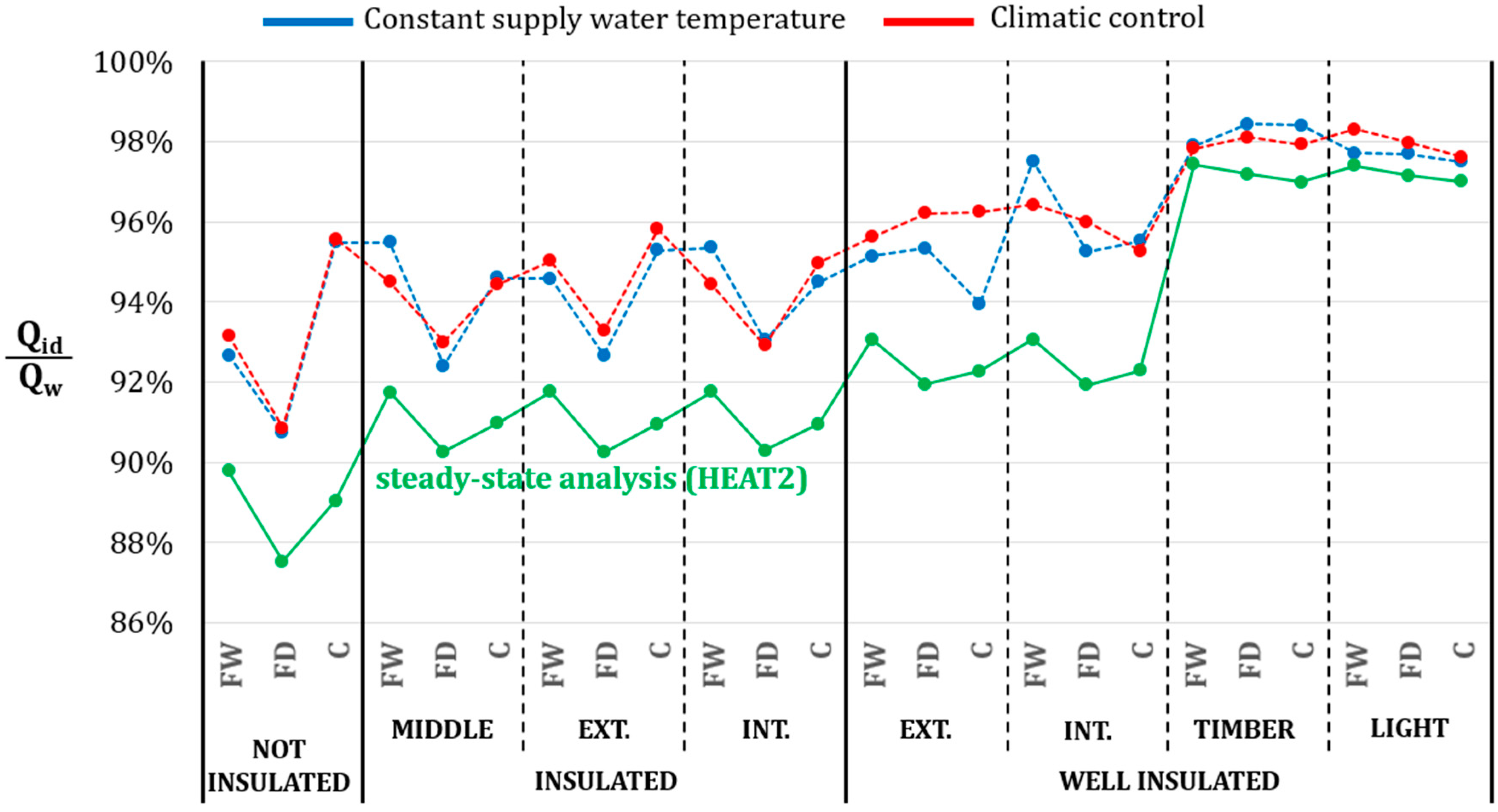
Figure 6 the results obtained for the combination of eight building structures, three radiant systems, and two supply water temperature control modalities are represented. As already explained, these efficiency values are calculated along the whole heating season and hence they include the thermal inertia of the building structures, influence of solar and internal gains, the way the water circulating in the circuit is controlled as well as the heat losses in the room behind the radiant system. Since it is a combination of all these factors, it is not possible to split among a control efficiency and an embedded efficiency but they have to be considered together.
In the same figure, the steady-state embedded efficiency calculated through HEAT2 is represented in green colour. These efficiency values take into account only the geometry and the thermal properties of the building structure where the radiant system is placed and proper boundary conditions. Considering the useful thermal power φ
u towards the heated space and the thermal losses φ
l towards the adjacent space, the embedded efficiency in steady-state conditions of the radiant system can be calculated as:
The following boundary conditions were fixed: room temperatures equal to 20 °C, convective heat transfer coefficient on the surfaces according to
Table 6, adding the radiant heat transfer coefficient on the surfaces equal to 5.5 W m
−2 K
−1, water temperature according to the specific design heat load for each case (
Table 4).
In order to maintain the same comfort conditions (i.e. same operative temperature), the radiant simulations were repeated reducing the air temperature set-point compared to the convective ideal simulation. As already mentioned, the set-point was chosen in such a way that the resulting mean value of the operative temperature in the point P in the period from December to February was the same of the mean value of the ideal convective simulations with set-point of the air Tair = 20 °C. This way an iterative process has been carried out for each single case in order to match the same operative temperature. The period from December to February has been chosen to evaluate the mean value of the operative temperature, because in the insulated building the average temperature in mild months is quite high, the heating system works rarely and it is difficult to compare buildings under the same operating conditions. In fact the heating energy need in the period December-February is, depending on the insulation level, from 75% to 90% of the total heating energy need of the buildings.
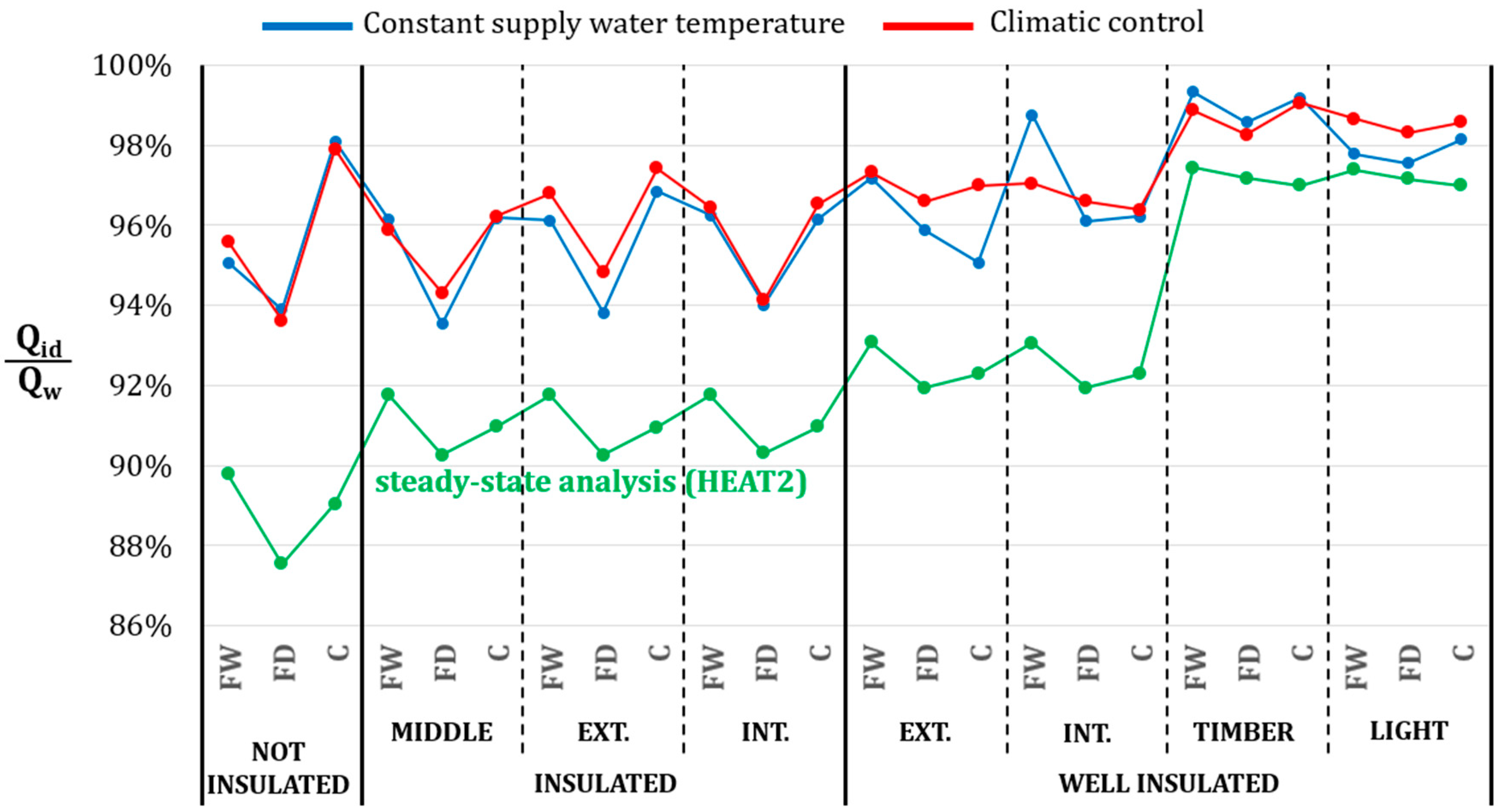
The embedded and control efficiency values for the radiant systems have been calculated via Equation (5). The results are shown for the period December-February (
Figure 6), as well as for the whole season (
Figure 7). As a matter of fact, the first value shows the results under the same indoor conditions (operative temperature), the second one gives an idea on the embedded and control efficiency over the whole season. In
Figure 6 and
Figure 7 also the embedded values which can be calculated in steady state conditions by using Equation (6) with results of FDM are represented. This comparison has been carried out since the embedded emission according to EN 15316 [
37] has to be calculated in steady state conditions as the ratio between the useful thermal input in the indoor environment and the overall power delivered by the water in the pipes. Even though they are calculated in steady state conditions they are then used in the energy performance of a building on a monthly or seasonal base. The analysis of EN 15316 will be considered again later, at the end of this paragraph.
As can be seen, the red line of the climatic control is on average slightly above the blue line of the constant supply temperature control modality. In well-insulated light buildings the efficiency is almost the same (98–99%) regardless the type of radiant system used. These buildings present 2% higher efficiency compared to masonry structures; with these last structures there is no difference among radiant systems in climatic control strategy, while with constant temperature the wet floor performs slightly better. The results of well-insulated buildings of the period December–February (
Figure 6) are very similar to the ones related to the whole season (
Figure 7), since the energy evaluated in this period takes into account 90% of the heating demand of the whole season.
In non-insulated buildings and in insulated buildings usually the dry floor radiant system performs slightly worse than both the wet floor and the ceiling system (about 2%). In these cases when considering the whole season instead of the period December–February there is a 2% difference in the embedded and control efficiency.
The interesting aspect is that the embedded and control efficiency calculated via dynamic simulations (Equation (5)) is higher than the embedded efficiency calculated via steady state conditions (Equation (6)). In light well-insulated structures the embedded and control efficiency of dynamic simulations is 1.5% better than the embedded efficiency estimated via FDM (1% if considering the period December–February, 2% if the whole season). In masonry well-insulated buildings the embedded and control efficiency of dynamic simulations is 3.5% better than the embedded efficiency estimated via FDM with constant supply temperature (3% if considering the period December-February, 4% if the whole season), while dynamic simulations provide 4.5% better embedded and control efficiency than the embedded efficiency estimated via FDM in the case of climatic control (4% if considering the period December–February, 5% if the whole season). In insulated buildings the difference is almost 4% regardless to the water supply temperature, while for non-insulated buildings the difference is 6%. It is useful to highlight that the efficiency calculated via FDM is evaluated with constant indoor temperature and in steady-state conditions, as usually done by producers of radiant systems and practitioners and, therefore, depends only on the difference between water temperature and room temperature and on the thermal conductivity of the materials of the various layers, but not on their thermal capacity. In dynamic conditions the situation is completely different, both for the water inside the pipes and for the boundary conditions. For most of the time the heat load required by the heated room is lower than the design heat load, and hence warm water is not continuously flowing in the pipes of the radiant system. The changing indoor conditions and the consequent on-off operation of the radiant system lead to a complex mechanism of absorption and release of heat in the different layers of the floor and the percentage losses results lower than in steady-state conditions. This means that part of the heat delivered by the pipes is absorbed by the layer containing them and, when water stops flowing, part of this becomes useful gain instead of backwards loss.
As regards the efficiency values which can be found in the standards, the old version of EN ISO 15316-2-2007 [
37] recommends to use an embedded and control efficiency value which is equal to 90% for the wet floor and ceiling systems (
ηctr = 0.95,
ηemb = 0.94) considered in this study and 91.3% for the dry floor system (
ηctr = 0.95,
ηemb = 0.955). No difference in the efficiency values in the old version of the standard is considered to take into account the different insulation level and thermal inertia of the building.
In the last version of the standard EN ISO 15316-2-2017 [
38], the calculation method to evaluate the energy required by a heating or cooling system is only based on internal temperature variations, while the calculation method based on efficiency values was removed. Therefore, in the present work besides efficiency values, also the internal temperature variation was calculated from the results of the simulations for the period from December to February.
As can be seen in
Table 8, the current standard overestimates the losses of the radiant systems: in the non-insulated case the difference is about 0.7 °C for the radiant floor and 1.5 °C for the ceiling. In insulated buildings the difference is 1.1°C in insulated buildings and 1.4 °C for the radiant ceiling. In well-insulated masonry buildings the difference is 1.2 ÷ 1.5 °C compared to the existing standard temperature variation for the radiant floor and 1.2 °C for the radiant ceiling. In well-insulated buildings with light structures the difference is about 1.7 °C ÷ 2.0 °C for the radiant floor, as well as for the radiant ceiling. These values are conservative since the calculation has been limited in the period December–February which is the one which provided the lowest efficiencies in terms of losses and hence the greatest values of the temperature difference Δ
Ti,emb + Δ
Ti,ctr.
4.2. Energy Analysis
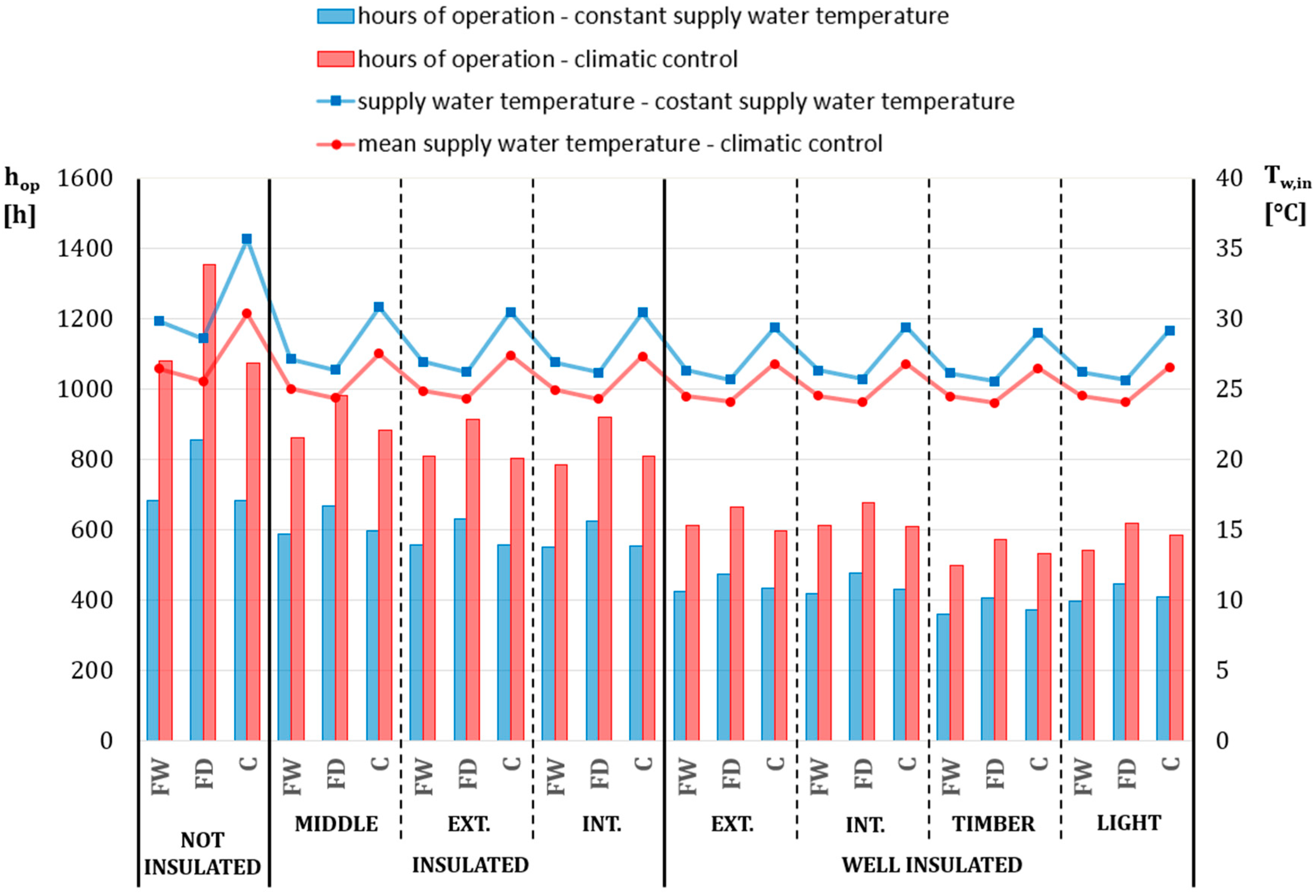
In addition to the embedded and control efficiency, the overall energy consumption should also be evaluated. Concerning the supply water temperature control modality, the climatic control has the undeniable advantage of reducing its seasonal mean value of about 4 °C in non-insulated buildings, 2.5 °C in insulated buildings, and 2 °C in well-insulated buildings (
Figure 8). The ceiling systems need higher water temperatures than floor systems because of the lower convective heat transfer coefficient and of the smaller active surface; for this reason the ceiling systems show the greatest temperature reductions among the three kinds of radiant systems when going from the fixed temperature to variable supply temperature related to outside air (climatic control strategy). As regards the operation time, the climatic control obviously shows an increase, which is equal to 58%, 46% and 41% for the non-insulated, insulated and well-insulated buildings respectively.
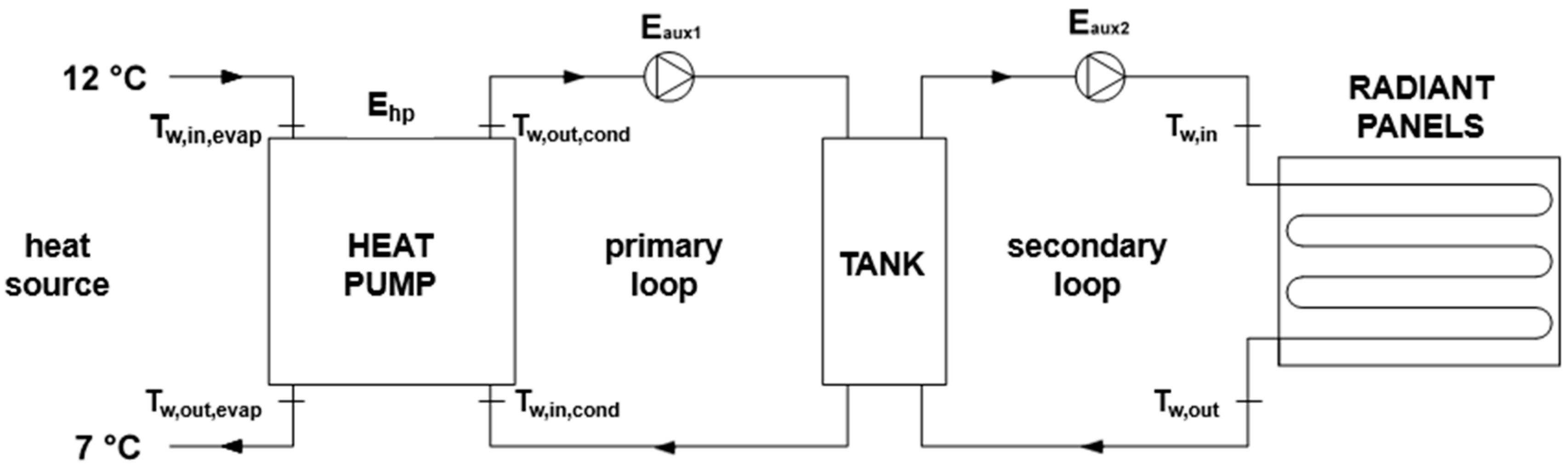
A simplified evaluation of the energy consumption of the entire heating system was done considering a water-to-water heat pump as generator, a primary loop, and a secondary loop with their pumps (
Figure 9).
The electric energy consumption of the heat pump was estimated considering a heat source constantly at 12 °C and a temperature difference at the evaporator of 5 °C (water source temperature from 12 °C to 7 °C). The nominal conditions in
Table 9 from a commercial datasheet were considered to evaluate the coefficient of performance (COP).
For evaluating the COP of the heat pump the ideal coefficient of performance of a Carnot cycle has been used:
where the condensing and evaporating temperatures of the cycle have been evaluated as follows:
By using Equations (3)–(5), in nominal condition the ideal Carnot cycle gives
COPid,nom = 9.41. At each time step of the simulations the ideal coefficient of performance
COPid was calculated considering the mean value of the water temperature in the condenser equal to the supply water temperature
Tw,in of the radiant panels. The COP of the heat pump was then estimated as follows:
At each timestep the electric energy consumption of the heat pump
Ehp can be calculated as:
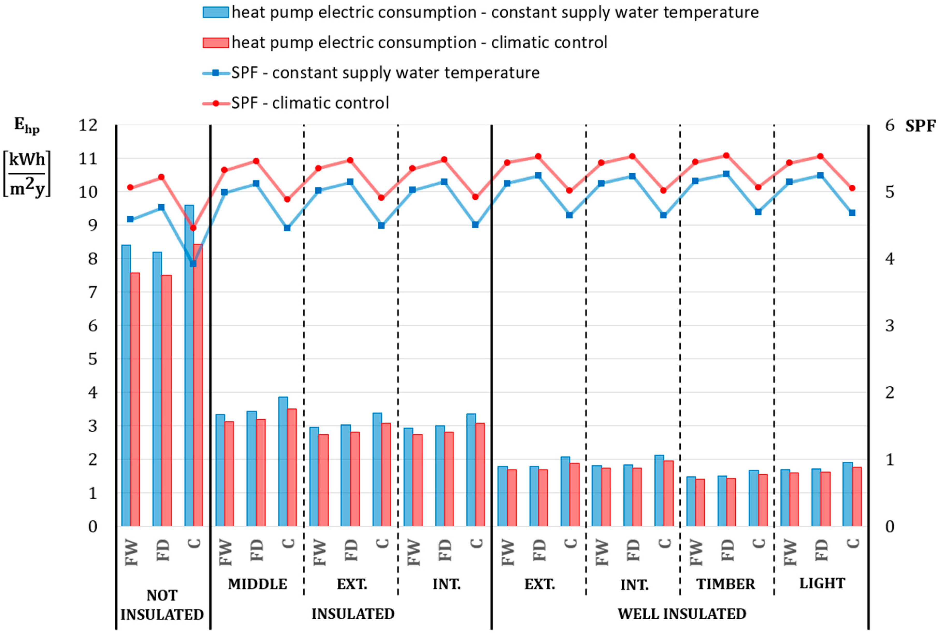
From the seasonal thermal energy and the corresponding electric consumption, the mean value of the COP can be calculated. This is called seasonal performance factor, SPF, and its value can be seen in
Figure 10 (right axis) together with the electric energy require by the heat pump (left axis).
The higher SPF which can be achieved with the climatic control of the supply water temperature makes the heat pump electric consumption lower, but also the electric consumption of the auxiliaries should be evaluated. As already seen in
Figure 8, the number of hours of operation of the pump of the secondary loop is much higher in the case of climatic control instead of constant supply water temperature. The pressure drops of each combination of radiant system and building type were calculated and the electric power of the pump was then evaluated from the chart of a common high efficiency pump for domestic use. For the primary loop the number of hours of operation of the pump was calculated from the seasonal thermal energy need and the nominal thermal power of the heat pump.
The resulting total electric energy consumption
Etot can be seen in
Table 10, where also the electric energy consumption of the heat pump
Ehp, of the primary pump
Eaux,1 and of the secondary pump
Eaux,2 are listed.
If the generator of the heating system is a heat pump and the radiant circuits are properly designed, the increase of the operation time of the secondary loop with climatic control instead of constant supply water temperature is in any case balanced by the reduction of the consumption of the heat pump due to the lower water temperature. Considering the ceiling system, the climatic control modality ensures a reduction of the total electric energy consumption of about 11%, 8%, and 7% for the non-insulated, insulated and well-insulated buildings, respectively. With the floor systems the reduction is about 8%, 5%, and 4%, respectively.
4.3. Overtemperature Analysis
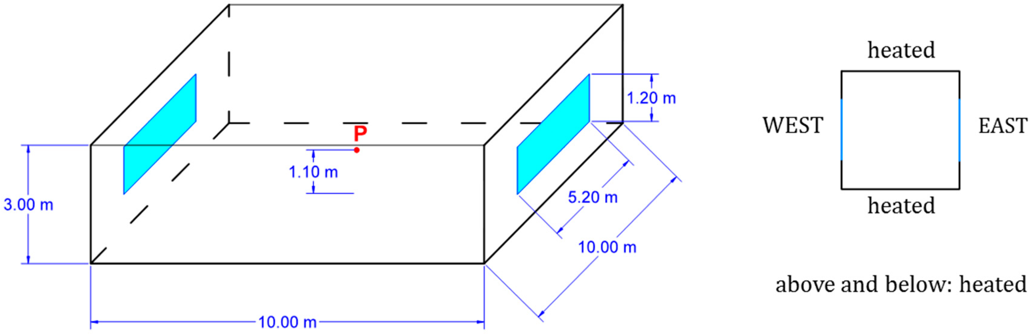
An analysis was carried out on the operative temperature in the point P (
Figure 2) in the period from December to February, considering the degree hours criteria described in Annex F of EN 15251 (2007) [
39]. A temperature range was defined and the degree hours outside the upper boundary of the range (
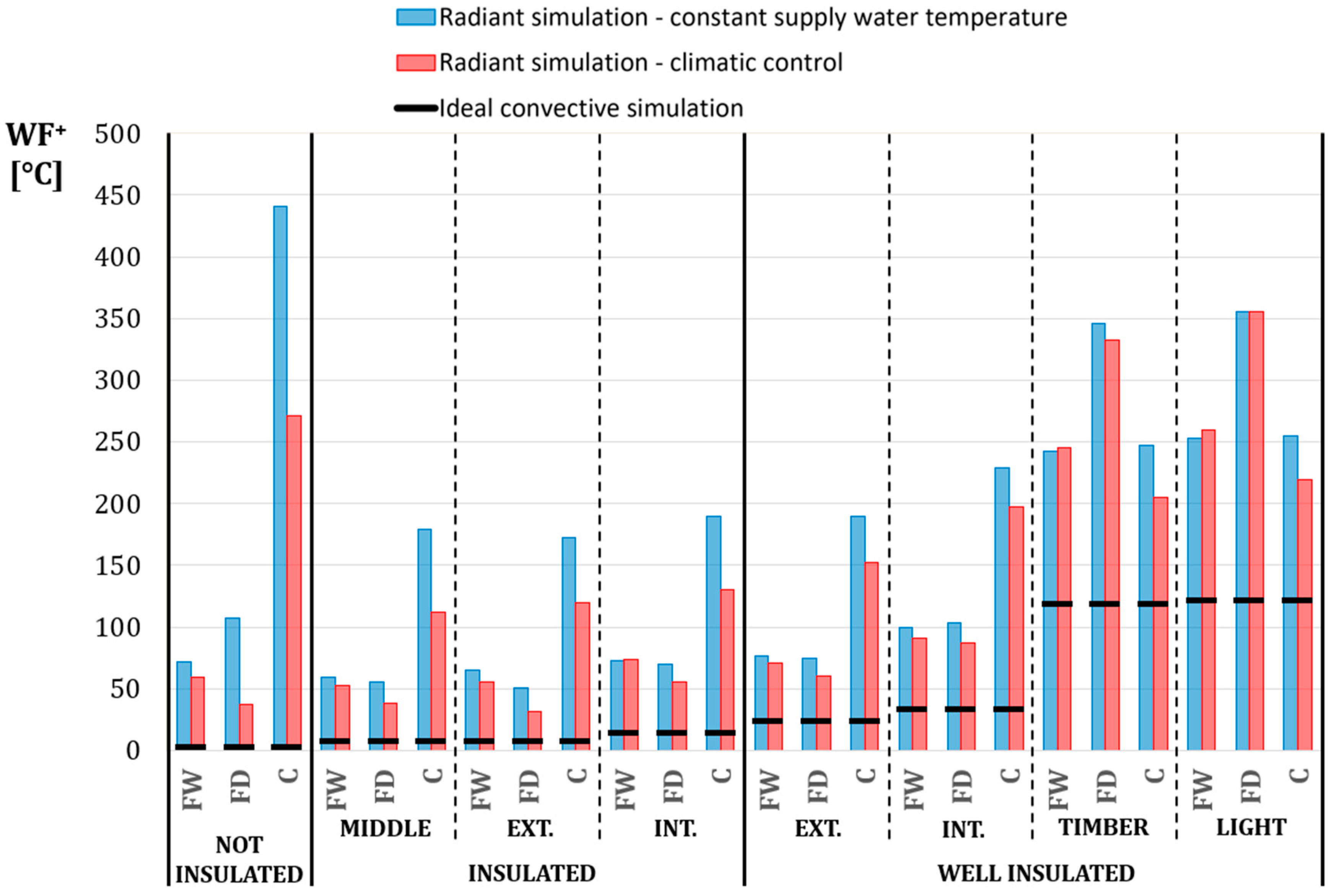
Tul) was used as a performance indicator of the building for the heating season in relation to the overtemperature. The weighting time for overtemperature WF
+ can be calculated as:
Since the simulations have been performed maintaining in the convective ideal case the air temperature constant at 20 °C, the operative temperature differs in all cases. Hence, a specific range was defined for each radiant case, centred on the mean value of the operative temperature, which is the same of the ideal convective cases, and with an amplitude of 1.0 °C (i.e. ±0.5 °C). A small band was chosen, with the same amplitude of the on-off thermostat, since the purpose was not the evaluation of comfort conditions, but simply the evaluation of the periods with the operative temperature rising outside the control band of the air temperature and the comparison of these periods with different envelopes and type of radiant systems, as well as the comparison between the building with the radiant systems and the same building with an ideal convective heating system. A larger band was not suitable for a fully exhaustive evaluation for this purpose, since it was found that, in the worst cases (well-insulated timber envelope and light envelope with dry floor system), the operative temperature exceeded more than 1.5 °C its mean value for only about 3% of the time, i.e. no discomfort has been found for overheating in all the cases.
In
Figure 11 the WF
+ calculated from the results of the radiant simulations are represented. As can be noticed, the constant supply water temperature control modality always gives a higher WF
+ than the climatic control modality, except for the well-insulated buildings, where the WF
+ are similar. The ceiling systems present a WF
+ which is, on average, more than five times the WF
+ of the floor systems in the non-insulated building and 2.5 times in the insulated and well-insulated masonry buildings. In the well-insulated lighter buildings the dry-floor system presents the highest WF
+, almost 1.5 times the WF
+ of the wet-floor and ceiling systems.
It is interesting to notice that the 50% of the WF+ of the well-insulated light buildings can be already found in the ideal convective simulations. This percentage decreases to 27% for the well-insulated masonry buildings, 12% percent for the insulated buildings and only 2% for the non-insulated buildings. In a convective system controlled with an on-off band like the simulated radiant systems, these percentages would certainly be higher, showing that the problem of overtemperature in well-insulated buildings is not strictly related to the radiant system itself, but it is inevitable especially in the case of light structures (even in ideal conditions); secondly, the control modality may affect the overtemperature.
In
Figure 12 the value WF
+/h
+ of the overtemperature is represented; h
+ is the number of hours which contribute to the overall value of WF
+, i.e., the number of hours in which the operative temperature exceeds the threshold value defined; this parameter can be named overtemperature intensity. In the insulated buildings the overtemperature intensity is the same of the ideal convective cases, except for the constant supply water temperature ceiling systems which show much higher values. The well-insulated masonry buildings with wet-floor radiant system show an overtemperature intensity lower than that of the ideal convective system. The same occurs in the well-insulated light buildings for the wet floor radiant systems and also for the ceiling systems, but not for the dry-floor systems.
5. Conclusions and Discussion
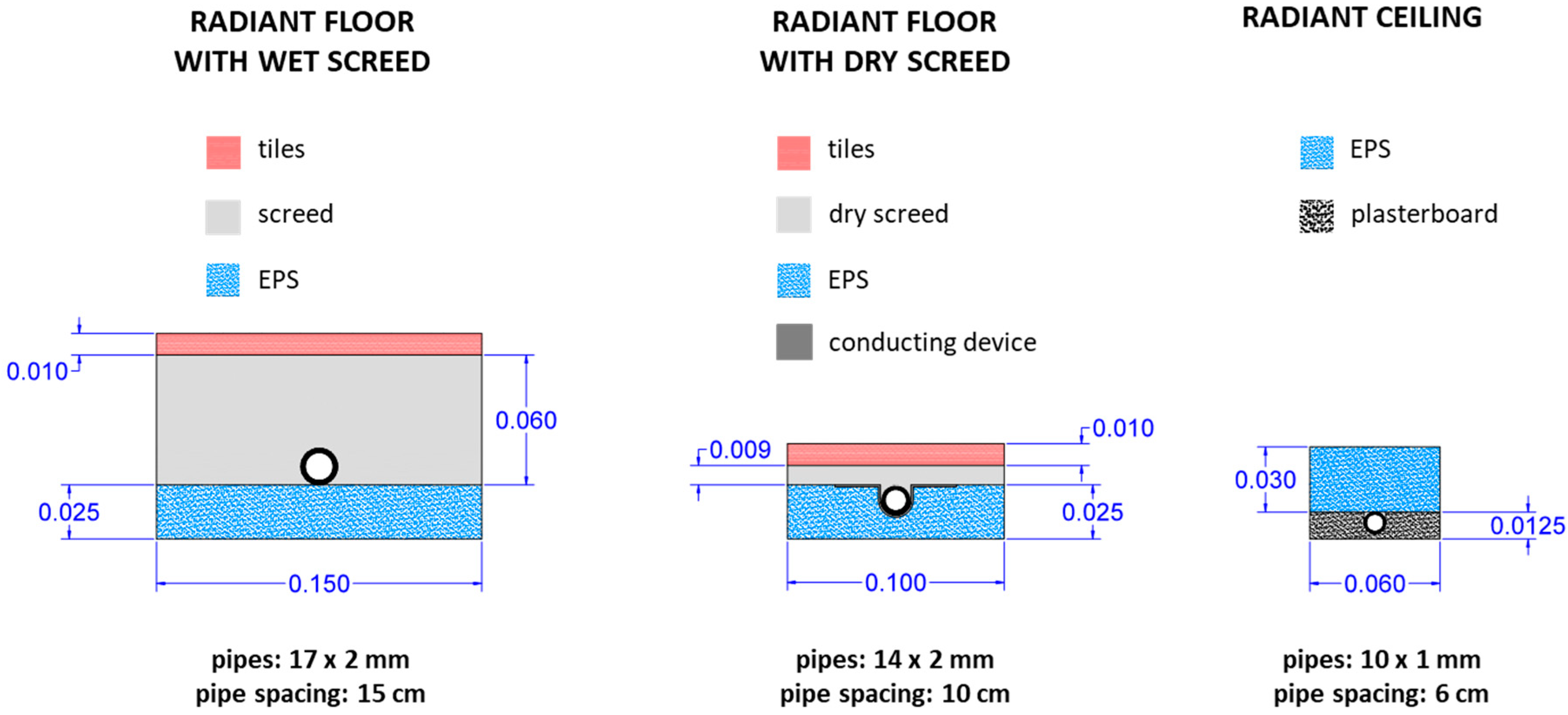
The work carried out is based on simulation of a room which represents an intermediate multi-story flat of about 100 m2 where three types of radiant systems have been modelled: two radiant floors (one with usual pipes embedded in wet screed and one with low thickness dry screed) and a radiant ceiling. The work looks at the performance of these systems in heating conditions with three insulation levels of buildings: no insulation, insulated building and well-insulated building. Three types of insulated buildings (with internal, intermediate, and external insulation) and four types of well-insulated buildings (masonry with external and internal insulation, timber structure, and light structure) have been analysed. Dynamic simulations of the radiant systems with fixed temperature and with variable temperature according to outdoor temperature have been compared with an ideal convective dynamic simulation.
Results have been analysed in terms of control and embedded efficiency of the radiant system, energy performance of the radiant system with a water to water heat pump at fixed source temperature, as well as possible overtemperature.
About the embedded and control efficiency, the climatic control strategy performs slightly better than the constant supply temperature control modality. In well-insulated light buildings the efficiency of the two control strategies is almost the same (98–99%) regardless of the type of radiant system used. These buildings present a 2% higher efficiency compared to masonry structures, with these last structures the different types of radiant systems show the same efficiency value in case of climatic control strategy, while with constant temperature the wet floor performs slightly better. In non-insulated buildings and in insulated buildings usually the dry floor radiant system performs about 2% less than both the wet floor and the ceiling system (which present circa 96% of efficiency).
The embedded and control efficiency calculated via dynamic simulations has been compared to the embedded efficiency calculated via steady state conditions. In light well-insulated structures the embedded and control efficiency of dynamic simulations is 1.5% better than the one estimated via FDM. In masonry well-insulated buildings the embedded and control efficiency of dynamic simulations is 3.5% better than the one estimated via FDM with constant supply temperature, while climatic control simulations provide 4.5% better embedded and control efficiency than the one estimated via FDM. In insulated buildings the difference is almost 4% regardless to the water supply temperature, while for non-insulated buildings the difference is 6%.
The old version of the standard EN15316-2-2007 [
37] provides for the embedded and control efficiency 90% for the wet floor and ceiling systems and 91.3% for the dry floor system. The dynamic simulations provide for the wet floor and the ceiling as average 96% in non-insulated buildings, in insulated buildings and in masonry well-insulated buildings, 98% in well-insulated buildings with light structures. The dry floor presents an embedded and control efficiency of about 93% in non-insulated buildings and in insulated buildings, 95% in masonry well-insulated buildings, and 98% in well-insulated buildings with light structures.
Referring to the new version of the standard 15316-2-2017 [
38], the current values of the temperature difference Δ
Ti,emb + Δ
Ti,ctr are higher than the ones calculated in the present work. Based in the dynamic simulations, the suggested values for the joint embedded and control temperature differences are the ones reported in
Table 8, which should substitute the existing default values. Moreover, the efficiency calculated in transient conditions is higher than the efficiency calculated under steady state conditions. This result is because, over the season, the radiant systems work for some hours and then they switch off. Part of the thermal energy embedded in the structures is not lost when the water stops flowing in the pipes, but it is later released to the room.
When considering the overall energy consumed by a water to water heat pump (including the auxiliaries) the increased amount of hours of pumping in the case of variable temperature is counterbalanced by the higher COP of the heat pump, which increases when the supply temperature decreases; overall the climatic control leads to 5–6% better performance in floor heating systems and 7–8% better performance with radiant ceilings. Overall the radiant ceiling consumes always more than the two floor systems due to the higher supply temperature (about 11% in the case of variable temperature and 15% in case of fixed temperature). Of course, the higher the insulation the higher the performance, hence, the light structures perform better than the masonry structures due to the lower U-values.
Looking at long-term comfort evaluations results, no particular problem has been found in the period from December to February according to EN 15251 category II. The analysis carried out was mainly related to check the overtemperature, i.e., when the temperature is above the set-point temperature plus the dead band fixed in 0.5 °C in the present work. The results show that overtemperature rises when the insulation increases. In masonry structures radiant ceiling has always the highest values of WF+, especially in case of constant supply temperature. This is due to the higher water temperature supply, although the radiant structure is light. In well-insulated light structures the dry floor shows the highest overtemperature. Anyway, it has to also be underlined that in the ideal convective system simulations the overtemperature is comparable with the ones of the radiant systems simulations. In particular when dividing WF+ by the number of hours when the overtemperature occurs h+, the intensity of overtemperature (WF+/h+) shows that the results of radiant systems and ideal convective case are of the same magnitude. This means that, with radiant systems the amount of hours when the overtemperature occurs, h+ is higher, but the intensity of the overtemperature is similar than in the ideal convective case.
Resuming the results, the work carried out shows that in general the better the quality of the envelope the better the overall performance of the radiant system. Evaluating the efficiency in dynamic conditions leads to higher efficiencies compared to steady state conditions, former standard EN 15316-2-2007 and also the new standard EN15316-2-2017 and new suggested values are provided. Working at variable temperature leads to lower consumptions compared to fixed supply temperature over the season. No problems of comfort have been found in the period from December to February. Overtemperature effects are not especially due to radiant system, but they also happen in any case with ideal convective systems. As with all emission systems, the radiant systems may lead to higher overtemperature effects, but the effect is evident in terms of higher amount of hours when the overtemperature happens rather than too high temperatures because of the radiant system operation.
In general, the radiant ceilings perform worse than radiant floor systems in heating conditions and there is no evidence that dry floor systems perform better than wet screed systems in all the types of buildings regardless of the level of insulation and thermal inertia.
As a final remark, it has to be underlined that it would be interesting to analyse the same building in cooling conditions, where the radiant ceiling could work better than the radiant floor system. Moreover, the work which has been carried out here considers a unique room; a further interesting study would be to analyse different rooms, i.e., looking in detail at the distribution of the inner space and checking the different possible control strategies.


