Transfer Learning with Deep Recurrent Neural Networks for Remaining Useful Life Estimation
by
 , , and
Ansi Zhang
1,2, 
Honglei Wang
3,
Shaobo Li
1,4,*,
Yuxin Cui
2,
Zhonghao Liu
2,
Guanci Yang
1 and
Jianjun Hu
2,4,* 1
Key Laboratory of Advanced Manufacturing Technology of Ministry of Education, Guizhou University, Guiyang 550025, China
2
Department of Computer Science and Engineering, University of South Carolina, Columbia, SC 29208, USA
3
Guizhou Provincial Key Laboratory of Internet Collaborative intelligent manufacturing, Guizhou University, Guiyang 550025, China
4
School of Mechanical Engineering, Guizhou University, Guiyang 550025, China
*
Authors to whom correspondence should be addressed.
Appl. Sci. 2018, 8(12), 2416; https://doi.org/10.3390/app8122416
Submission received: 14 September 2018
/
Revised: 7 November 2018
/
Accepted: 10 November 2018
/
Published: 28 November 2018
(This article belongs to the Special Issue Fault Detection and Diagnosis in Mechatronics Systems)
Abstract
:Prognostics, such as remaining useful life (RUL) prediction, is a crucial task in condition-based maintenance. A major challenge in data-driven prognostics is the difficulty of obtaining a sufficient number of samples of failure progression. However, for traditional machine learning methods and deep neural networks, enough training data is a prerequisite to train good prediction models. In this work, we proposed a transfer learning algorithm based on Bi-directional Long Short-Term Memory (BLSTM) recurrent neural networks for RUL estimation, in which the models can be first trained on different but related datasets and then fine-tuned by the target dataset. Extensive experimental results show that transfer learning can in general improve the prediction models on the dataset with a small number of samples. There is one exception that when transferring from multi-type operating conditions to single operating conditions, transfer learning led to a worse result.
1. Introduction
Recently, fault diagnosis and health management, including diagnosis and prognosis approaches, have been actively researched [1,2,3,4,5]. Fault diagnosis and health management techniques are widely applied in diverse areas such as manufacturing, aerospace, automotive, power generation, and transportation [6,7,8,9]. Diagnostics is the process of identification of a failure. Prognostics is an engineering discipline focusing on the prediction of the time when a system or a component fails to perform its intended function. In diagnostics, once degradation is detected, unscheduled maintenance should be performed to prevent the consequences of failure. In prognostics, maintenance preparation could be performed when the system is up and running, since the time to failure is known early enough. A major application of prognostics is estimating remaining useful life (RUL) of systems. It is also called remaining service or residual life estimation [10]. Prognostic methods can be grouped into two major categories: data-driven methods, and physics-based methods. The former requires sufficient samples that are run until faults or failures are detected, whereas the latter require an understanding of the physics of system failure progression [11].
In recent years, the data-driven approaches for remaining useful life (RUL) studies [12,13,14,15,16] have been attracting a lot of attention due to their avoidance of dependency on the theoretical understanding of complex systems. However, a major challenge in data-driven prognostics is that it is often impossible to obtain a large number of samples for failure progression, which is costly and labor demanding [11]. This situation can arise for several reasons: (1) industry systems are not allowed to run until failure due to the consequences, especially for critical systems and failures; (2) most of the electro-mechanical failures occur slowly and follow a degradation path such that failure degradation of a system might take months or even years [17]. Several methods have been used to address this challenge. The first approach is accelerated aging by running the system in a lab with extreme loads, increased speed or using imitations of real components which are made by vulnerable materials, so that a failure progresses faster than normal [14,15,16]. Another approach is introducing unnatural failure progression by using exponential degradation to model regular failure progression [18]. Both methods have their own strengths and weaknesses with the capability to represent the failure degradation to a certain level. However, in real-world applications where the condition is very different from the lab environment, these methods are difficult to apply and to obtain good estimation performance.
Recently, deep learning has been shown to achieve impressive results in areas such as computer vision, image and video processing, speech, and natural language processing [19]. Deep learning methods have also been applied to fault diagnosis [20,21,22] and the RUL estimation problem. For the RUL estimation problem, a Convolutional Neural Network (CNN) is applied on a sliding window with multi-times weight and failures height in [23]. However, a major limitation of this work is that the sequence information is not fully considered in the CNN model. To address this issue, a Long Short-Term Memory (LSTM) model was proposed for RUL estimation [24], where the model can make full use of the sensor sequence information and performs much better than the CNN model. Following this success, Convolutional Bi-directional Long Short-Term Memory networks (CBLSTM) have been designed in [25] for RUL prediction, where firstly a CNN is first used to extract robust and informative local features from the sequential input, and then a bi-directional LSTM is introduced to encode temporal information. In addition to these approaches which use the raw input, a Vanilla LSTM neural network model has been used in [26] for RUL prediction, where a dynamic differential technology was proposed to extract inter-frame information and achieved high prediction accuracy. Moreover, an ensemble learning-based prognostic method is proposed in [27], which combines prediction results from multiple learning algorithms to get better performance. However, all these modern deep learning approaches for RUL prediction have a major limitation: they all require the availability of a large amount of training data for training these deep neural networks, while in real-world applications, it is often impossible to obtain a large number of failure progression samples. Therefore, both these deep neural network methods and traditional methods have not addressed the major challenge in data-driven prognostics: the big data of failure samples.
In this paper, we propose to use transfer learning-based deep neural networks for RUL prediction. In recent years, transfer learning has made great progress in image, audio, and text processing to address the data scarcity issue by taking advantage of datasets in related domains. It is widely adopted in the situation where source data and target data are in different feature spaces or have different distributions [28,29]. Transfer learning methods work by learning properties from source data and transfer them to the target data. The source data and target data can be different. But they should be more or less related. Zhong et al. [30] applied the domain separation framework of transfer learning for automatic speech recognition. Singh et al. [31] applied transfer learning in object detection with improved detection performance. Cao et al. [32] used transfer learning for breast cancer histology image analysis and achieved better performance than the popular handcrafted features. These studies showed that transfer learning can make use of both source data and target data to get better performance. In real-world applications of RUL prediction, the scarcity of target data is one of the major challenges in data-driven prognostics as it is often not possible to obtain large numbers of samples of failure progressions. However, we usually have access to a large amount of data of different but approximately related working conditions.
In this paper, we proposed a transfer learning approach with LSTM deep neural networks for RUL prediction. It provides an effective way to address the major challenge in data-driven prognostics. Our contribution in this paper includes:
- (1)
- We developed a bidirection LSTM recurrent neural network model for RUL prediction;
- (2)
- We proposed and demonstrated for the first time that the transfer learning-based prognostic model can boost the performance of RUL estimation by making full use of different but more or less related datasets;
- (3)
- We showed that datasets of mixed working conditions can be used to improve the performance of single working condition RUL prediction while the opposite is not true. This can give good guidance in real-world application where samples of certain working conditions are hard to obtain.
2. Methods
2.1. The Turbofan Engine RUL Prediction Problem and the C-MAPSS Datasets
To verify our transfer learning-based algorithm, we selected the Turbofan Engine RUL prediction problem as the benchmark. The corresponding C-MAPSS datasets (Turbofan Engine Degradation Simulation Datasets) are widely used for RUL estimation [33]. These datasets are provided by the NASA Ames Prognostics Data Repository [34], which contains 4 sub-datasets as given in Table 1. Each sub-dataset consists of multiple multivariate time series, which are further divided into training and testing sets. In the training set, the fault grows in magnitude until the system fails. In the testing set, the time series ends some time prior to system failures.
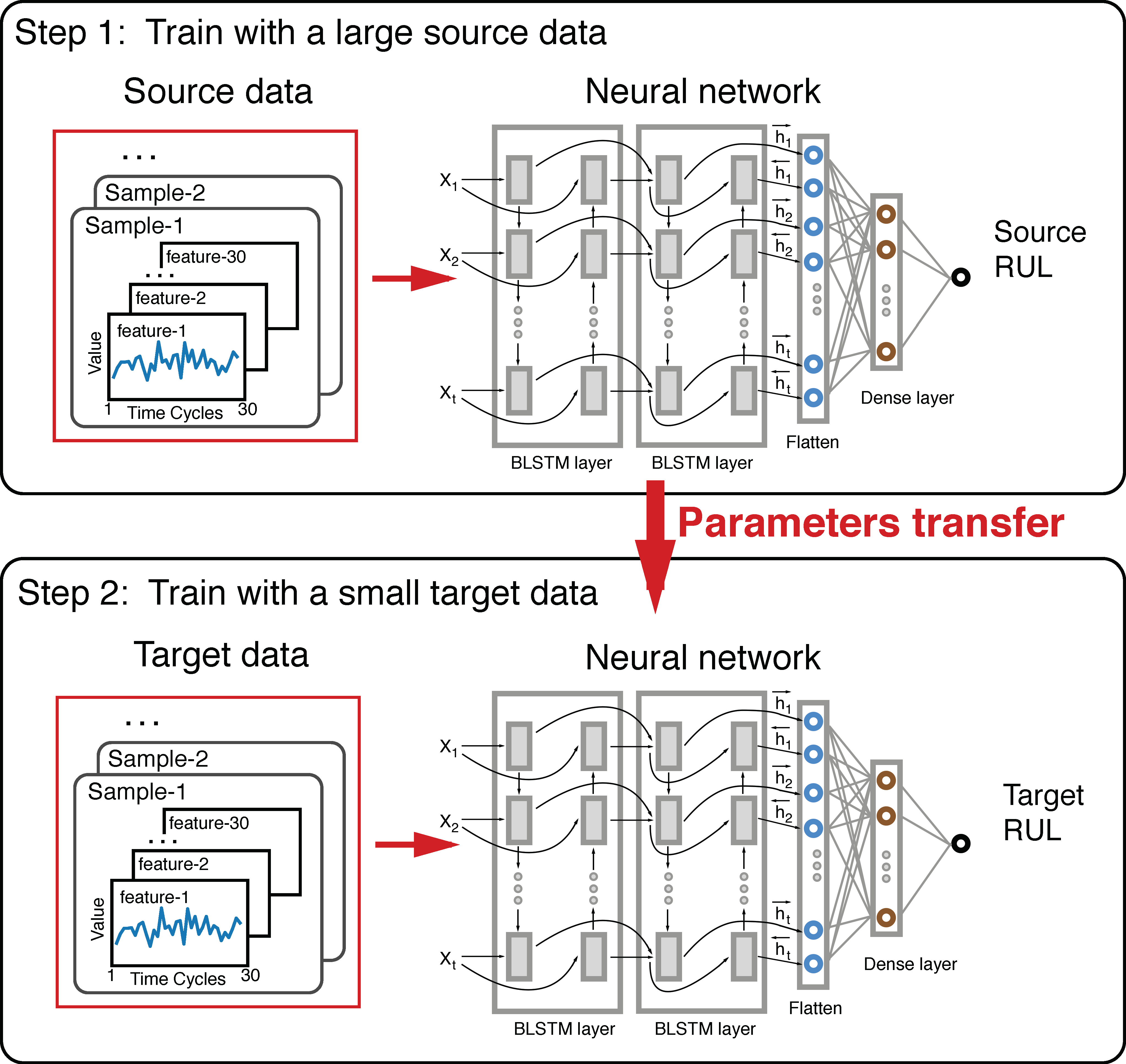
Every trajectory is an engine’s cycle records data. Every cycle record is a snapshot of data taken during a single operational cycle. A single-cycle datum in the C-MAPSS dataset is a 24-dimensional feature vector consisting of 3 operational settings and 21 sensor values. The operating condition settings are altitude, Mach number, and throttle resolver angle respectively, which determine different flight conditions of the aero-engine. In sub-dataset FD001, the engine suffered a failure of a high-pressure compressor with a single operation condition. In sub-dataset FD002, engine suffered a failure of a high-pressure compressor with six operation condition. In sub-dataset FD003, engine suffered a failure of a high-pressure compressor and fan with a single operation condition. In sub-dataset FD004, engine suffered a failure of a high-pressure compressor and fan with six operation condition.
Figure 1 illustrates the standardized operational setting values in every sub-dataset. The operational setting 3 values are stable in FD001 with a single operation condition, just as in FD003. The change and distribution of operational setting values are different between a single operation condition and six operation conditions.
2.2. Transfer Learning for RUL Prediction
Based on the availability of sample labels, transfer learning can be divided into three categories: inductive transfer learning, transductive transfer learning, and unsupervised transfer learning [28]. Inductive transfer learning requires the availability of the target data labels. If the source data labels are available and the target data labels are unavailable, transductive learning should then be used. If both the target data labels and the source data labels are unavailable, then the unsupervised transfer learning should be used. According to the properties of C-MAPSS datasets in which both the target data labels and the source data labels are available, inductive transfer learning is the most suitable approach that we adopted.
Based on what to transfer, transfer learning can be conducted at several levels: instance-transfer, feature-representation-transfer, parameter-transfer, and rational-knowledge-transfer [28]. Instance-transfer aims to re-weight some labeled data from the source domain and then use them in the target domain. Feature-representation-transfer tries to get the good feature representations that can reduce the difference between the source domain and the target domain. Parameter-transfer discovers shared parameters or prior knowledge between the source domain and the target domain. Relational-knowledge-transfer works by mapping the common relational knowledge or some similar patterns from the inputs to the outputs between both domains. According to the properties of the C-MAPSS datasets and experiment conditions, parameter-transfer is selected in our algorithm.
In this research, we apply transfer learning to address one of the major challenges in data-driven prognostics by transferring model parameters learned from the different but approximately related domain with a large amount of source data to the target RUL prediction problem with a small amount of data. The parameter-transfer scheme can be defined as follows:
where , , , , , respectively represent source domain, source samples, source task labels, target domain, target samples, target task labels. , are related or similar domains.
The relationship of the model weights of the source problem and of the target problem can be represented as follows:
Here, , are parameters in the source and the target task, respectively. They have some common parts and some different parts. , are the real outputs. , denote the learning models that map from the sample inputs to the task labels. The parameter-transfer scheme aims to transfer parameters from to by making use of the common parts and fine-tuning the different parts by further training the models in the target task.
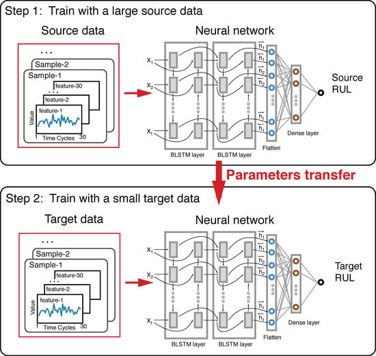
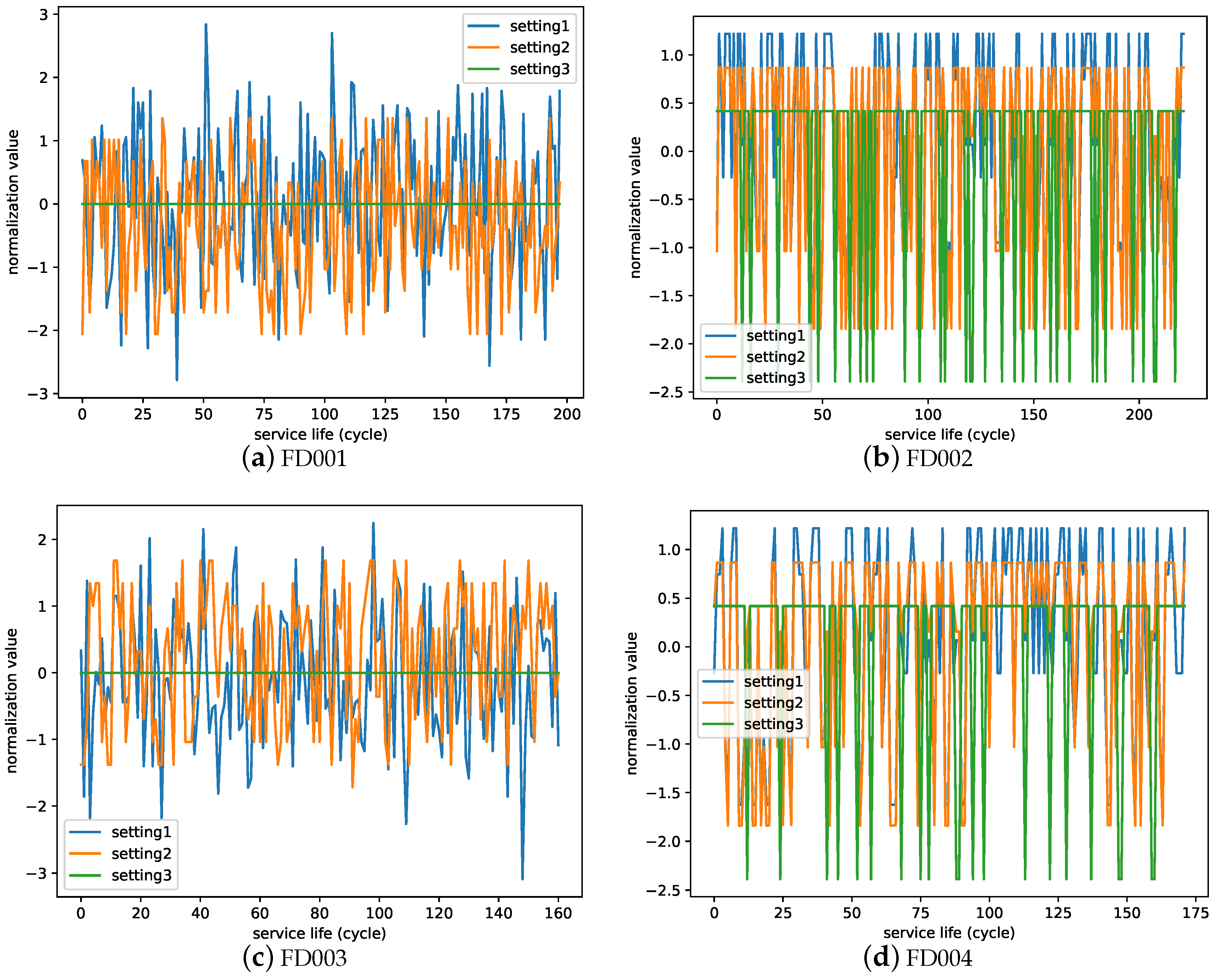
2.3. The Transfer Learning Framework for RUL Prediction
The transfer learning framework is illustrated in Figure 2. The framework is composed of two Long Short-Term Memory (LSTM) networks. The network on the top was trained on the large amount data of the source task. Then the learned model was fine-tuned by further training with the small amount of data from the target task, which is usually a different but related task. In our experiments, it represents the degradation failure under different working conditions.
2.3.1. The BLSTM Neural Networks
To take advantage of the sequential nature of the sensor data in the turbine engine RUL prediction problem, recurrent neural networks (RNNs) are favored due to their ability to capture time-dependent relationships. However, conventional RNNs have the issue of vanishing and exploding gradient problems, which makes it extremely challenging to train such models. To address these issues, Long Short-Term Memory (LSTM), a gated recurrent neural network (RNN), was proposed in [35]. However, basic LSTM is only able to process the sequential data in forward directions. To capture both the past and future contexts, Bi-directional LSTM (BLSTM) [36] was proposed to process the sequence data in two directions including forward and backward directions with two separate hidden layers. Their outputs are then fed forward to the same output layer. This model has been shown to achieve good performance in machine health monitoring [25].
In an LSTM/BLSTM network, an LSTM cell contains three gates, namely input gate , forget gate , and output gate , which determine whether to use the input, whether to update the cell memory state, and whether to create an output, respectively. At each time step t, the following equations define the BLSTM [25].
where the → and ← denote the forward and backward processes, respectively; model parameters including all , and are shared by all time steps and learned during model training; is the sigmoid function, ⊙ is the element-wise product and is a memory cell; The hidden state is updated by current data at the same time step ; the hidden state is at the previous time step; The complete BLSTM outputs of forward and backward processes as follows:
In our transfer learning framework, two BLSTM neural networks are used. Each of them has four hidden layers: the first BLSTM layer has 64 nodes with return sequences and a dropout rate of 0.2, 64 nodes in the second BLSTM layer with return sequences and a dropout rate of 0.2, the third flatten layer and 128 nodes in the fourth dense layer with a dropout rate of 0.5. Finally, a one-dimensional output layer is used to predict the RUL. We apply the L2 regularization techniques for four hidden layers and early stopping in training model. In our framework, the top BLSTM neural network model is first trained over the source data, which is then refined by training it with the target dataset. So the top BLSTM neural network model trained by source data can be considered as the initializer for the bottom BLSTM neural network model to be trained with target task data.
2.3.2. Input Data and Parameter Settings
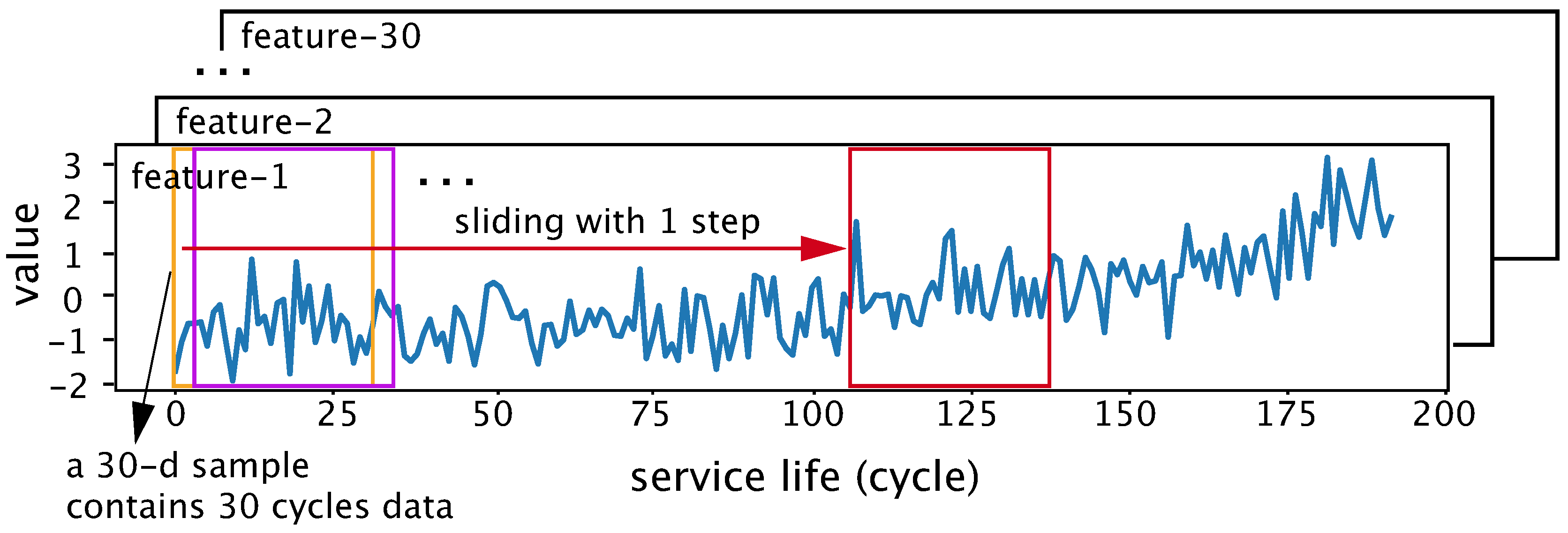
All training and test datasets are shown in Table 1. Single-cycle data in the C-MAPSS dataset is a 30-dimensional feature vector, consisting of 3 operational settings, 21 sensor values and 6 one-hot encoding values. Each input sample in our networks contains 30 single-cycle data which are extracted from every multivariate time series of trajectories as shown in Figure 3. The step size of the sliding window is 1. The true RUL of a sample is determined by the true RUL of the last single-cycle data. For training data, 40% of trajectories are randomly selected as validation data. For testing data, the last slide window of every trajectory is selected as the input data.
2.3.3. Evaluation
To evaluate the performance of our RUL estimation model on the test data, two measures are used here: Scoring Fuction and Root Mean Square Error (RMSE).
The scoring function proposed in PHM 2008 Data Challenge [37] is shown in Equation (10), where n is the total number of trajectories, , is estimated RUL and is the true RUL. This scoring function gives two different penalties. The penalty (estimated RUL is less than the true RUL) is smaller than the penalty (estimated RUL is larger than true RUL). The justification for this difference is that when , we still have time to conduct system maintenance; but when , the maintenance would be scheduled later than the required time, which may cause system failure.
RMSE is also widely used as an evaluation metric for RUL estimation, as shown in Equation (11). RMSE gives the same penalty weights for and for .
We used the mean score function as the loss function for training our networks, as shown below.
where S is calculated from Equation (10), n is the total number of trajectories.
2.4. Data Preprocessing
2.4.1. Data Normalization
There are several ways to normalize the sensor data. Here we used standardization to remove the mean and scale the data with unit variance. We standardize the data by Equation (13), where is the ith sensor data, is the normalized data, is the mean of ith sensor data, is the ith corresponding standard deviation.
2.4.2. Operating Conditions
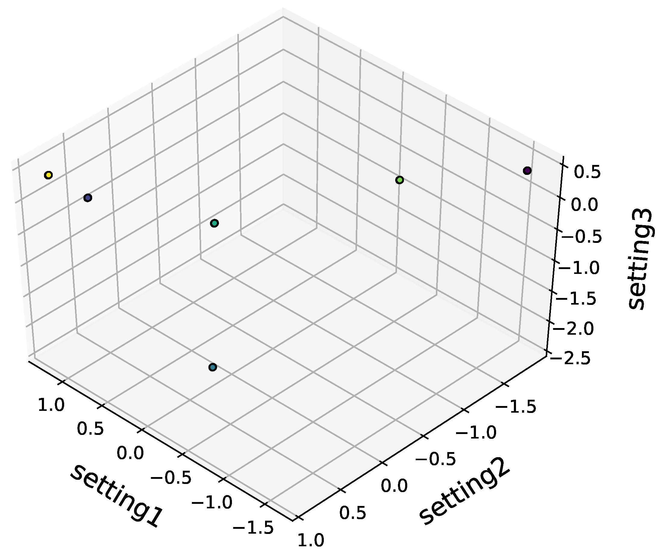
Previous research [23,24,37] on the C-MAPSS dataset showed that the operating setting in this dataset can be clustered into six distinct groups, each representing a distinct operating condition. Here we used the K-means algorithm to cluster operating setting values in all datasets into 6 clusters as shown in Figure 4. Based on clustering, an operating setting label can be represented as a 6-dimension vector using one-hot encoding.
2.4.3. RUL Target Function
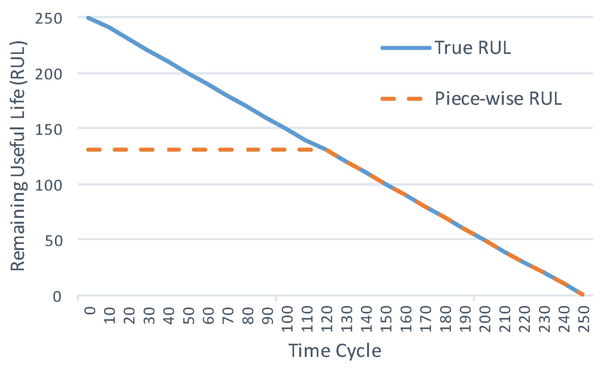
The traditional way to define the degradation process in a system is using a linear model along time. However, in practical applications, the degradation in a system is negligible at the beginning of use and increases after an anomaly point. It is hard to estimate RUL before the anomaly point. Besides, estimating RUL before the anomaly point during which the system works well is not useful in practical applications. Hence, for the C-MAPSS datasets, a piece-wise linear degradation model was proposed in [37], which limits the maximum value of the RUL function as illustrated in Figure 5.
In this paper, we set the maximum RUL limit as 130 time cycles, the same as in [37]. We ignore data whose true RULs are greater than the maximum limit to pay attention to the degradation data.
3. Experiments and Results
To verify the performance of our BLSTM-based transfer learning algorithm for RUL estimation, we conducted a series of experiments on the C-MAPSS Datasets. We evaluated the performance of transfer learning over every dataset and studied how different working conditions and the numbers of samples for each pair of source and target datasets affect the performance of the resulting prediction models.
We designed four groups of without-transfer learning experiments (E1, E4, E7, E10) and eight groups of transfer learning experiments (E2, E3, E5, E6, E8, E9, E11, E12) involving 4 groups of target datasets (FD001, FD002, FD003, FD004) as shown in Table 2. For each group of target datasets, we randomly selected 10, 20, ..., 90, 100 trajectories to generate 10 datasets from which 10 evaluation datasets are generated. This will allow us to evaluate how the number of samples in the target dataset affects the performance of transfer learning.
For each transfer experiment, we compared the performance of standard BLSTM models over the target dataset without transfer learning against the performance of the BLSTM models with transfer learning. We repeated each such experiment three times to deal with the randomness of the algorithms. In total, we have conducted 10 × 3 × (8 + 4) = 360 experiments, where 10 is the number evaluation datasets, each with different numbers of train trajectories; 3 is the number of repeats for each experiment; 8 is the number of transfer experiment pairs; 4 is the number of experiments without transfer. For all experiments, the performances of the experiment were evaluated by score function and RMSE. Note that the experiment group of E2 and E3 have the same target data but different source data, and compare with the experiment group of E1. The same is true for E5 and E6 groups who compare with E4 group, E8 and E9 groups who compare with E7 group, and E11 and E12 groups who compare with E10 group.
Table 3 shows the results of all experiments in terms of the mean values of the performance scores and RMSE. IMP is the improvement of the models with transfer learning over those without transfer learning. It is defined as . From the IMP values, we can easily observe that transfer learning made great improvement except for groups E3 and E9, which will be explained in Section 4 (E3 and E9 are multiple operating conditions to 1 condition). For example, when the number of trajectories used is less than or equal to 60, transfer learning has improved the performance scores from 16.41% to 85.12% for group E2. Similar improvements are also observed for groups E5, E6, E8, E11, and E12.
In particular, we found transfer learning is more effective in general on models trained with small data sets. For example, it improves the model score by 43.19% for group E5 when only 10 trajectories are used to create the training sets, while the improvement is only 8.29% when 60 trajectories are used as training sets for the same E5 group.
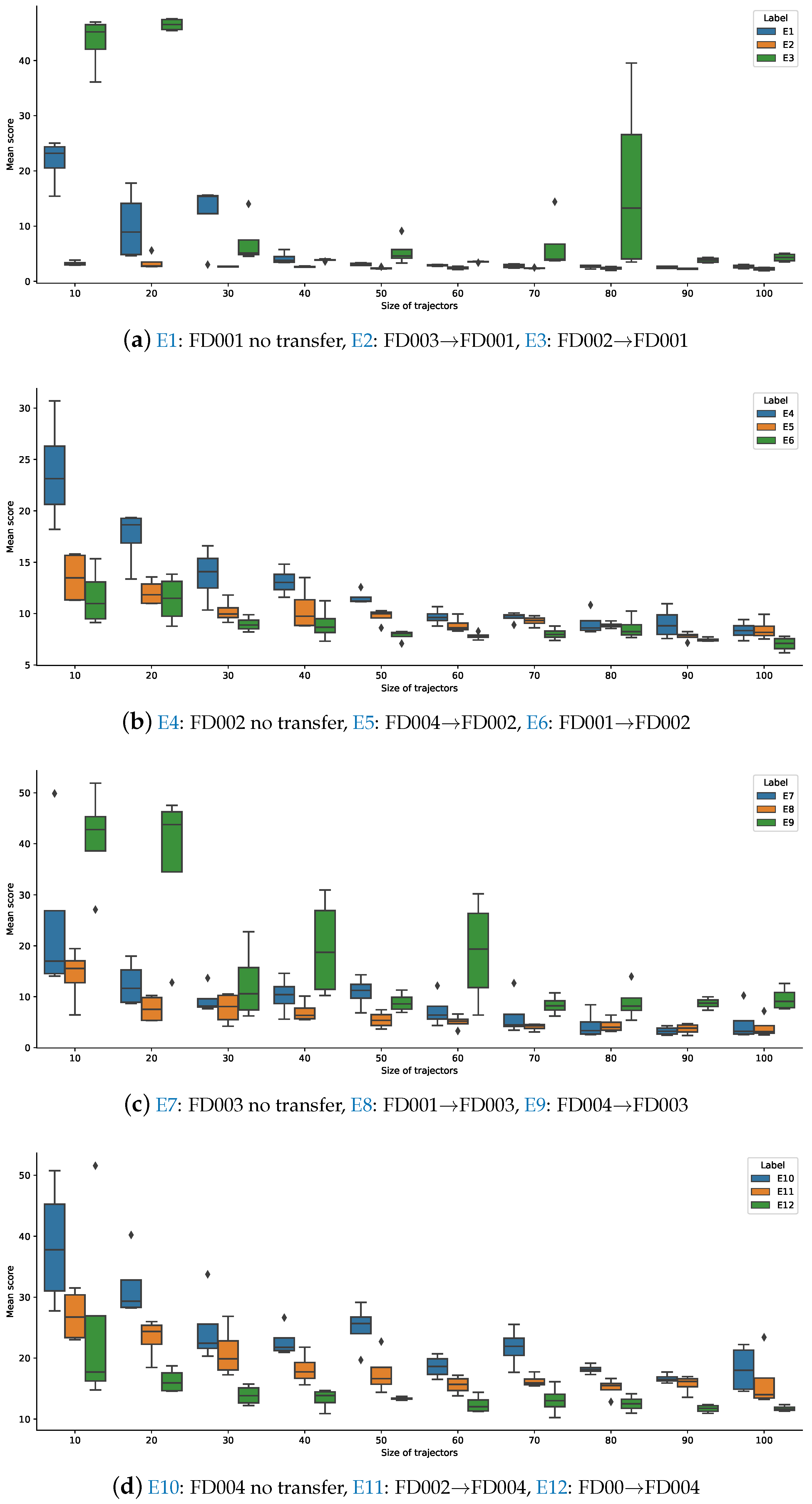
We also found that the changes of Mean Score and RMSE have similar trends. In Figure 6 we showed the box plot of the Mean Scores to illustrate the distribution of every transfer learning experiment. Figure 6a–d respectively illustrate the performance of four groups of dataset target models (FD001, FD002, FD003, and FD004). The blue boxes are the performance without transfer and the yellow and green boxes are the performance with transfer. In Figure 6a, the transfer experiment E2 is more stable and gets lower mean score than the without-transfer experiment E1. In Figure 6b, both the transfer experiment E5 and E6 are more stable and get lower mean score than the without-transfer experiment E4. In Figure 6c, the transfer experiment E8 is more stable and gets a lower mean score than the without-transfer experiment E7. In Figure 6d, both the transfer experiment E11 and E12 are more stable and get lower mean score than the without-transfer experiment E10. Thus, from the distribution of box plots for experiments, we can easily observe that the performance of models with transfer learning are more stable and make great improvement than those without transfer learning except the transfer experiment E3 and E9, which will be explained in Section 4.
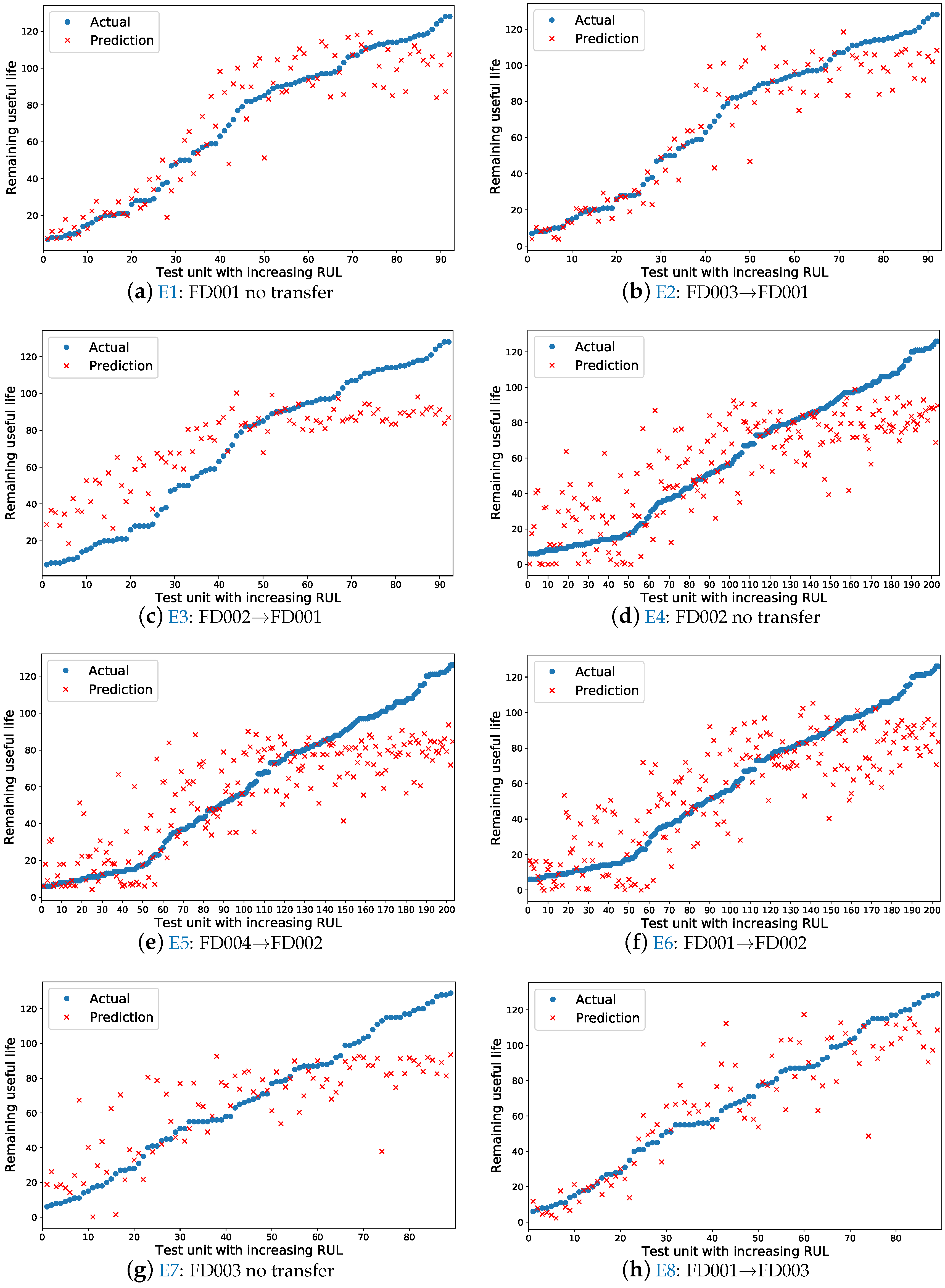
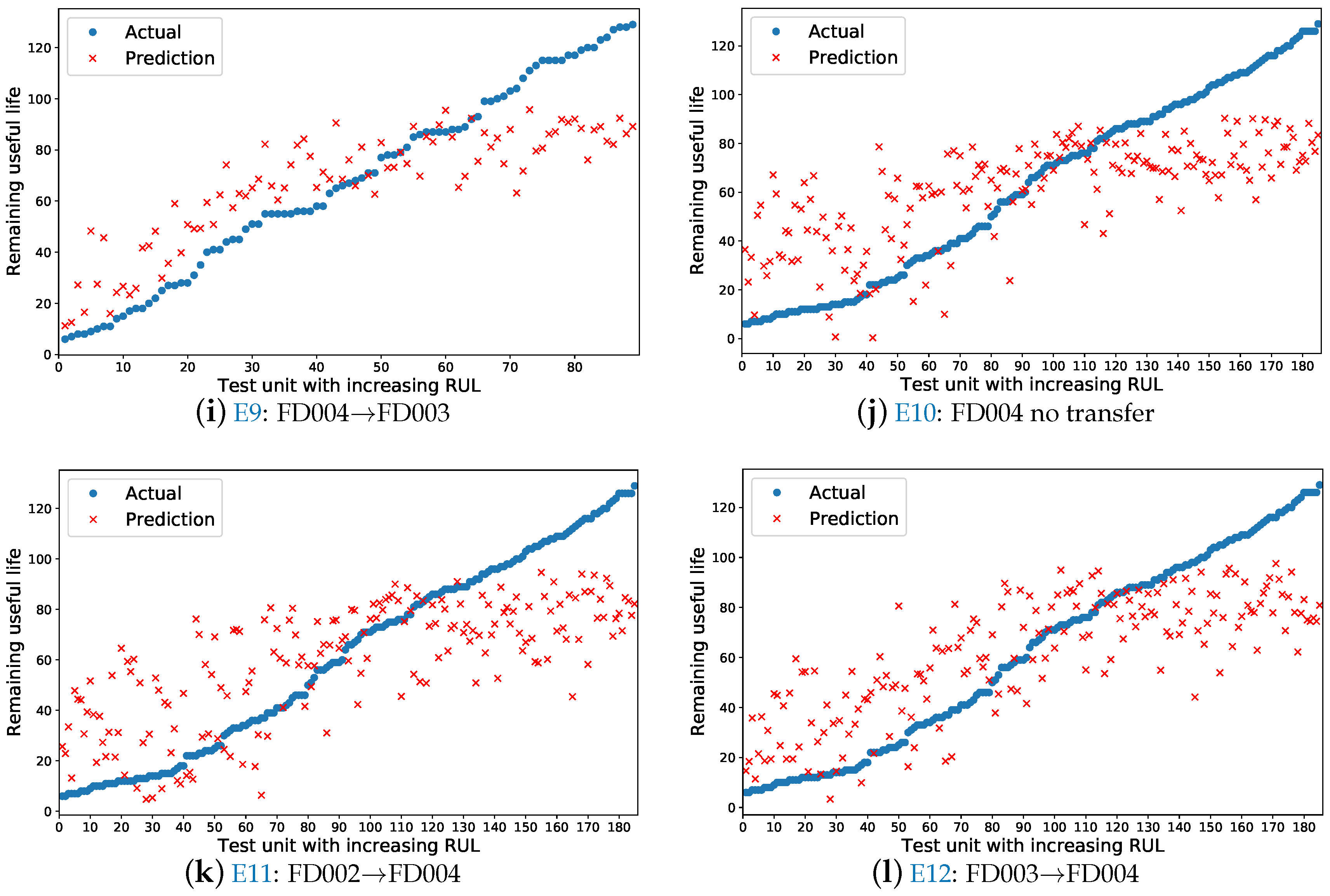
Figure 7 illustrates the RUL estimation results in test data for experiments, in which the training data set is generated by randomly selected 50 trajectories. Those figures show and compare the RUL estimation results for four test data sets (FD001, FD002, FD003, FD004). Figure 7a,d,j are the without-transfer experiment and others are the transfer experiments. For every figure, the X-axis is the test unit with increasing RUL, which is sorted by actual RUL values. The Y-axis is the actual and prediction RUL value. The blue points are the actual RUL value of test unit and the red points are the prediction RUL value of test unit. Comparing with Figure 7a,b, we found that the prediction RUL values in the transfer experiment E2 (Figure 7b) are nearer to the actual RUL values than in the without-transfer experiment E1 (Figure 7a). Comparing with Figure 7d–f, we found that both the prediction RUL values in the transfer experiment E5 (Figure 7e) and E6 (Figure 7f) are nearer to the actual RUL values than in the without-transfer experiment E4 (Figure 7d). Comparing with Figure 7g,h, we found that the prediction RUL values in the transfer experiment E8 (Figure 7h) are nearer to the actual RUL values than in the without-transfer experiment E7 (Figure 7g). Comparing with Figure 7j–l, we found that both the prediction RUL values in the transfer experiment E11 (Figure 7k) and E12 (Figure 7l) are nearer to the actual RUL values than in the without-transfer experiment E10 (Figure 7j). For these figures, comparing between transfer and no-transfer learning performance, we found that the effect of transfer experiments performance is obvious except for E3 and E9, which will be explained in Section 4.
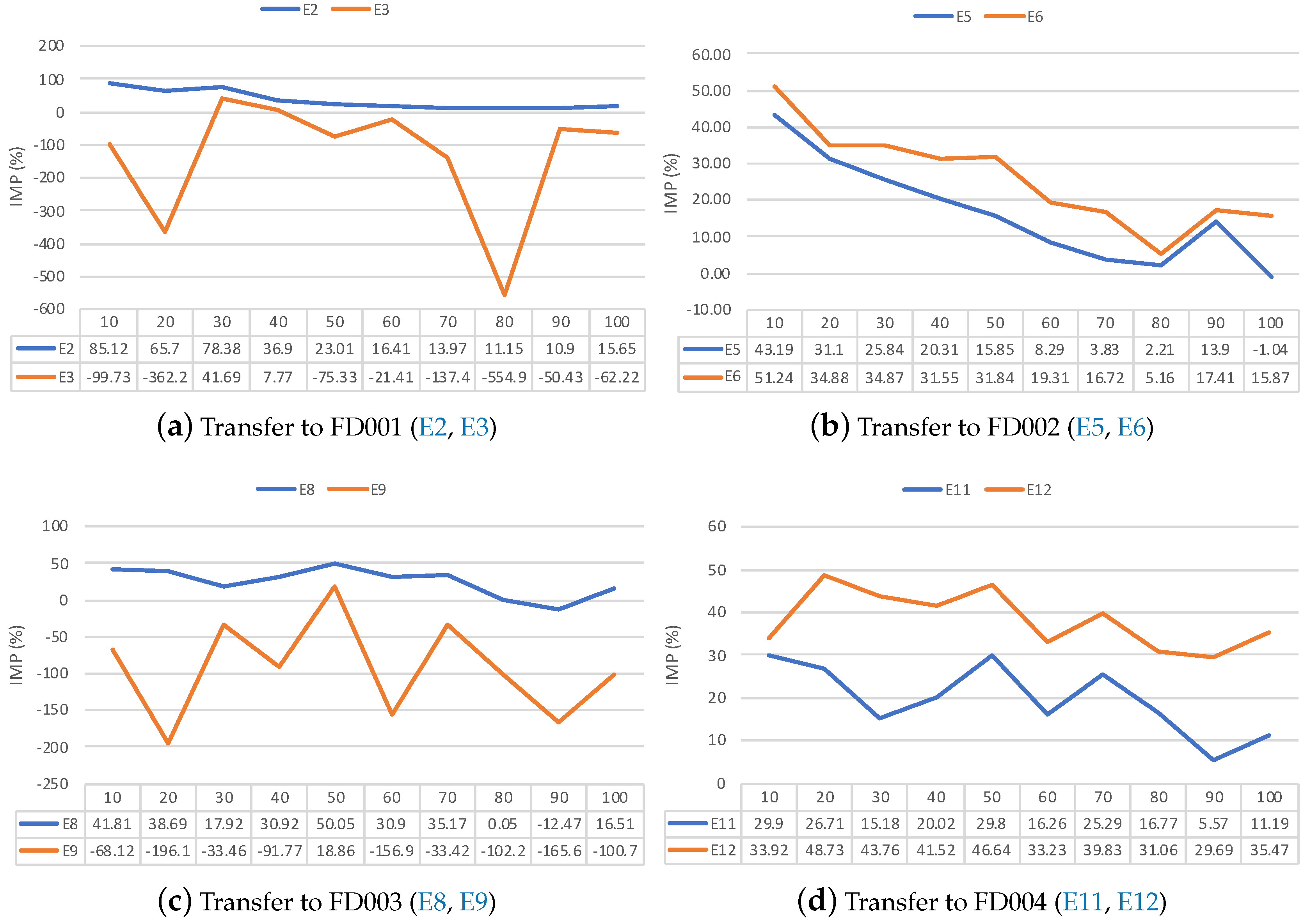
To further examine how different transfer learnings work, we analyzed the IMP performances of a transfer experiment which transfers from different source datasets to the same target datasets. In Figure 8, Figure 8a–d respectively illustrate the improvement performance of transferring to four datasets (FD001, FD002, FD003, and FD004). Figure 8a shows the IMP performance of transfer experiment which transfers to FD001 target dataset. The E2 has effective performance. The IMP performance in the E2 is greater than 20% when the size of trajectories is less than or equal than 50. The E3 has a detrimental effect performance. Figure 8b shows the IMP performance of a transfer experiment which transfers to the FD002 target dataset. Both the E5 and E6 have effective performance. The IMP performance in the E5 is greater than 15% when the size of trajectories is less than or equal than 50. The IMP performance in the E6 is greater than 45% when the size of trajectories less than or equal than 50. Figure 8c shows the IMP performance of a transfer experiment which transfers to the FD0013 target dataset. The E8 has effective performance. The IMP performance in the E8 is greater than 17% when the size of trajectories is less than or equal than 70. The E9 has a detrimental effect on performance. Figure 8d shows the IMP performance of a transfer experiment which transfers to the FD004 target dataset. Both the E5 and E6 have effective performance. The IMP performance in the E5 is greater than 15% when the size of trajectories is less than or equal than 50. The IMP performance in the E6 is greater than 30% when the size of the trajectories is less than or equal than 50.
From all the above results, we also found that working conditions affect transfer learning performance a lot. How do working conditions affect transfer learning performance? We will discuss this in Section 4.
4. Discussion
In the prior section, we showed that transfer learning is effective, except for E3 and E9. Here, we discuss how working conditions affect the transfer performance and analyze the cases when transfer learning can bring negative effects.
4.1. How Working Conditions Affect Transfer Learning Performance
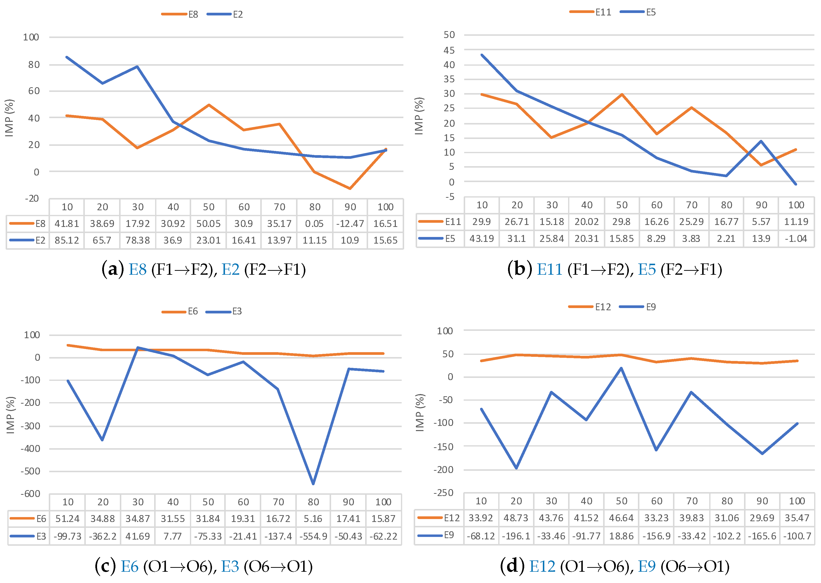
To further understand how working conditions affect transfer learning performance, we analyzed the IMP performances of transfer experiments grouped by different working conditions. Figure 9 shows the IMP performance of transfer learning with different working conditions. Table 4 shows the information of experiments in Figure 9. Figure 9a,b show how fault conditions influence the performance of transfer learning. Figure 9c,d show how operating conditions influence the performance of transfer learning.
From Figure 9a,b, we found that when the fault conditions are considered, in both the transfer learning from single fault condition to multiple fault conditions (E8, E11) and the transfer learning from multiple fault conditions to single fault condition (E2, E5), the transfer learning scheme improved the prediction models of the target dataset.
From Figure 9c,d, we found that when the operating conditions are considered, transfer learning from a single operating condition to multiple operating conditions (E6, E12) improved the prediction performance of the model on target dataset. However, transfer learning from the model trained on the multiple operating condition dataset to the single operating condition (E3, E9) had a detrimental effect on the prediction performance of the target model.
From all the above results, we found that transfer learning under working conditions made effective performance improvements, except when transferring from multiple operating conditions to single operating condition (E3, E9).
4.2. Negative Transfer
Negative transfer occurs when the information learned from the source domain has a detrimental effect on the prediction model for the target domain [29]. The more the source data is similar to the target data, the lower the negative transfer effect. We already noted that transfer from multiple operating conditions to single condition led to a detrimental effect. Here we try to understand the negative transfer by comparing sensors’ monitoring data values and explain why transfer from multiple operating conditions to a single condition has a detrimental effect.
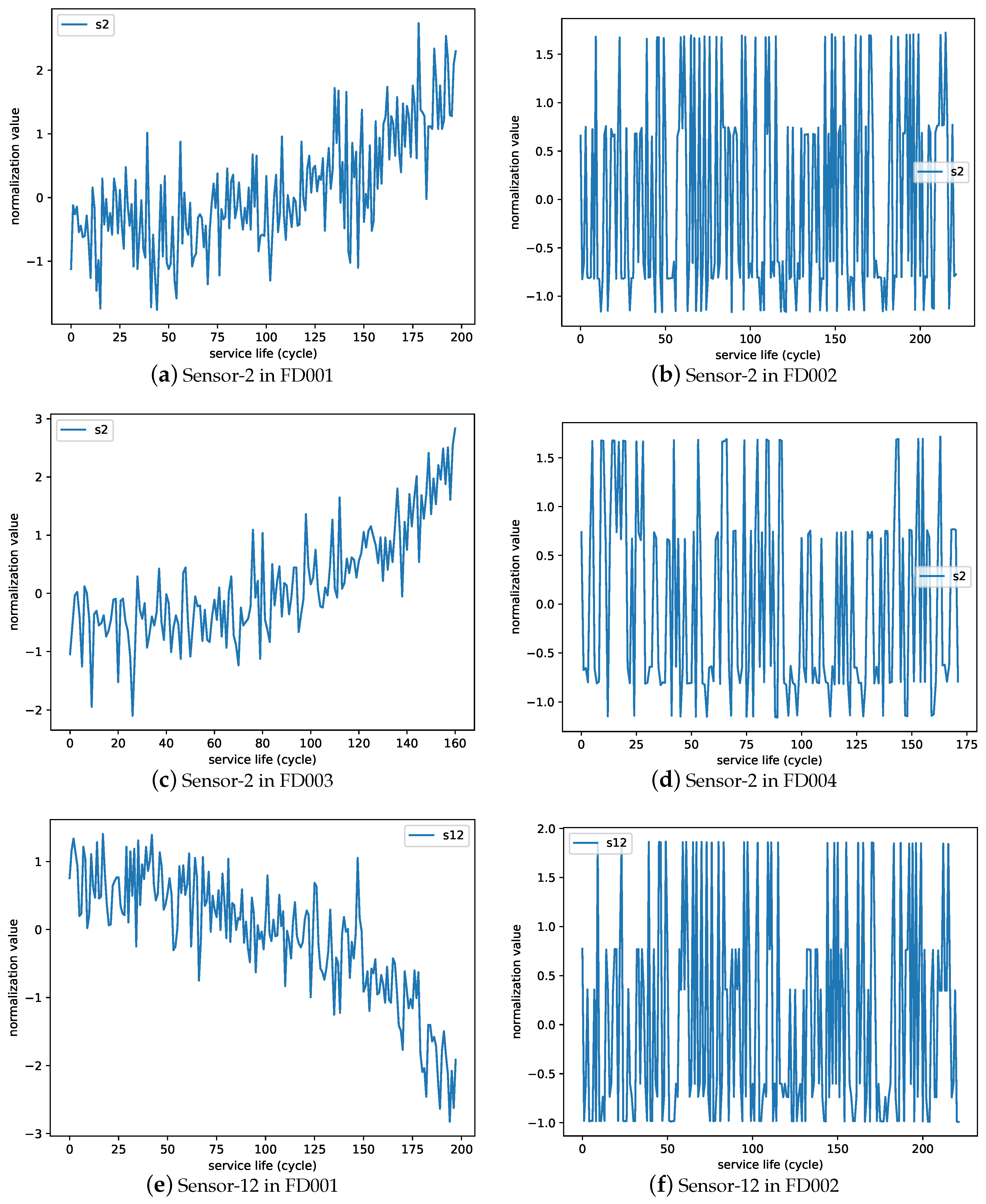
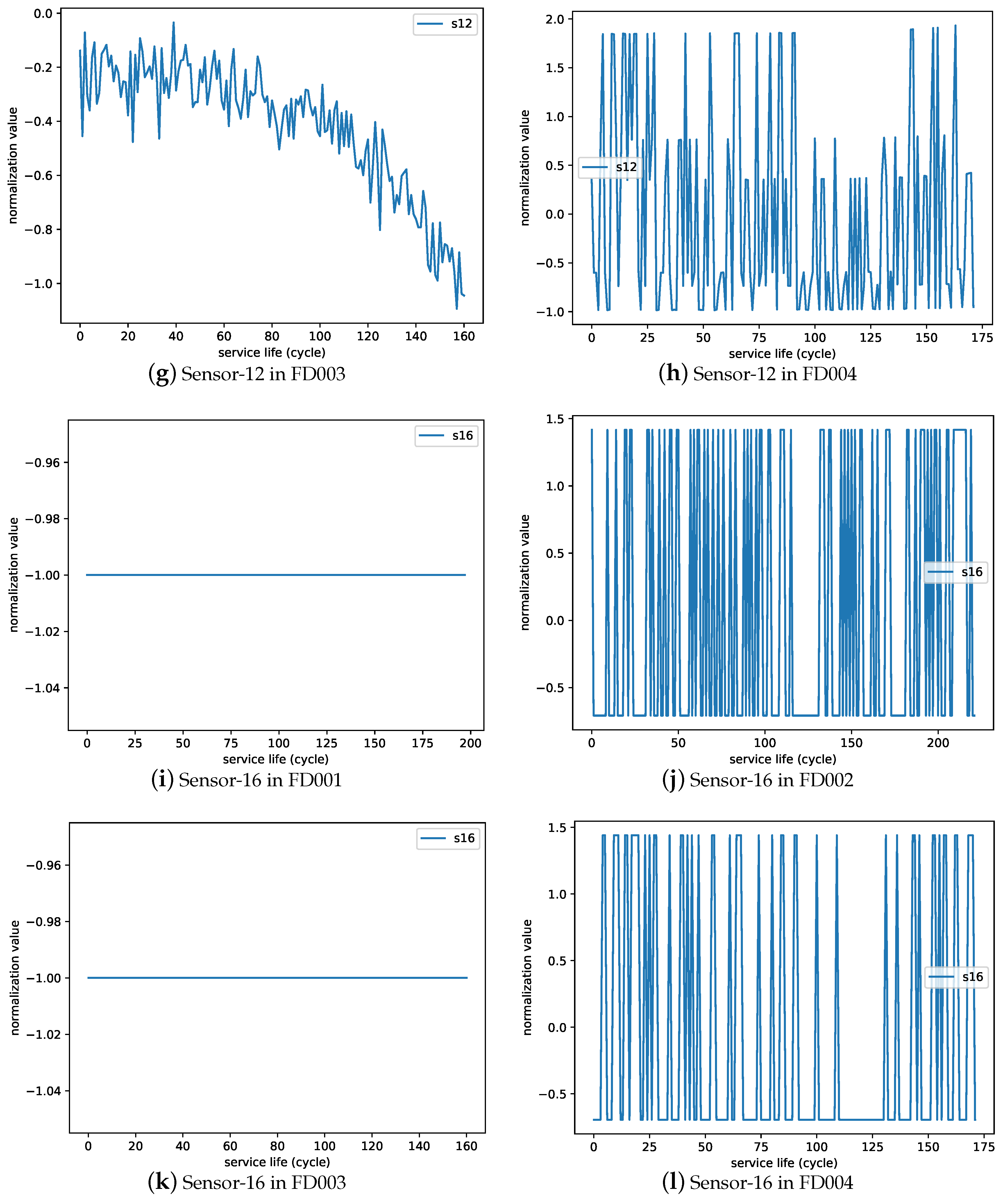
Figure 10 shows the comparison between three type trends of sensors’ monitoring data values in each of the following datasets (FD001, FD002, FD003, FD004). Figure 10a–d are the sensor-2 values, which represent the ascending trend sensors. Figure 10e–h are the sensor-12 values, which represent the descending trend sensors. Figure 10i–l are the sensor-16 values, which represent the trend that is unchanged in FD001 and FD003 but changed in FD002 and FD004. It is important to note that the operating setting values have great influence on sensor values and influence transfer learning performance a lot.
Comparing Figure 10a,e,i with Figure 10c,g,k, FD001 and FD003 have different fault conditions. We found that the distribution of sensor values with different fault condition are similar. The same is true for FD002 in Figure 10b,f,j and FD004 in Figure 10d,h,l. Since the distribution of sensor values with different fault conditions are similar, the transfer learning from single to the multiple fault conditions (E8, E11) and from multiple to single fault conditions (E2, E5) can achieve positive effects on the prediction model of the target dataset.
Comparing Figure 10a,e,i with Figure 10b,f,j, FD001 and FD002 have different operating conditions. We found that the distribution of sensor values with different operating conditions have large differences. The same is true for FD003 in Figure 10c,g,k and FD004 Figure 10d,h,l. With the understanding that the distribution of sensor values with different operating conditions have big differences, our experiments showed that the transfer learning from multiple to single operating conditions (E3, E9) led to a detrimental effect on prediction performance while transfer learning from single to multiple operating conditions (E6, E12) led to a positive effect on the prediction performance of the target model.
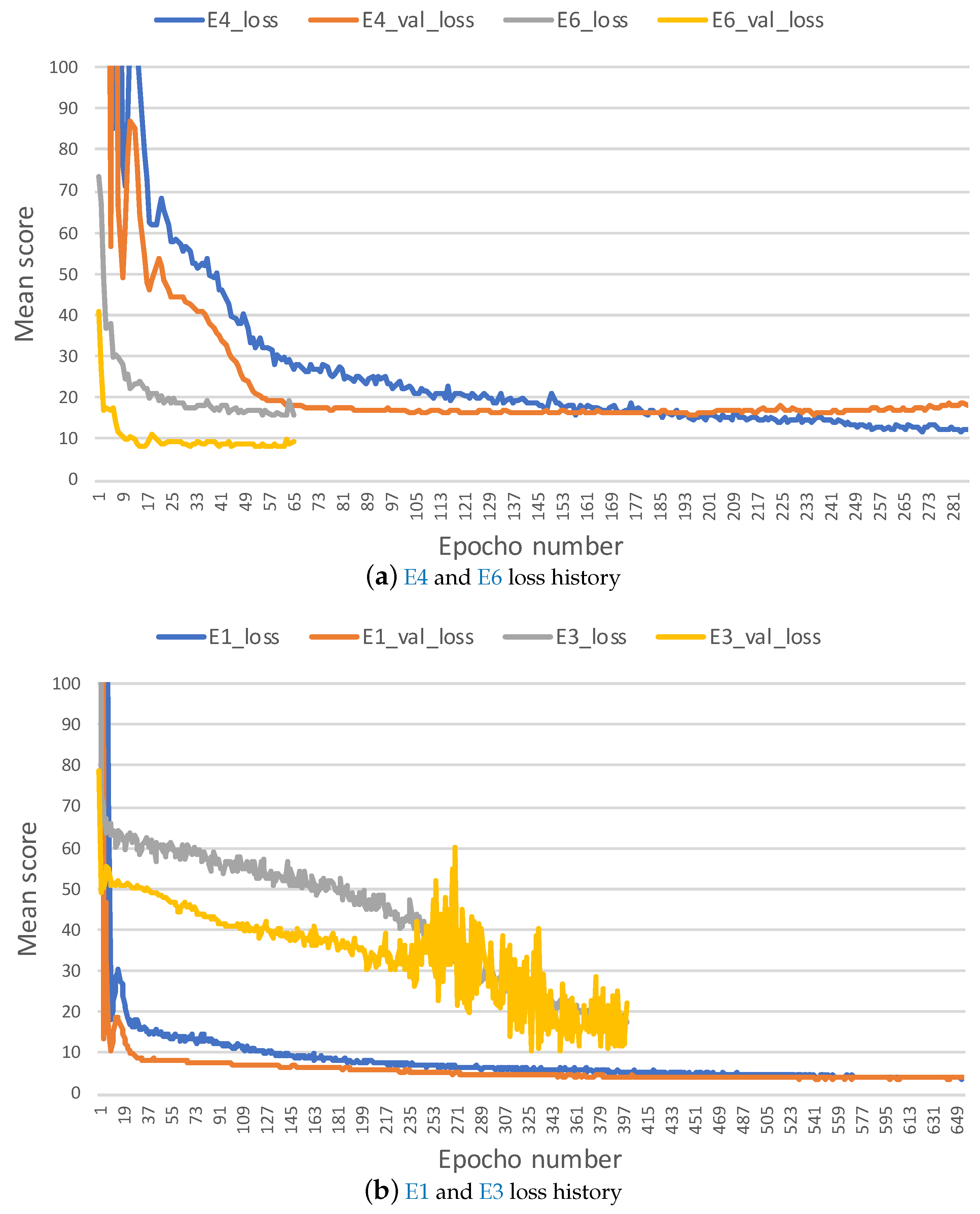
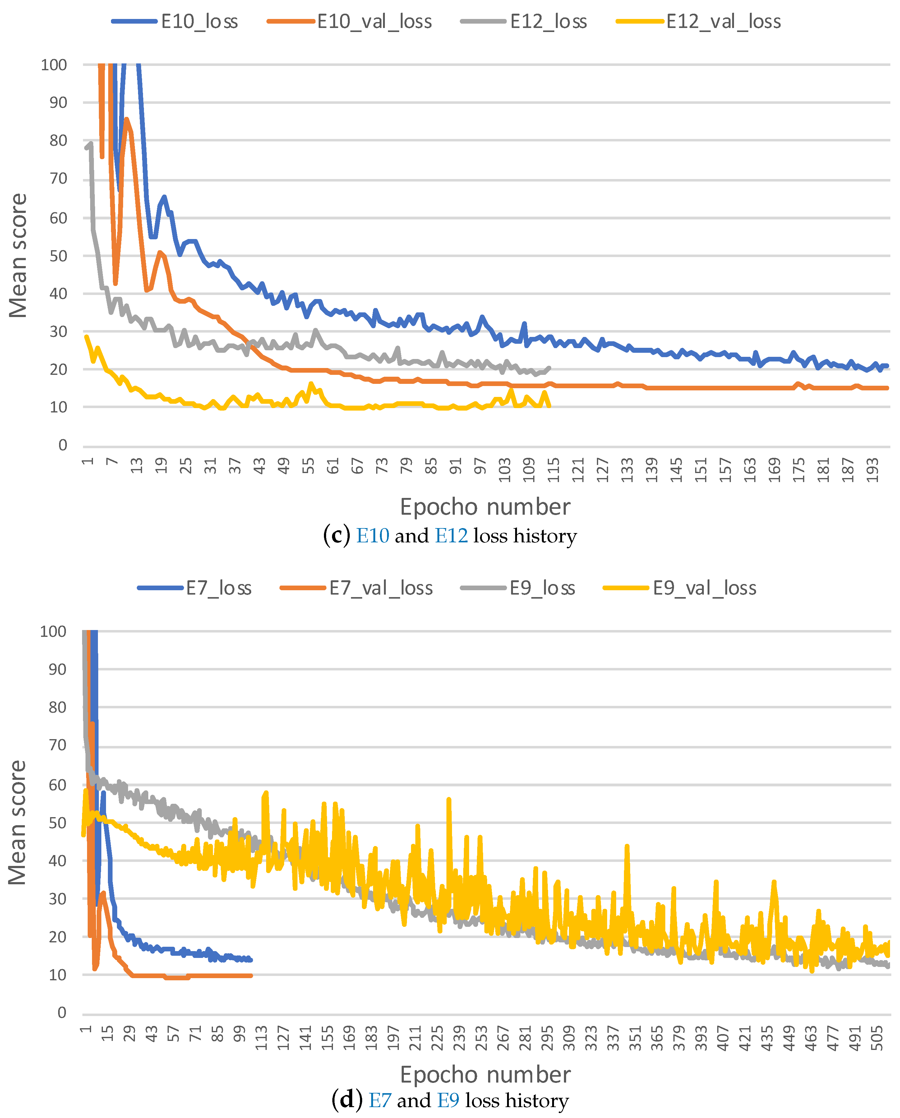
What causes the different effects of transfer learning with different operating conditions? Two factors may be involved here. First, we found that the sensor monitoring data under the multiple operating conditions are more complicated than the dataset under single conditions. Second, the distribution of sensor values are more different than the sensor monitoring data with the single operating condition. And then the initial parameters of the model transferred from the complicated multiple conditions to the simple single condition causes overfitting and it is hard to fine-tune it with limited target data size. This can be verified from the plots of training loss history. Figure 11 illustrates the training loss history for experiments in which the training data set is generated by randomly selecting 50 trajectories. Comparing training loss history between Figure 11a and Figure 11b, we found that E6 in Figure 11a is able to fine-tune training well and gets a lower mean score by nearly 10 in validation data than experiments without transfer E4 in Figure 11a. However, E3 causes overfitting. It is hard to fine-tune training and it gets a higher mean score by nearly 20 on validation data than experiments without transfer E1. The same is true between E12 in Figure 11c and E9 in Figure 11d. This may explain why transfer learning from multiple operating conditions to a single condition led to detrimental effects on the prediction performance.
5. Conclusions
This paper presents a transfer learning algorithm with bi-directional LSTM neural networks for RUL prediction of a turbofan engine. Our algorithm addresses one of the major challenges in RUL prediction: the difficulty of obtaining a sufficient number of samples in data-driven prognostics. Our transfer prognostic model works by exploiting data samples from different but approximately related tasks for remaining useful life estimation. Our method was validated on the C-MAPSS Datasets with extensive experiments by comparing its performance with those models without transfer learning. The experimental results showed that transfer learning is effective in most cases except when transferring from a dataset of multiple operating conditions to a dataset of a single operating condition, which led to negative transfer learning. How to prevent negative transfer is still an open problem. In future work, we will develop more advanced transfer learning methods or data normalization schemes to improve the multi-condition RUL prediction performance.
Author Contributions
Conceptualization, A.Z., J.H., S.L.; methodology, A.Z., J.H., Z.L., Y.C.; software, A.Z., G.Y.; investigation, A.Z., J.H.; resources, S.L.; writing—original draft preparation, A.Z., J.H.; writing—review and editing, A.Z., J.H., Z.L. and Y.C.; supervision, S.L. and J.H.; project administration, H.W., J.H. and S.L.; funding acquisition, H.W. and S.L.
Funding
This research was funded by The National Natural Science Foundation of China under Grant Nos. 91746116 and 51741101, Project of Ministry of Industry and Information under Grant No. [2016]213, Science and Technology Project of Guizhou Province under Grant Nos. Talents [2015]4011 and [2016]5013, Collaborative Innovation [2015]02, National Natural Science Foundation of China: 61863005 and Project of Guizhou University’s Technology Crowdfunding for Intelligent Equipment under Grant No. JSZC[2016]001.
Acknowledgments
J.H. gratefully acknowledge the support of NVIDIA Corporation with the donation of the Titan X Pascal GPU used for this research and the support of National Institute of Measurement and Testing Technology with providing the semi-anechoic laboratory.
Conflicts of Interest
The authors declare no conflict of interest.
References
- Lei, Y.; Li, N.; Guo, L.; Li, N.; Yan, T.; Lin, J. Machinery health prognostics: A systematic review from data acquisition to RUL prediction. Mech. Syst. Signal Process. 2018, 104, 799–834. [Google Scholar] [CrossRef]
- Lu, C.; Wang, Z.Y.; Qin, W.L.; Ma, J. Fault diagnosis of rotary machinery components using a stacked denoising autoencoder-based health state identification. Signal Process. 2017, 130, 377–388. [Google Scholar] [CrossRef]
- Zhu, S.P.; Huang, H.Z.; Peng, W.; Wang, H.K.; Mahadevan, S. Probabilistic physics of failure-based framework for fatigue life prediction of aircraft gas turbine discs under uncertainty. Reliab. Eng. Syst. Saf. 2016, 146, 1–12. [Google Scholar] [CrossRef]
- Yin, S.; Li, X.; Gao, H.; Kaynak, O. Data-based techniques focused on modern industry: An overview. IEEE Trans. Ind. Electron. 2015, 62, 657–667. [Google Scholar] [CrossRef]
- Lee, J.; Wu, F.; Zhao, W.; Ghaffari, M.; Liao, L.; Siegel, D. Prognostics and health management design for rotary machinery systems—Reviews, methodology and applications. Mech. Syst. Signal Process. 2014, 42, 314–334. [Google Scholar] [CrossRef]
- Lu, J.; Lu, F.; Huang, J. Performance Estimation and Fault Diagnosis Based on Levenberg–Marquardt Algorithm for a Turbofan Engine. Energies 2018, 11, 181. [Google Scholar] [Green Version]
- Fumeo, E.; Oneto, L.; Anguita, D. Condition based maintenance in railway transportation systems based on big data streaming analysis. Procedia Comput. Sci. 2015, 53, 437–446. [Google Scholar] [CrossRef]
- Stetter, R.; Witczak, M. Degradation Modelling for Health Monitoring Systems. In Journal of Physics: Conference Series; IOP Publishing: Bristol, UK, 2014; Volume 570, p. 062002. [Google Scholar]
- Khelassi, A.; Theilliol, D.; Weber, P.; Ponsart, J.C. Fault-tolerant control design with respect to actuator health degradation: An LMI approach. In Proceedings of the 2011 IEEE International Conference on Control Applications (CCA), Denver, CO, USA, 28–30 September 2011; pp. 983–988. [Google Scholar]
- Jardine, A.K.; Lin, D.; Banjevic, D. A review on machinery diagnostics and prognostics implementing condition-based maintenance. Mech. Syst. Signal Process. 2006, 20, 1483–1510. [Google Scholar] [CrossRef]
- Eker, O.F.; Camci, F.; Jennions, I.K. Major Challenges in Prognostics: Study on Benchmarking Prognostics Datasets. In Proceedings of the First European Conference of the Prognostics and Health Management Society 2012, Dresden, German, 3–5 July 2012. [Google Scholar]
- Liu, K.; Chehade, A.; Song, C. Optimize the signal quality of the composite health index via data fusion for degradation modeling and prognostic analysis. IEEE Trans. Autom. Sci. Eng. 2017, 14, 1504–1514. [Google Scholar] [CrossRef]
- Lei, Y.; Li, N.; Gontarz, S.; Lin, J.; Radkowski, S.; Dybala, J. A model-based method for remaining useful life prediction of machinery. IEEE Trans. Reliab. 2016, 65, 1314–1326. [Google Scholar] [CrossRef]
- Camci, F.; Medjaher, K.; Zerhouni, N.; Nectoux, P. Feature evaluation for effective bearing prognostics. Qual. Reliab. Eng. Int. 2013, 29, 477–486. [Google Scholar] [CrossRef] [Green Version]
- Camci, F.; Chinnam, R.B. Health-state estimation and prognostics in machining processes. IEEE Trans. Autom. Sci. Eng. 2010, 7, 581–597. [Google Scholar] [CrossRef] [Green Version]
- Diamanti, K.; Soutis, C. Structural health monitoring techniques for aircraft composite structures. Prog. Aerosp. Sci. 2010, 46, 342–352. [Google Scholar] [CrossRef]
- Gebraeel, N.; Elwany, A.; Pan, J. Residual life predictions in the absence of prior degradation knowledge. IEEE Trans. Reliab. 2009, 58, 106–117. [Google Scholar] [CrossRef]
- Eker, O.F.; Camci, F.; Guclu, A.; Yilboga, H.; Sevkli, M.; Baskan, S. A simple state-based prognostic model for railway turnout systems. IEEE Trans. Ind. Electron. 2011, 58, 1718–1726. [Google Scholar] [CrossRef] [Green Version]
- LeCun, Y.; Bengio, Y.; Hinton, G. Deep learning. Nature 2015, 521, 436. [Google Scholar] [CrossRef] [PubMed]
- Li, S.; Liu, G.; Tang, X.; Lu, J.; Hu, J. An ensemble deep convolutional neural network model with improved ds evidence fusion for bearing fault diagnosis. Sensors 2017, 17, 1729. [Google Scholar] [CrossRef] [PubMed]
- Li, S.; Yao, Y.; Hu, J.; Liu, G.; Yao, X.; Hu, J. An ensemble stacked convolutional neural network model for environmental event sound recognition. Appl. Sci. 2018, 8, 1152. [Google Scholar] [CrossRef]
- Yao, Y.; Wang, H.; Li, S.; Liu, Z.; Gui, G.; Dan, Y.; Hu, J. End-to-end convolutional neural network model for gear fault diagnosis based on sound signals. Appl. Sci. 2018, 8, 1584. [Google Scholar] [CrossRef]
- Babu, G.S.; Zhao, P.; Li, X.L. Deep Convolutional Neural Network Based Regression Approach for Estimation of Remaining Useful Life. In International Conference on Database Systems for Advanced Applications; Springer: Cham, Switzerland, 2016; pp. 214–228. [Google Scholar]
- Zheng, S.; Ristovski, K.; Farahat, A.; Gupta, C. Long short-term memory network for remaining useful life estimation. In Proceedings of the 2017 IEEE International Conference on IEEE Prognostics and Health Management (ICPHM), Allen, TX, USA, 19–21 June 2017; pp. 88–95. [Google Scholar]
- Zhao, R.; Yan, R.; Wang, J.; Mao, K. Learning to monitor machine health with convolutional Bi-directional LSTM networks. Sensors (Switzerland) 2017, 17, 273. [Google Scholar] [CrossRef] [PubMed]
- Wu, Y.; Yuan, M.; Dong, S.; Lin, L.; Liu, Y. Remaining useful life estimation of engineered systems using vanilla LSTM neural networks. Neurocomputing 2018, 275, 167–179. [Google Scholar] [CrossRef]
- Li, Z.; Wu, D.; Hu, C.; Terpenny, J. An ensemble learning-based prognostic approach with degradation-dependent weights for remaining useful life prediction. Reliab. Eng. Syst. Saf. 2018. [Google Scholar] [CrossRef]
- Pan, S.J.; Yang, Q. A survey on transfer learning. IEEE Trans. Knowl. Data Eng. 2010, 22, 1345–1359. [Google Scholar] [CrossRef]
- Weiss, K.; Khoshgoftaar, T.M.; Wang, D.D. A Survey of Transfer Learning. J. Big Data 2016. [Google Scholar] [CrossRef]
- Meng, Z.; Chen, Z.; Mazalov, V.; Li, J.; Gong, Y. Unsupervised adaptation with domain separation networks for robust speech recognition. In Proceedings of the 2017 IEEE Automatic Speech Recognition and Understanding Workshop (ASRU), Okinawa, Japan, 16–20 December 2017; pp. 214–221. [Google Scholar]
- Singh, K.K.; Divvala, S.; Farhadi, A.; Lee, Y.J. DOCK: Detecting Objects by Transferring Common-Sense Knowledge. In European Conference on Computer Vision; Springer: Berlin, Germany, 2018; pp. 506–522. [Google Scholar]
- Cao, H.; Bernard, S.; Heutte, L.; Sabourin, R. Improve the performance of transfer learning without fine-tuning using dissimilarity-based multi-view learning for breast cancer histology images. In International Conference Image Analysis and Recognition; Springer: Berlin, Germany, 2018; pp. 779–787. [Google Scholar]
- Ramasso, E.; Saxena, A. Performance Benchmarking and Analysis of Prognostic Methods for CMAPSS Datasets. Int. J. Prognostics Health Manag. 2014, 5, 1–15. [Google Scholar]
- Saxena, A.; Goebel, K. Turbofan Engine Degradation Simulation Data Set. NASA Ames Prognostics Data Repository. 2008. Available online: https://ti.arc.nasa.gov/tech/dash/groups/pcoe/prognostic-data-repository/ (accessed on 20 November 2018).
- Hochreiter, S.; Urgen Schmidhuber, J. LONG SHORT-TERM MEMORY. Neural Comput. 1997, 9, 1735–1780. [Google Scholar] [CrossRef] [PubMed]
- Graves, A.; Schmidhuber, J. Framewise phoneme classification with bidirectional LSTM and other neural network architectures. Neural Netw. 2005, 18, 602–610. [Google Scholar] [CrossRef] [PubMed] [Green Version]
- Heimes, F. Recurrent Neural Networks for Remaining Useful Life Estimation. In Proceedings of the International Conference on 2008 Prognostics and Health Management, Denver, CO, USA, 6–9 October 2008; pp. 1–6. [Google Scholar] [CrossRef]
Figure 1.
Operational setting values in every sub-dataset.

Figure 2.
Transfer learning model architecture.

Figure 3.
Extracting input samples.

Figure 4.
Operating setting clusters.

Figure 5.
Piece-wise linear RUL target function.

Figure 6.
Box plot of the mean score for every experiment. The blue boxes are the without-transfer model and the yellow and green boxes are the performance of transfer model. The X-axis is the size of trajectories which are randomly selected 10, 20, ..., 90, 100 trajectories. In the caption, A→B means from the source data A transfer to the target data B.

Figure 7.
Comparison of the RUL estimation results in test data for experiments of which the training data set is generated by randomly selecting 50 trajectories. In the subfigure, the X-axis is the test unit with increasing RUL which is sorted by actual RUL values. The Y-axis is the actual and prediction RUL values. The blue points are the actual RUL values of the test unit and the red points are the prediction RUL values of the test unit. In the subfigure caption, A→B means from the source data A transfer to the target data B.


Figure 8.
Comparison of the IMP performances for transfer experiments.

Figure 9.
Comparison of transfer learning performance improvement with different working conditions. In the caption, the F symbol is the fault condition, the O symbol is the operating condition, the number after the symbol is the type of working condition from the Table 2, and A→B means from working condition A transfer to working condition B.

Figure 10.
Comparison sensor monitoring data values.


Figure 11.
Training loss history for experiments in which the training data set is generated by randomly selecting 50 trajectories.
Figure 11.
Training loss history for experiments in which the training data set is generated by randomly selecting 50 trajectories.


Table 1.
C-MAPSS Datasets.
| Dataset | FD001 | FD002 | FD003 | FD004 |
|---|---|---|---|---|
| Dataset | FD001 | FD002 | FD003 | FD004 |
| Train trajectories | 100 | 260 | 100 | 249 |
| Test trajectories | 100 | 259 | 100 | 248 |
| Maximum life span (Cycles) | 362 | 378 | 525 | 543 |
| Average life span (Cycles) | 206 | 206 | 247 | 245 |
| Minimum life span (Cycles) | 128 | 128 | 145 | 128 |
| Operating Conditions | 1 | 6 | 1 | 6 |
| Fault conditions | 1 | 1 | 2 | 2 |
Table 2.
Experiments.
| Label | Transfer (From To) | Operating Conditions | Fault Conditions |
|---|---|---|---|
| E1 | FD001 no transfer | 1 | 1 |
| E2 | FD003→FD001 | 1→1 | 2→1 |
| E3 | FD002→FD001 | 6→1 | 1→1 |
| E4 | FD002 no transfer | 6 | 1 |
| E5 | FD004→FD002 | 6→6 | 2→1 |
| E6 | FD001→FD002 | 1→6 | 1→1 |
| E7 | FD003 no transfer | 1 | 2 |
| E8 | FD001→FD003 | 1→1 | 1→2 |
| E9 | FD004→FD003 | 6→1 | 2→2 |
| E10 | FD004 no transfer | 6 | 2 |
| E11 | FD002→FD004 | 6→6 | 1→2 |
| E12 | FD003→FD004 | 1→6 | 2→2 |
Table 3.
Experiments results in the mean values of very experiment that repeat three times.
| Label | From To/IMP | Mean Score | RMSE | ||||||||||||||||||
|---|---|---|---|---|---|---|---|---|---|---|---|---|---|---|---|---|---|---|---|---|---|
| 10 | 20 | 30 | 40 | 50 | 60 | 70 | 80 | 90 | 100 | 10 | 20 | 30 | 40 | 50 | 60 | 70 | 80 | 90 | 100 | ||
| E1 | FD001 no transfer | 21.71 | 10.06 | 12.35 | 4.17 | 3.07 | 2.9 | 2.76 | 2.65 | 2.54 | 2.65 | 26.36 | 22.07 | 21.18 | 16.62 | 15.12 | 15.06 | 14.64 | 14.62 | 14.2 | 14.26 |
| E2 | FD003→FD001 | 3.23 | 3.45 | 2.67 | 2.63 | 2.37 | 2.42 | 2.37 | 2.36 | 2.26 | 2.24 | 15.79 | 16.17 | 14.4 | 14.61 | 13.69 | 14.02 | 14.11 | 14.08 | 13.73 | 13.65 |
| IMP (%) | 85.12 | 65.7 | 78.38 | 36.9 | 23.01 | 16.41 | 13.97 | 11.15 | 10.9 | 15.65 | 40.09 | 26.7 | 31.99 | 12.12 | 9.41 | 6.88 | 3.63 | 3.66 | 3.31 | 4.22 | |
| E3 | FD002→FD001 | 43.36 | 46.51 | 7.2 | 3.84 | 5.39 | 3.52 | 6.55 | 17.38 | 3.82 | 4.3 | 39.89 | 40.89 | 21.05 | 17.15 | 18.94 | 16.45 | 19.78 | 26.73 | 17.24 | 18.3 |
| IMP (%) | −99.7 | −362 | 41.69 | 7.77 | −75.3 | −21.4 | −137 | −555 | −50.4 | −62.2 | −51.3 | −85.3 | 0.6 | −3.19 | −25.3 | −9.21 | −35.2 | −82.9 | −21.4 | −28.4 | |
| E4 | FD002 no transfer | 23.79 | 17.5 | 13.78 | 13.11 | 11.55 | 9.68 | 9.64 | 9.07 | 9.04 | 8.37 | 28.44 | 26.35 | 24.69 | 25.1 | 23.32 | 22.29 | 22.16 | 22.35 | 21.98 | 21.7 |
| E5 | FD004→FD002 | 13.51 | 12.06 | 10.22 | 10.45 | 9.72 | 8.88 | 9.27 | 8.87 | 7.78 | 8.45 | 22.94 | 23.1 | 21.57 | 21.56 | 22.15 | 21.03 | 21.35 | 21.15 | 20.5 | 20.83 |
| IMP (%) | 43.19 | 31.1 | 25.84 | 20.31 | 15.85 | 8.29 | 3.83 | 2.21 | 13.9 | −1.04 | 19.36 | 12.34 | 12.62 | 14.11 | 5.03 | 5.64 | 3.67 | 5.35 | 6.75 | 4.04 | |
| E6 | FD001→FD002 | 11.6 | 11.39 | 8.97 | 8.98 | 7.87 | 7.81 | 8.03 | 8.6 | 7.46 | 7.04 | 24.46 | 23.48 | 22.35 | 21.66 | 21.26 | 20.79 | 21.05 | 21.81 | 20.96 | 20.77 |
| IMP (%) | 51.24 | 34.88 | 34.87 | 31.55 | 31.84 | 19.31 | 16.72 | 5.16 | 17.41 | 15.87 | 13.99 | 10.89 | 9.45 | 13.7 | 8.85 | 6.72 | 5.03 | 2.43 | 4.63 | 4.28 | |
| E7 | FD003 no transfer | 24.47 | 12.48 | 9.4 | 10.25 | 10.91 | 7.33 | 6.26 | 4.41 | 3.28 | 4.79 | 26.52 | 22.99 | 21.09 | 21.14 | 21.92 | 19.23 | 17.65 | 16.33 | 14.71 | 16.33 |
| E8 | FD001→FD003 | 14.24 | 7.65 | 7.72 | 7.08 | 5.45 | 5.06 | 4.06 | 4.41 | 3.69 | 4 | 23.66 | 19.8 | 19.14 | 17.96 | 16.57 | 16.96 | 15.56 | 16.11 | 14.44 | 14.34 |
| IMP (%) | 41.81 | 38.69 | 17.92 | 30.92 | 50.05 | 30.9 | 35.17 | 0.05 | −12.5 | 16.51 | 10.8 | 13.86 | 9.28 | 15.03 | 24.39 | 11.81 | 11.84 | 1.34 | 1.85 | 12.18 | |
| E9 | FD004→FD003 | 41.14 | 36.97 | 12.55 | 19.65 | 8.85 | 18.83 | 8.35 | 8.91 | 8.71 | 9.6 | 36.95 | 35.46 | 24.91 | 29.34 | 23.05 | 28.58 | 22.62 | 22.97 | 22.58 | 24.1 |
| IMP (%) | −68.1 | −196 | −33.5 | −91.8 | 18.86 | −157 | −33.4 | −102 | −166 | −101 | −39.3 | −54.2 | −18.1 | −38.8 | −5.16 | −48.7 | −28.2 | −40.7 | −53.5 | −47.7 | |
| E10 | FD004 no transfer | 38.52 | 31.79 | 24.73 | 22.78 | 25.06 | 18.62 | 21.77 | 18.17 | 16.66 | 18.2 | 33.15 | 30.56 | 28.74 | 28.62 | 28.17 | 27.2 | 27.29 | 26.75 | 26.23 | 25.9 |
| E11 | FD002→FD004 | 27 | 23.3 | 20.98 | 18.22 | 17.59 | 15.59 | 16.26 | 15.12 | 15.73 | 16.16 | 29.21 | 29.14 | 27.2 | 27.25 | 26.86 | 26.22 | 25.75 | 25.64 | 25.55 | 25.44 |
| IMP (%) | 29.9 | 26.71 | 15.18 | 20.02 | 29.8 | 16.26 | 25.29 | 16.77 | 5.57 | 11.19 | 11.89 | 4.62 | 5.35 | 4.8 | 4.66 | 3.62 | 5.66 | 4.14 | 2.6 | 1.75 | |
| E12 | FD003→FD004 | 25.45 | 16.3 | 13.91 | 13.32 | 13.37 | 12.43 | 13.1 | 12.53 | 11.71 | 11.75 | 26.39 | 25.76 | 25.07 | 25.66 | 25.34 | 24.69 | 24.36 | 24.36 | 23.67 | 23.4 |
| IMP (%) | 33.92 | 48.73 | 43.76 | 41.52 | 46.64 | 33.23 | 39.83 | 31.06 | 29.69 | 35.47 | 20.39 | 15.71 | 12.75 | 10.36 | 10.03 | 9.25 | 10.74 | 8.94 | 9.75 | 9.65 | |
Notes: IMP is the improvement with transfer learning versus without-transfer learning: .
Table 4.
Information of experiments in Figure 9.
Table 4.
Information of experiments in Figure 9.
| Figure | Label | Transfer (From To) | Operating Conditions | Fault Conditions |
|---|---|---|---|---|
| Figure 9a | E8 | FD001→FD003 | 1→1 | 1→2 |
| E2 | FD003→FD001 | 1→1 | 2→1 | |
| Figure 9b | E11 | FD002→FD004 | 6→6 | 1→2 |
| E5 | FD004→FD002 | 6→6 | 2→1 | |
| Figure 9c | E6 | FD001→FD002 | 1→6 | 1→1 |
| E3 | FD002→FD001 | 6→1 | 1→1 | |
| Figure 9d | E12 | FD003→FD004 | 1→6 | 2→2 |
| E9 | FD004→FD003 | 6→1 | 2→2 |
© 2018 by the authors. Licensee MDPI, Basel, Switzerland. This article is an open access article distributed under the terms and conditions of the Creative Commons Attribution (CC BY) license (http://creativecommons.org/licenses/by/4.0/).
Share and Cite
MDPI and ACS Style
Zhang, A.; Wang, H.; Li, S.; Cui, Y.; Liu, Z.; Yang, G.; Hu, J. Transfer Learning with Deep Recurrent Neural Networks for Remaining Useful Life Estimation. Appl. Sci. 2018, 8, 2416. https://doi.org/10.3390/app8122416
AMA Style
Zhang A, Wang H, Li S, Cui Y, Liu Z, Yang G, Hu J. Transfer Learning with Deep Recurrent Neural Networks for Remaining Useful Life Estimation. Applied Sciences. 2018; 8(12):2416. https://doi.org/10.3390/app8122416
Chicago/Turabian StyleZhang, Ansi, Honglei Wang, Shaobo Li, Yuxin Cui, Zhonghao Liu, Guanci Yang, and Jianjun Hu. 2018. "Transfer Learning with Deep Recurrent Neural Networks for Remaining Useful Life Estimation" Applied Sciences 8, no. 12: 2416. https://doi.org/10.3390/app8122416
Note that from the first issue of 2016, this journal uses article numbers instead of page numbers. See further details here.