Bearing Fault Diagnosis under Variable Rotational Speeds Using Stockwell Transform-Based Vibration Imaging and Transfer Learning


School of Computer Engineering and Information Technology, University of Ulsan, Ulsan 44610, Korea
*
Author to whom correspondence should be addressed.
Appl. Sci. 2018, 8(12), 2357; https://doi.org/10.3390/app8122357
Submission received: 19 October 2018
/
Revised: 8 November 2018
/
Accepted: 19 November 2018
/
Published: 22 November 2018
(This article belongs to the Special Issue Fault Detection and Diagnosis in Mechatronics Systems)
Abstract
:In this paper, discrete orthonormal Stockwell transform (DOST)-based vibration imaging is proposed as a preprocessing step for supporting load and rotational speed invariant scenarios for signals of various health conditions. For any health condition, features can easily be extracted from its generated health pattern. To automate the feature selection process, a convolutional neural network (CNN)-based transfer learning (TL) approach for diagnosis has also been introduced. Transfer learning allows an established model to use feature knowledge obtained under one set of working conditions through hidden layers to diagnose faults that occur under other working conditions. The network learns from the massive source dataset, and that knowledge is applied to the target data to identify faults. Using the bearing dataset of Case Western Reserve University, the proposed approach yields an average 99.8% classification accuracy and, specifically, 99.99% for healthy condition (HC), 99.95% for inner race fault (IRF), 99.96% for ball fault (BF), 99.68% for outer race fault for 12 o’clock sensor position (ORF@12), 99.93% for outer race fault for 3 o’clock sensor position (ORF@3), and 99.89% for outer race fault for 6 o’clock sensor position (ORF@6). In this paper, the proposed approach is compared with conventional artificial neural networks (ANNs), support vector machines (SVMs), hierarchical CNNs, and deep autoencoders. The proposed approach outperforms these conventional methods in the accuracy under all working conditions.
1. Introduction
In electromechanical engineering, motion is usually determined by mechanical device structures (e.g., rotating machines or induction motors), which leads to satisfactory records of nearly 70% of the gross energy ingestion in modern manufacturing economics [1,2]. Rotating machineries with induction motors use bearings to moderate friction, which preserves otherwise wasted energy and increases the useful life of a machine. Nevertheless, inimical operating environments and cyclic stuffing can lead to substantial wear in bearings, exhibiting in the form of exterior cracks [3]. If these surface cracks go undetected, it can lead to unexpected shutdowns, resulting in financial inefficiency, as well as human injuries [4,5,6,7].
Bearings play an important role in condition monitoring because, in more than 50% of the cases involving induction motor failures, they are the root cause of the failure [2,8]. Health state diagnosis under variable operating conditions can be employed to improve smooth operability of the machines. In real time, bearing fault diagnosis is performed through the collected data (i.e., vibration acceleration signals, acoustic emission signals, and motor currents), which has been an important area of study over the last few decades [6,9,10,11]. These fault diagnosis studies have shown that diagnosis of bearing wear can reduce maintenance expenses and enhance machine reliability [6,12,13,14,15,16]. Bearing fault diagnosis studies have extensively investigated vibration signals and motor current analysis [17,18]. Multiple signature analysis of vibrations and motor currents has also been researched to improve reliability [19].
Primarily, bearing faults occur due to localized imperfections, i.e., cracks or spalls. These flaws create shocks and stimulate high-occurrence reverberations of the bearings and machine assembly due to the recurring effect on spinning parts [17]. Time—frequency signal analysis approaches have been employed to solve these issues, such as fast Fourier transform (FFT) and short-term-Fourier transform (STFT), which convert time-domain signals into frequency-domain signals for further analysis [20]. However, inappropriate time-window adjustments downgrade the performance of these methods. Another powerful signal processing approach that has been considered is wavelet analysis [21]. However, wavelet analysis creates good time but poor frequency resolutions at high frequencies, and good frequency but poor time resolutions at low frequencies. Adjusting the window size is often a solution to gather important information from vibration signals [22]. Enveloping with energy kurtosis [23] is another approach. However, detecting the envelopes of real signals does not always rely on analytic signals [24]. Existing signal processing techniques have employed feature analysis approaches to detect statistical features for further classification employing classical machine learning algorithms, such as SVM (support vector machine) and PSVM (proximal support vector machine) [25,26]. In addition to these classical approaches, several deep learning techniques have also been explored to extract automated features through the hidden layer architecture for bearing fault classification. Examples include deep autoencoders [27,28], ANNs (artificial neural networks), and hierarchical convolution network [29]. These methods established several dimensions for fault classification without considering the handcrafted features. Due to the limitation of experimental data, however, these methods are not compatible with dynamic invariant scenarios.
In the present work, the feature extraction process is automated by using deep neural network techniques. In contrast to existing methods, this study focuses on a signal processing technique to create an invariant scenario under different load and rpm levels to extract automated features by employing an advanced neural network mechanism. To address this issue, the Stockwell transform (S-transform) is employed in this paper [30]. The S-transform is a time-window Fourier transform that has the advantages of both the STFT and the wavelet transform. Moreover, the problem of selecting window sizes, i.e., selecting a long window for low-frequency components and a short window for high-frequency components, is balanced when using the S-transform by an adjustable window size with a tunable parameter that can yield good frequency and time localization for each signal. Discrete orthonormal Stockwell transform (DOST)-based signal stacking is proposed for pattern generation for each fault type of a bearing.
In short, this study presents a new approach for bearings diagnosis under variable speed and load conditions that employs vibration signals to address two key limitations of existing methods: (1) under different operational speeds, proper feature selection requires domain-level expertise, and (2) automating optimal feature selection requires special dynamic algorithms. Instead of selecting optimal features directly from the one-dimensional (1D) signals, two-dimensional (2D) vibration images are generated by employing discrete orthonormal Stockwell transform (DOST)-based stacking to explore the patterns of different bearing states. The proposed 2D vibration imaging creates identical patterns for the same type of health, where variable operating speeds do not affect the patterns for certain health states. From these 2D images, the feature selection process is automated by employing a transfer learning (TL)-based convolutional neural network (CNN). Conventional, straightforward neural networks make the feature selection process much easier through their convoluted encoding layers compared to traditional methods [17,31,32]. In [33], Zheng et al. introduced a TL-based artificial neural network (ANN) for a bearing’s raw vibration signals. However, for a raw signal, this approach cannot discover the critical features needed to transfer to the knowledge domain for further classification under different loads and speeds. Inadequate raw signal data extracted from mechanical sensors leads us to incomplete observation of critical patterns for the neural networks. To create invariant patterns, pre-processing steps are necessary since our data are limited. Due to white noise in signals, it is difficult to find out the exact information from additional properties mixed with domain data. These learnings are passed through another working condition later through transfer learning, which is how the network can learn from both working conditions and be fine-tuned by adjusting weights along with previous learning. In this study, after creating an invariance scenario with 2D DOST-based vibration imaging, a TL-based approach is executed to resolve these challenges. Details about the TL are discussed in the Methodology section along with a description of the proposed CNN architecture. Therefore, the main contributions of the current work are: (1) identical health pattern formations for different health types employing discrete orthonormal Stockwell transform (DOST)-based vibration imaging to create load-invariant and rpm-invariant scenarios, and (2) a transfer learning-based convolutional neural network approach to automate the feature extraction process from those identical health patterns in a short amount of training time.
2. Methodology
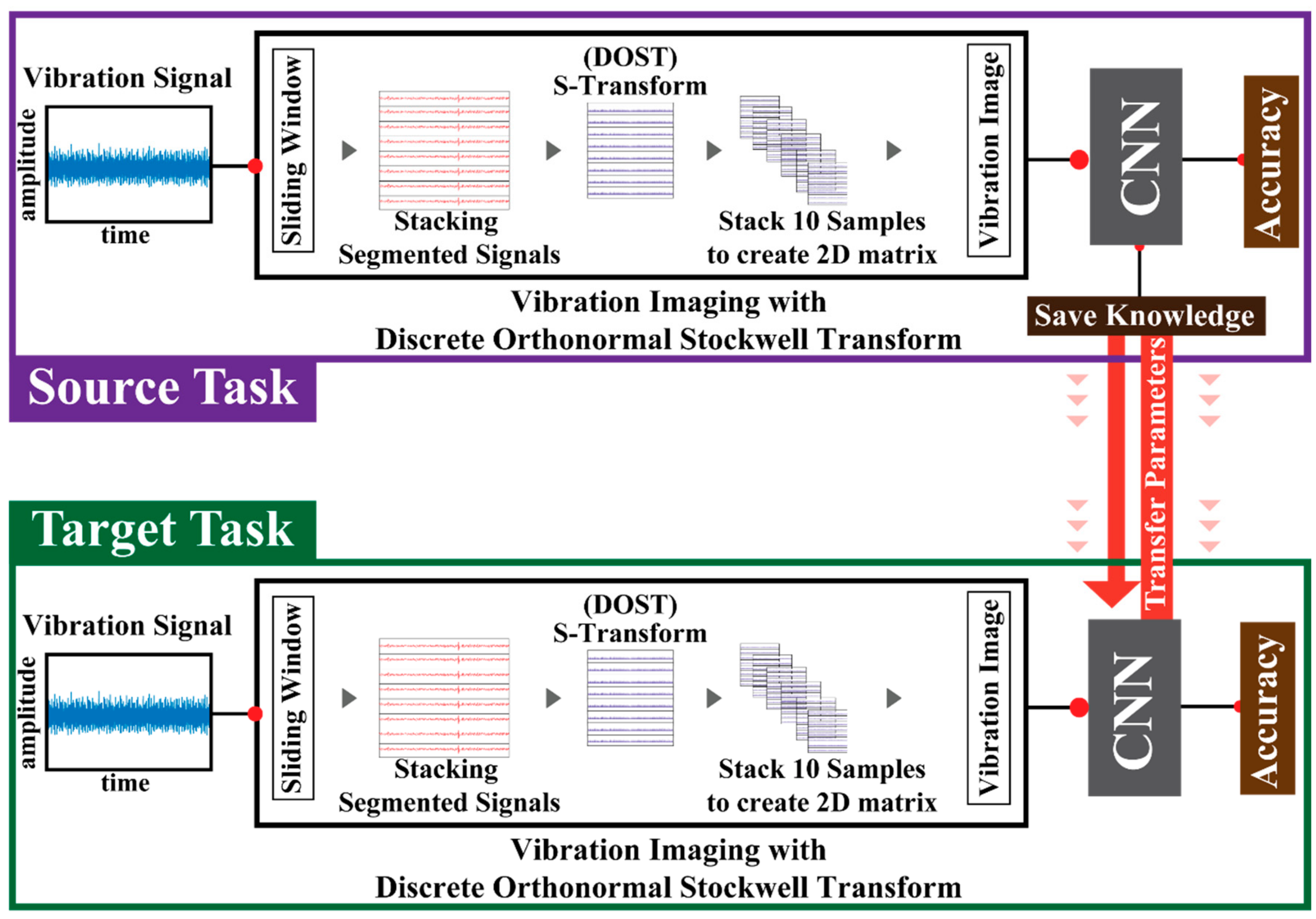
The proposed methodology mainly comprises three major tasks: (a) the source task, (b) the element transfer, and (c) the target task. The source and target tasks each have three common steps to use the convoluted layers of the proposed neural network architectures: (a) data input, (b) vibration imaging, and (c) using the convolutional neural network (CNN). Vibration imaging works as the preprocessing step for the input data to generate identical patterns, and the CNN is used to save and transfer knowledge between the source and target tasks to achieve the classification for the bearing fault diagnosis. Figure 1 illustrates the overall proposed mechanism.
2.1. Vibration Imaging Using Discrete Orthonormal Stockwell Transform (DOST)
In the transfer learning (TL), first, the network is trained with a working condition (source task) and then those learnings are passed to another working condition (target task). Processing the substantial amount of 1D vibrational data from sensors requires massive computational cost and time. Therefore, an adjustable sliding window frame [33] mechanism is adopted with the goal of (a) creating a massive amount of source data to train the network efficiently, and (b) handling the large amount of data for further processing to fit it to the proposed network.
If the total length of the acquired vibration signal is , then the total number of the samples is:
In Equation (1), is the length of a single frame, which is selected based on the experimental requirements. The step size is . The length of the vibration signal is fixed in this study. The overall process of adjusting the sliding window frame is shown in Figure 2.
With a 1D signal, it is very difficult to observe identical patterns for different health types. Moreover, in recent studies [33,34], preprocessing-free transfer learning is claimed. Even with the limited amount of data for mechanical machines, network learning for a transferring scenario remains questionable. Huge chunks of data having a lot of variations can help a network gather some intrinsic information. This kind of information can help to classify other mechanical sensors further. In this scenario, TL is used to resolve the issue of reducing time along with boosting performance. However, TL cannot resolve the challenges of raw signals alone since the open source data are incommensurate. Also, for additional white noise, the time-domain information is not always accurate. Rather, preprocessing can result in more robust performance if it uses the TL-based approach instead of classical deep learning because a limited portion of data facilitated with some additional information can help us adjust the network weights to learn more accurate intrinsic feature information for classification. Current study focuses mainly on this idea. A 1D raw signal suffers from the inability to create invariant identical scenarios. Two-dimensional imaging is developed to achieve ascendable feature engineering that processes heterogeneous data from systems with invariant working principles. In this study, discrete orthonormal Stockwell transform (DOST)-based stacking for vibration imaging is employed as a preprocessing step in the proposed approach.
The Stockwell transform (ST) was first proposed by R. G. Stockwell [30]. Using local spectral phase properties, it can represent time and frequency. The ST can distinctively combine a frequency-dependent resolution of the time–frequency space with unequivocally referenced local phase information. In other words, the ST is like a fusion between the Gabor transform and the wavelet transform. In practice, this time–frequency decomposition tool overcomes some of the drawbacks (i.e., provides better time–frequency resolution) of the short time Fourier transform (STFT). In [30], R. G. Stockwell described a method to decompose a signal on a discrete orthogonal basis for the ST (DOST basis). In this study, the DOST basis is considered to form 2D images with identical patterns. To perform the orthogonal transform, this method uses the discrete Fourier transform (DFT) [3].
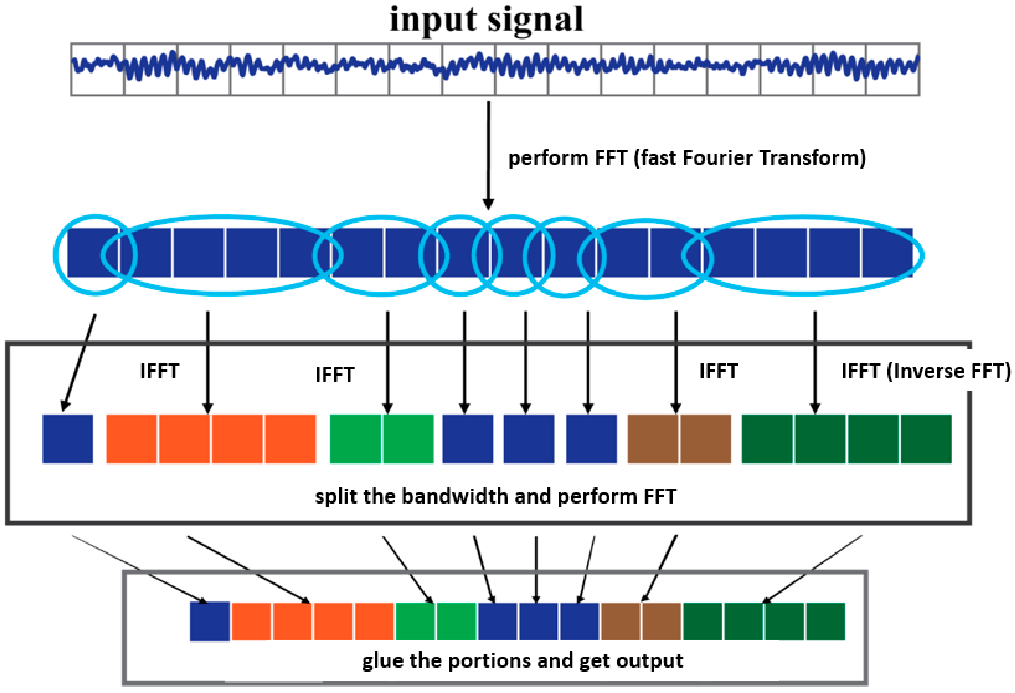
First, the method performs a fast Fourier transform on each segmented windowed sample. Then, it segments the processed signal via frequency partitioning for the DOST, that is, changing dyadic negative to positive. Next, on each bandwidth partition, it calculates the inverse Fourier transformation. Finally, it combines all these partitions together to form the final DOST output. Figure 3 shows the process of this DOST basis method.
If a 1D function of time for a constant frequency is represented as , then the continuous [30,35] ST of a function is:
Equation (2) demonstrates the change of the amplitude and phase for this frequency over time. In the discrete case, there are computational advantages to using the equivalent frequency domain definition of the ST. However, as R. G. Stockwell pointed out, standard ST is computationally expensive () [27].
In [36], U. Battisti et al. demonstrated that the DOST basis is not suited to a standard Gaussian window. Later, in [37], Y. Wang et al. proposed a fast algorithm for the ST with a time complexity of . U. Battisti et al., in [36], extended that work and provided an adapted basis to decompose the ST with a general admissible window. Let us consider a signal with finite energy, where . If is the window in , then the S-transform is:
where . In [32], U. Battisti et al. assumed that one could find such a basis of L2([0,1]), where will be dependent on choice. Then, can be expressed as:
where .
They proved that an orthonormal basis of can satisfy the condition that ST is local in time and frequency and has a fast computation algorithm of time complexity to compute the coefficients.
To form the identical patterns, the considered DOST basis output of the segmented signals of all the types are stacked together. These stacks of the preprocessed signals form identical patterns for each health type. When stacking a huge number of segmented signals, these images are large. To address this issue, heights of the stacked signal are fixed for generating identical images in the experiment. If the total number of segmented signals is and each segment has length , then the size of the image is (). This height is very large as well as challenging to feed to the proposed network. To generate small images, samples from the segmented samples (where and ) are considered. Then, all the resized images are bunched together and fed into the network. In this study, can generate good resolution. This can be larger but note that increasing reduces the total number of samples.
2.2. Transfer Learning with Convolutional Neural Network (CNN)
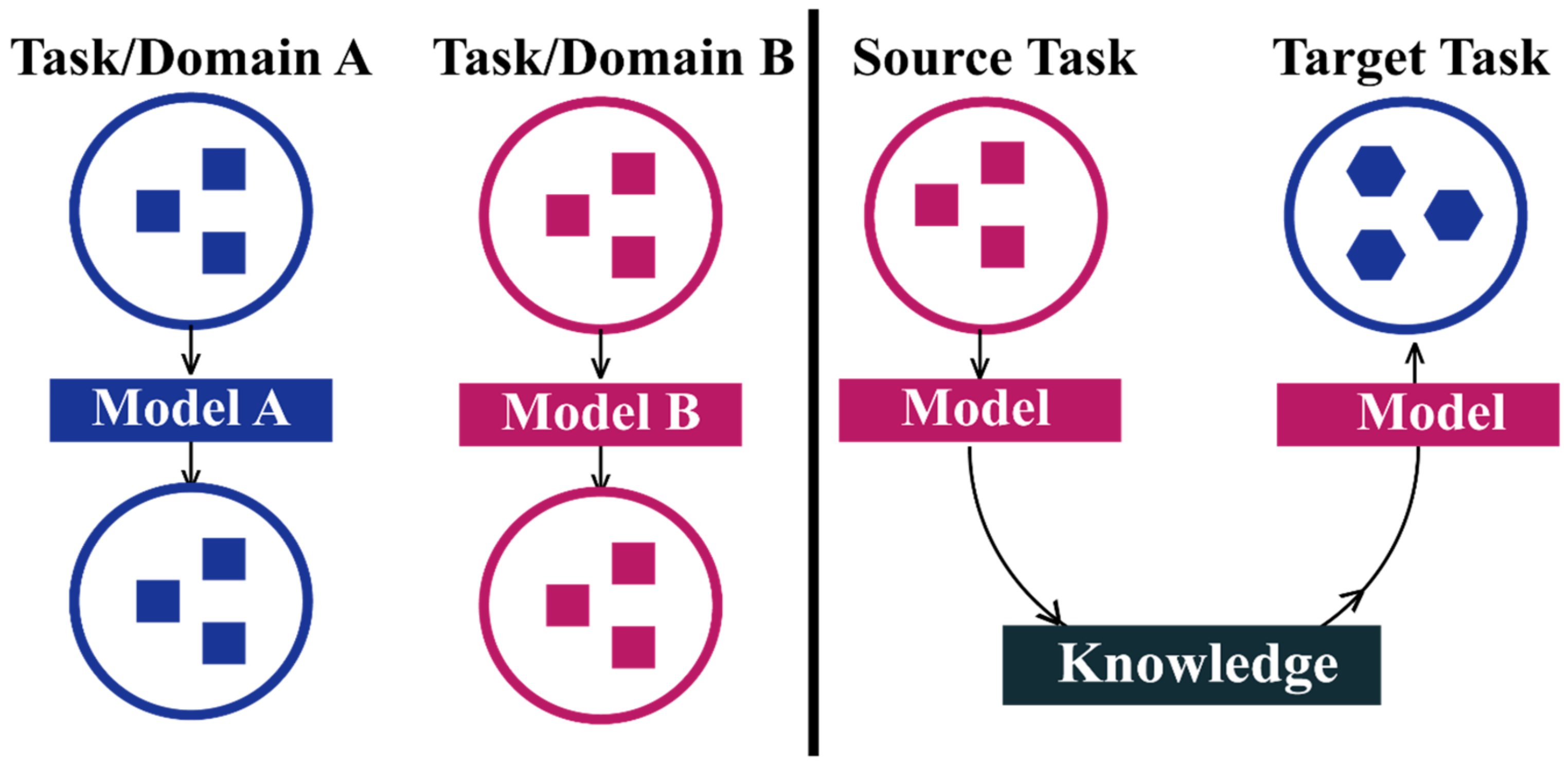
The prime goal of transfer learning (TL) is to improve the performance of a target task by using the knowledge from a source task. The source and target tasks may be similar or different. In this study, the source and target domains preserve similar types of feature spaces because the data types are similar except for the revolution speed of the bearings. In this study, transfer learning is employed to reduce the overhead of the training network. In practice, TL creates a robust fault diagnosis process [38]. Figure 4 illustrates the TL concept.
TL methods depend on machine-learning algorithms for learning the task. In this study, inductive learning is used. In inductive learning, TL is considered as a classifier along with one of the interference algorithms to solve classical classification problem (i.e., neural networks). These interference algorithms, that is, the deep neural networks, can automate the feature selection process through the hidden layers and then classify. In addition, they can preserve the knowledge of their learning and use it for further tasks. Convolutional neural networks (CNNs) have been considered as one of the most effective feed-forward supervised machine-learning networks. One more reason for considering CNN as the deep neural network for this study is that a large-scale CNN has the potential to be the most effective of the deep learning and classical methods. Moreover, using the transferred knowledge obtained from TL, with only a small set of training data, the large-scale CNN can achieve excellent performance in the considered scenarios [33,34,38].
A CNN is used to automate the detailed feature selection process for a given set of data, as well as to save the source knowledge for further usage in the target domain. A CNN has a hierarchical construction and collects from several convolutional, subsampling, and fully connected layers. This network makes optimal use of the indigenous connections (instead of fully-connected layers), weight distribution, and spatial or progressive subsampling to achieve invariance of shifting, scaling, and distortion in their inputs [39,40]. In this study, as TL and CNN are designed together, the learning of the well-trained layers are passed to the layers of the target network, where , and layer number denotes the output layer or last layer. Thus, the last layer of the target network is trained, providing an accuracy of output based on the learning from the source network [34].
For a mathematical, intuitive overview of the CNN, let and be the input and output vectors, respectively, for the network. The model has three layers—input, hidden and output layers—where the hidden vector is . The feed forward method is as follows:
where is the weight matrix between the input and hidden layers, is the weight matrix between the hidden and output layers, and represent the bias vector of the hidden and output layers, respectively, and is the sigmoid activation function. The loss function is as follows:
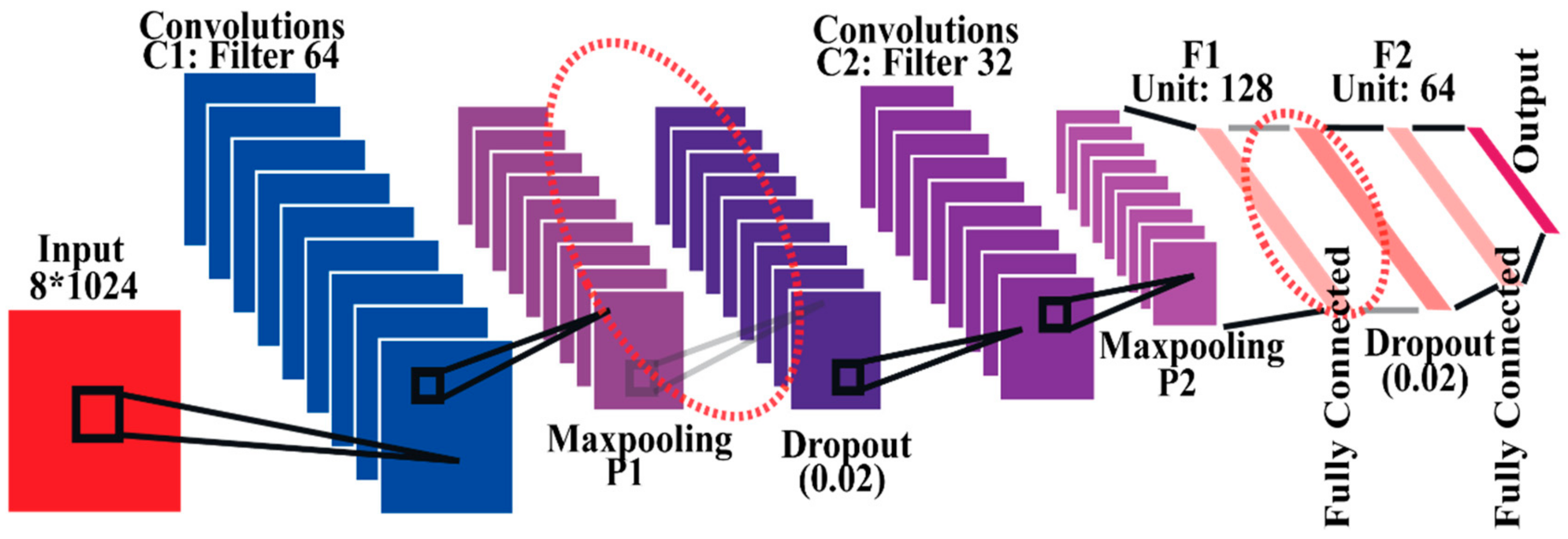
where represents the target vector and denotes the number of training samples. The aim of the CNN is to minimize the loss function through back propagation and gradient descent [33]. In this study, the architecture of the neural network contains nine layers along with one output layer (see Figure 5). From the convolution layer output, the max-pooling layer does the subsampling of data. A dropout layer is added to the network to avoid over-fitting. In this study, Adam optimizer is used for fine tuning the network and SoftMax classifier to improve the classification performance.
In the TL, the learning of these hidden layers is then passed to the target task to boost the learning of the target task. For the neural network, these learnings are stored in the form of weights. The layers that are transferred to the target network are listed in Table 1.
3. Result Analysis
3.1. Dataset and Experimental Working Conditions
To evaluate the proposed method, the publicly available seeded fault bearing dataset by Case Western Reserve University (CWRU) Bearing Data Center [41] is used. The data were accumulated by using a 2-horsepower (hp) Reliance Electric motor with a torque transducer and a dynamometer to apply different loads, ranging from 0 hp to 3 hp. Rotation velocities of the motor also varied from 1797 rpm to 1730 rpm. Drive end bearings were seeded with defects on the inner raceways, outer raceways, and rolling elements with the assistance of an electro-discharge machine, shown in Figure 6. The dataset consists of ratings of healthy condition (HC), inner raceway fault (IRF), ball fault (BF), and outer raceway fault (ORF) signals under the considered working conditions. The ORF has three variants: ORF at the center, ORF at the orthogonal, and ORF at the opposite positions. In this study, the variable length vibration acceleration signals were recorded at 12,000 samples/second (Hz) for the drive-end bearings.
To segment the signals by an adjustable sliding window, the proposed method considers 1024 data points for every frame. After that, the invariant conditions are established through vibration imagining via DOST-based stacking. As discussed earlier, after stacking, the dimension of an individual sample becomes . To evaluate the performance of this speed-invariant experiment, four different working conditions are considered. Under each set of working conditions, six different health types are included. Table 2 presents the details of the working conditions. In total, 300 fine-tuned epochs are revolved around the network for performance assessment.
3.2. Analysis of 2D Vibration Imaging
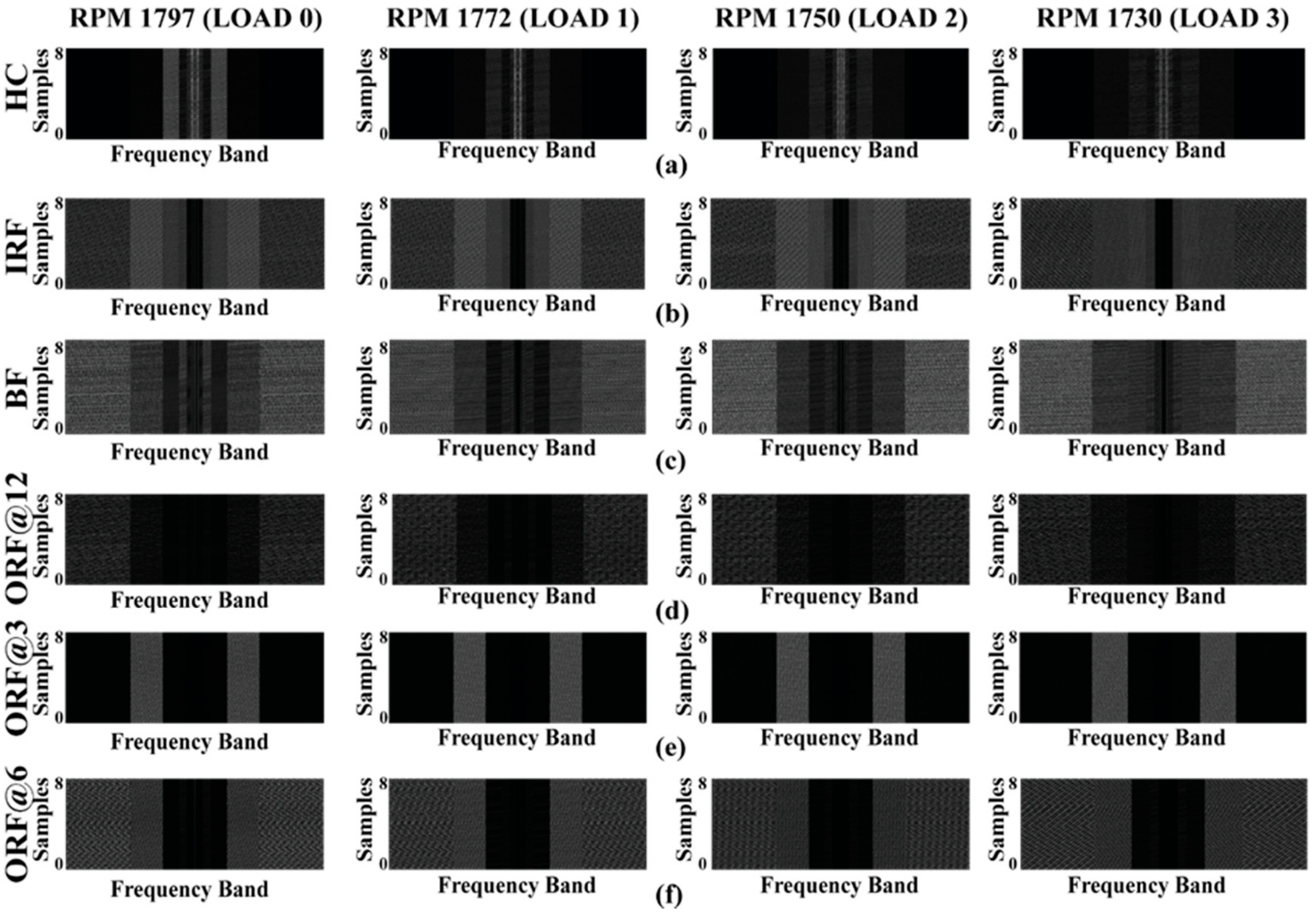
As described earlier, the reasons to employ 2D vibration imaging are as follows. One reason is to create an invariant scenario for different loads and rpms. For each health type (HC, IRF, BF, ORF at center, ORF at orthogonal and ORF at opposite), the 2D imaging exhibits identical patterns across working conditions. Another reason is to provide the CNN with the full advantages of the 2D structure with visibility of identical patterns. A further reason is be able to visually distinguish between the source and target domains to reduce negative transfer learning. Figure 7a–f shows the output of vibration imaging for each health type under different working conditions. Using the S-transform, the frequency domain is divided into several bandwidths, providing micropatterns based on bandwidth. From close observation, the rpm and load do not affect the identical patterns of the signals under different working conditions. Across different rpm and load levels, the pattern for each health condition does not vary, which demonstrates the similarity among all the working conditions for different health types.
3.3. Diagnostic Performance of the Proposed TL-Based Method
To validate the performance of the proposed TL-based method, the available data are divided into four different working conditions (WC), denoted WC 1, 2, 3, and 4 (described in Table 2). These datasets contain different speeds and loads, but the same type of health condition. The rpm invariance of this approach is validated by examining four separate scenarios. In the first scenario, WC 1 is used for training the network and saves the knowledge, and WC 2, 3, and 4 use that learning to perform the classification tests. From WC 2, 3, and 4, 10% of the data are used for adjusting the network to use the prior knowledge. In the second scenario, WC 2 is used for gathering the knowledge, and WC 2, 3, and 4 are used for TL-based testing. In the same manner, in Scenario 3, WC 3 is used for knowledge gathering, and in Scenario 4, WC 4 is used. The corresponding other working conditions are used for testing and classification. In each scenario, one dataset is known to the network, and the TL makes the later learning faster and more efficient, and achieves better accuracy. These tests validate the proposed approach. Table 3 lists the details of the diagnostic performance of the proposed approach.
To evaluate the performance of the proposed approach, the same experiment is also conducted with different amounts of training data. In this study, 80% of the training data are considered from the source dataset for each scenario (Table 2). With different percentages of training data, the overall classification accuracy varies as provided in Table 4. Table 4 clearly shows that the best performance is achieved when using 80% of the training data from the target dataset for the different scenarios.
In the Methodology section, Table 1 describes the proposed neural network architecture for TL. The table also shows which layers or stages are transferred to the target dataset for different scenarios to evaluate the performance. There are four stages in the network (Table 1), and the first three are transferred to perform TL. To evaluate the network’s performance, the number of stages is varied for transfer. In this study, 80% of data are used for training and the number of learning stages is only changed to evaluate the performance. Table 5 gives the overall performance results. As shown in Table 5, the proposed approach performs the best when Stages 1 to 3 (see Table 1) from the network are transferred to the target task.
3.4. Comparison Analysis
To evaluate the performance of the proposed approach, several experiments are performed with and without TL. In the experiment, WC 1 is considered as the source task and WC 2 as the target and the performance of WC 2 with transfer learning (WTL) and without transfer learning (NTL) is evaluated. The NTL scenario meant training the network from scratch (training:testing = 60:40) without transferring any knowledge from the source task. As shown in Table 6, the accuracy performance did not improve much for WTL versus NTL. For normal health type (HC), the accuracy is the same, and for the inner fault (IRF), the accuracy without TL is higher (2.2%). For the other health types, WTL performed better than NTL. On average, WTL provided 1.04% additional accuracy over NTL in this experimental scenario.
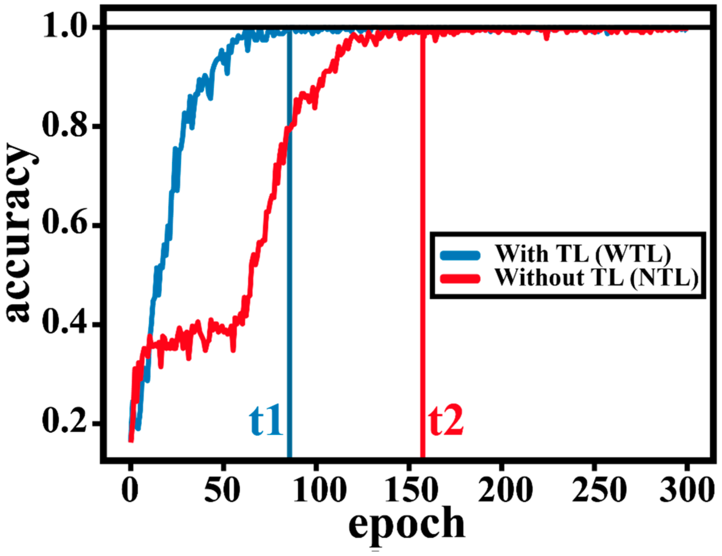
However, training time with TL is shorter than that without TL. As shown in Figure 8, the network provides the highest training accuracy (100%) with TL after almost 80 epochs (in t1 time), whereas NTL requires almost 160 epochs (in t2 time) to provide the same performance. These results demonstrate that transfer learning greatly reduces the training time while maintaining the overall performance.
To validate the performance of the proposed method, some recent deep learning approaches, including raw signal-based TL approach [33], hierarchical CNN-based approach [29], and ensemble deep autoencoders approach [27], are compared with the proposed method. In addition, the proposed TL-based network approach is compared with some of the classical machine learning approaches (e.g., SVM and ANN). These network architectures are analyzed with the same test scenarios to validate the performance improvement using the proposed TL-based CNN approach, as shown in Table 2. Table 7 shows the comparison results in detail for each scenario of the experiment, and our proposed approach outperforms conventional methods.
4. Conclusions
In this paper, a convolutional neural network–based transfer learning approach was proposed for automated feature extraction to improve the performance of bearing fault classification. To make the automated feature extraction more reliable and accurate, the discrete orthonormal Stockwell transform (DOST) was proposed as a preprocessing step for creating a load- and rpm-invariant scenario for considering signals of multiple health types. The theoretical and experimental analysis of this study demonstrated that TL boosts the performance of the network under invariant working conditions and brings the learning mechanism under one network architecture. The experimental analysis also established that DOST-based vibration imaging can help a two-dimensional CNN to learn features faster and with greater accuracy. Experimental results showed that the proposed method achieves an average of 99.8% classification accuracy for all health types (i.e., healthy condition, inner race fault, ball fault, and outer race fault for 1, 2, 3, and 6 o’clock sensor positions). In addition, the proposed method outperformed other state-of-the-art algorithms (i.e., ANN, SVM, hierarchical CNN, and deep autoencoders), showing 32.3%, 16.39%, 6.78% and 1.58% improvements in accuracy, respectively.
Author Contributions
All the authors contributed equally to the conception of the idea, implementing and analyzing the experimental results, and writing the manuscript.
Funding
This work was funded in part by the Korea Institute of Energy Technology Evaluation and Planning (KETEP) and the Ministry of Trade, Industry, & Energy (MOTIE) of the Republic of Korea (No. 20181510102160). It was also supported in part by the Ministry of SMEs and Startups (MSS), Korea, under the “Regional Specialized Industry Development Program (R&D, P006800689)” supervised by the Korea Institute for Advancement of Technology (KIAT), and in part by the Leading Human Resource Training Program of Regional Neo Industry through the National Research Foundation of Korea (NRF), funded by the Ministry of Science, ICT, and Future Planning (NRF-2016H1D5A1910564).
Conflicts of Interest
The authors declare no conflict of interest.
References
- Saidur, R. A review on electrical motors energy use and energy savings. Renew. Sustain. Energy Rev. 2010, 14, 877–898. [Google Scholar] [CrossRef]
- Khan, S.A.; Kim, J.M. Automated bearing fault diagnosis using 2d analysis of vibration acceleration signals under variable speed conditions. Shock Vib. 2016, 2016, 8729572. [Google Scholar] [CrossRef]
- El-Thalji, I.; Jantunen, E. Dynamic modelling of wear evolution in rolling bearings. Tribol. Int. 2015, 84, 90–99. [Google Scholar] [CrossRef]
- Zhang, R.; Peng, Z.; Wu, L.; Yao, B.; Guan, Y. Fault diagnosis from raw sensor data using deep neural networks considering temporal coherence. Sensors 2017, 17, 549. [Google Scholar] [CrossRef] [PubMed]
- Jiang, X.; Wu, L.; Ge, M. A novel faults diagnosis method for rolling element bearings based on ewt and ambiguity correlation classifiers. Entropy 2017, 19, 231. [Google Scholar] [CrossRef]
- Sohaib, M.; Kim, C.-H.; Kim, J.-M. A hybrid feature model and deep-learning-based bearing fault diagnosis. Sensors 2017, 17, 2876. [Google Scholar] [CrossRef] [PubMed]
- Li, S.; Liu, G.; Tang, X.; Lu, J.; Hu, J. An ensemble deep convolutional neural network model with improved d-s evidence fusion for bearing fault diagnosis. Sensors 2017, 17, 1729. [Google Scholar] [CrossRef] [PubMed]
- Thorsen, O.V.; Dalva, M. Failure identification and analysis for high-voltage induction motors in the petrochemical industry. IEEE Trans. Ind. Appl. 1999, 35, 810–818. [Google Scholar] [CrossRef]
- Tra, V.; Kim, J.; Khan, S.A.; Kim, J.-M. Incipient fault diagnosis in bearings under variable speed conditions using multiresolution analysis and a weighted committee machine. J. Acoust. Soc. Am. 2017, 142, EL35–EL41. [Google Scholar] [CrossRef] [PubMed] [Green Version]
- Jardine, A.K.S.; Lin, D.; Banjevic, D. A review on machinery diagnostics and prognostics implementing condition-based maintenance. Mech. Syst. Signal Process. 2006, 20, 1483–1510. [Google Scholar] [CrossRef]
- Mendizabal, X.; Arnaiz, A. Ball bearing damage detection using traditional signal processing algorithms. IEEE Instrum. Meas. Mag. 2013, 16, 20–25. [Google Scholar]
- Zhao, S.; Liang, L.; Xu, G.; Wang, J.; Zhang, W. Quantitative diagnosis of a spall-like fault of a rolling element bearing by empirical mode decomposition and the approximate entropy method. Mech. Syst. Signal Process. 2013, 40, 154–177. [Google Scholar] [CrossRef]
- Yin, S.; Ding, S.X.; Zhou, D. Diagnosis and prognosis for complicated industrial systems—Part I. IEEE Trans. Ind. Electron. 2016, 63, 2501–2505. [Google Scholar] [CrossRef]
- Yin, S.; Ding, S.X.; Zhou, D. Diagnosis and prognosis for complicated industrial systems—Part II. IEEE Trans. Ind. Electron. 2016, 63, 3201–3204. [Google Scholar] [CrossRef]
- Qin, X.; Li, Q.; Dong, X.; Lv, S. The fault diagnosis of rolling bearing based on ensemble empirical mode decomposition and random forest. Shock Vib. 2017, 2017, 2623081. [Google Scholar] [CrossRef]
- Huang, W.; Sun, H.; Wang, W. Resonance-based sparse signal decomposition and its application in mechanical fault diagnosis: A review. Sensors 2017, 17, 1279. [Google Scholar] [CrossRef] [PubMed]
- Duong, B.P.; Kim, J.M. Non-Mutually Exclusive Deep Neural Network Classifier for Combined Modes of Bearing Fault Diagnosis. Sensors 2018, 18, 1129. [Google Scholar] [CrossRef] [PubMed]
- Khan, S.A.; Kim, J.-M. Rotational speed invariant fault diagnosis in bearings using vibration signal imaging and local binary patterns. J. Acoust. Soc. Am. 2016, 139, EL100–EL104. [Google Scholar] [CrossRef] [PubMed]
- Soualhi, A.; Clerc, G.; Razik, H. Detection and diagnosis of faults in induction motor using an improved artificial ant clustering technique. IEEE Trans. Ind. Electron. 2013, 60, 4053–4062. [Google Scholar] [CrossRef]
- Kim, B.S.; Lee, S.H.; Lee, M.G.; Ni, J.; Song, J.Y.; Lee, C.W. A comparative study on damage detection in speed-up and coast-down process of grinding spindle-typed rotor-bearing system. J. Mater. Process. Technol. 2007, 187–188, 30–36. [Google Scholar] [CrossRef]
- Tahir, M.M.; Khan, A.Q.; Iqbal, N.; Hussain, A.; Badshah, S. Enhancing fault classification accuracy of ball bearing using central tendency based time domain features. IEEE Access 2017, 5, 72–83. [Google Scholar] [CrossRef]
- Huo, Z.; Zhang, Y.; Francq, P.; Shu, L.; Huang, J. Incipient fault diagnosis in roller bearing using optimized wavelet transform based on multi-speed vibration signatures. IEEE Access 2017, 5, 19442–19456. [Google Scholar] [CrossRef]
- Wang, W.; Lee, H. An energy kurtosis demodulation technique for signal denoising and bearing fault detection. Meas. Sci. Technol. 2013, 24, 025601. [Google Scholar] [CrossRef]
- Yang, Y. A signal theoretic approach for envelope analysis of real-valued signals. IEEE Access 2017, 5, 5623–5630. [Google Scholar] [CrossRef]
- Sugumaran, V.; Ramachandran, K.I. Effect of number of features on classification of roller bearing faults using svm and psvm. Expert Syst. Appl. 2011, 38, 4088–4096. [Google Scholar] [CrossRef]
- Saimurugan, M.; Ramachandran, K.I.; Sugumaran, V.; Sakthivel, N.R. Multi component fault diagnosis of rotational mechanical system based on decision tree and support vector machine. Expert Syst. Appl. 2011, 38, 3819–3826. [Google Scholar] [CrossRef]
- Shao, H.; Jiang, H.; Lin, Y.; Li, X. A novel method for intelligent fault diagnosis of rolling bearings using ensemble deep auto-encoders. Mech. Syst. Signal Process. 2018, 102, 278–297. [Google Scholar] [CrossRef]
- Sohaib, M.; Kim, J.-M. Reliable fault diagnosis of rotary machine bearings using a stacked sparse autoencoder-based deep neural network. Shock Vib. 2018, 2018, 2919637. [Google Scholar] [CrossRef]
- Lu, C.; Wang, Z.; Zhou, B. Intelligent fault diagnosis of rolling bearing using hierarchical convolutional network based health state classification. Adv. Eng. Inform. 2017, 32, 139–151. [Google Scholar] [CrossRef]
- Stockwell, R.G. A basis for efficient representation of the s-transform. Digit. Signal Process. Rev. J. 2007, 17, 371–393. [Google Scholar] [CrossRef]
- Appana, D.K.; Ahmad, W.; Kim, J.-M. Speed invariant bearing fault characterization using convolutional neural networks. In Multi-Disciplinary Trends in Artificial Intelligence; Phon-Amnuaisuk, S., Ang, S.-P., Lee, S.-Y., Eds.; Springer International Publishing: Cham, Switzerland, 2017; pp. 189–198. [Google Scholar]
- Malek, S.; Melgani, F.; Bazi, Y. One-dimensional convolutional neural networks for spectroscopic signal regression. J. Chemom. 2018, 32, e2977. [Google Scholar] [CrossRef]
- Zhang, R.; Tao, H.; Wu, L.; Guan, Y. Transfer learning with neural networks for bearing fault diagnosis in changing working conditions. IEEE Access 2017, 5, 14347–14357. [Google Scholar] [CrossRef]
- Cao, P.; Zhang, S.; Tang, J. Preprocessing-free gear fault diagnosis using small datasets with deep convolutional neural network-based transfer learning. IEEE Access 2018, 6, 26241–26253. [Google Scholar] [CrossRef]
- Stockwell, R.G.; Mansinha, L.; Lowe, R.P. Localization of the complex spectrum: The s transform. IEEE Trans. Signal Process. 1996, 44, 998–1001. [Google Scholar] [CrossRef]
- Battisti, U.; Riba, L. Window-dependent bases for efficient representations of the stockwell transform. Appl. Comput. Harmonic Anal. 2016, 40, 292–320. [Google Scholar] [CrossRef]
- Kaba, M.D.; Camlibel, M.K.; Wang, Y.; Orchard, J. Fast discrete orthonormal stockwell transform. SIAM J. Sci. Comput. 2009, 31, 4000–4012. [Google Scholar]
- Shie, C.-K.; Chuang, C.-H.; Chou, C.-N.; Wu, M.-H.; Chang, E.Y. Transfer representation learning for medical image analysis. In Proceedings of the 37th Annual International Conference of the IEEE Engineering in Medicine and Biology Society (EMBC), Milano, Italy, 25–29 August 2015. [Google Scholar]
- LeCun, Y.; Bottou, L.; Bengio, Y.; Haffner, P. Gradient-based learning applied to document recognition. Proc. IEEE 1998, 86, 2278–2323. [Google Scholar] [CrossRef]
- Tra, V.; Kim, J.; Khan, S.A.; Kim, J.-M. Bearing fault diagnosis under variable speed using convolutional neural networks and the stochastic diagonal levenberg-marquardt algorithm. Sensors 2017, 17, 2834. [Google Scholar] [CrossRef] [PubMed]
- Case Western Reserve University. Bearing Data Center Website. Available online: https://csegroups.case.edu/bearingdatacenter/pages/welcome-case-western-reserve-university-bearing-data-center-website (accessed on 13 July 2018).
Figure 1.
Detailed process of the proposed method.

Figure 2.
Adjustable sliding window technique.
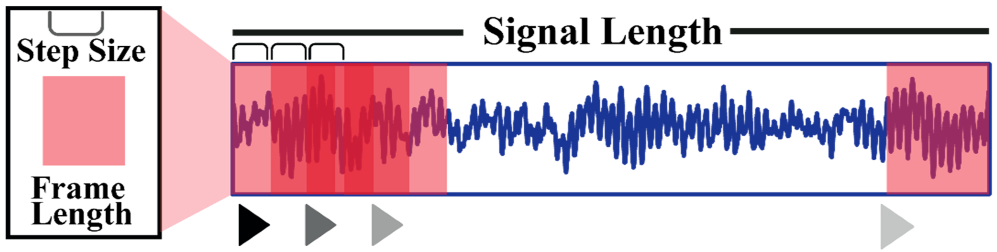
Figure 3.
Discrete orthonormal Stockwell transform (DOST) basis construction process, where FFT stands for fast Fourier transform.
Figure 3.
Discrete orthonormal Stockwell transform (DOST) basis construction process, where FFT stands for fast Fourier transform.

Figure 4.
The left side shows the conventional learning process, while the right side shows the concept of transfer learning (TL).
Figure 4.
The left side shows the conventional learning process, while the right side shows the concept of transfer learning (TL).

Figure 5.
Proposed architecture of the 2D CNN.

Figure 6.
An overview of the experimental setup.
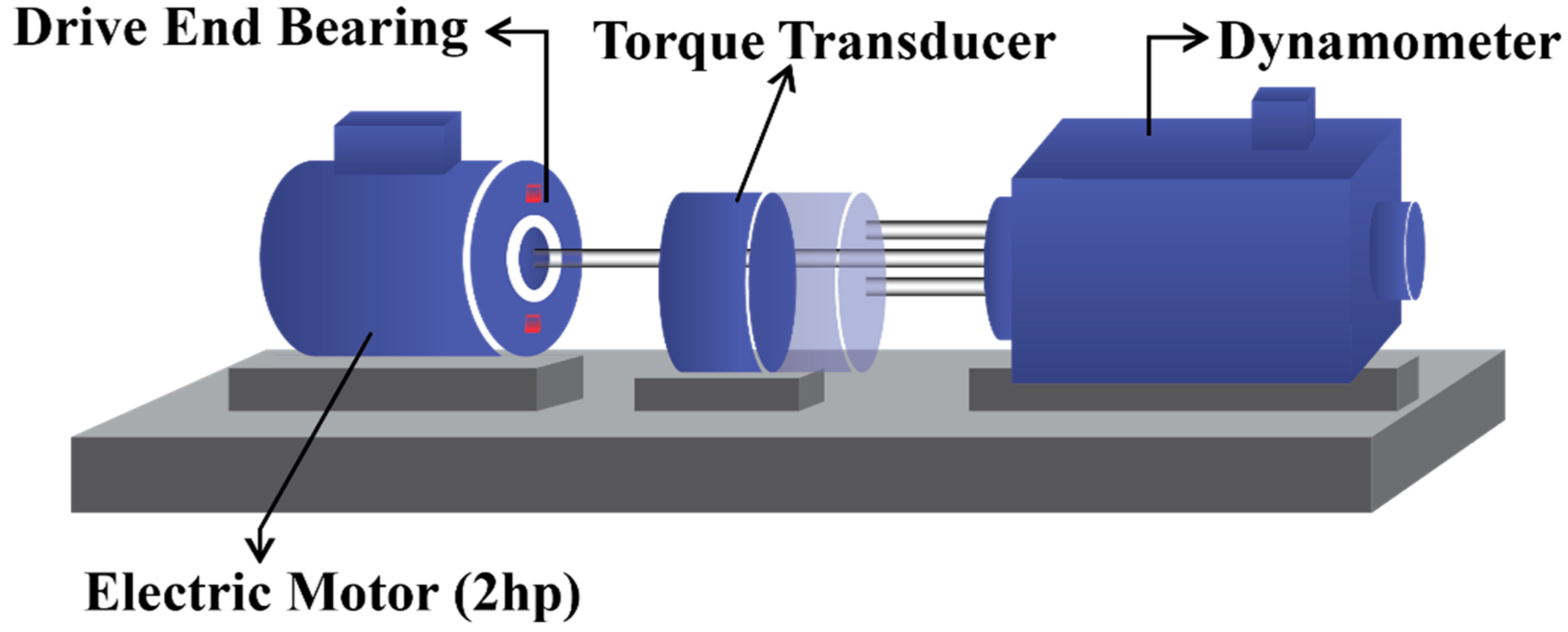
Figure 7.
Vibration images based on DOST for different health conditions. (a) HC (Healthy Condition), (b) IRF (Inner Race Fault), (c) BF (Ball Fault), (d) ORF (Outer Race Fault), and (f) ORF at opposite position.
Figure 7.
Vibration images based on DOST for different health conditions. (a) HC (Healthy Condition), (b) IRF (Inner Race Fault), (c) BF (Ball Fault), (d) ORF (Outer Race Fault), and (f) ORF at opposite position.

Figure 8.
Training accuracy comparison with and without transfer learning.

Table 1.
Proposed architecture of the CNN for transfer specification for target network.
| Stage | Stage Specification | Layer No. | Layer Name in Network | Transfer |
|---|---|---|---|---|
| 1 | Training stage | 01 | Convolutional | Yes |
| 02 | Maxpooling | Yes | ||
| 03 | Dropout | Yes | ||
| 2 | Training stage | 04 | Convolutional | Yes |
| 05 | Maxpooling | Yes | ||
| 06 | Fully connected | Yes | ||
| 3 | Training stage | 07 | Dropout | Yes |
| 08 | Fully connected | Yes | ||
| 4 | Output stage | 09 | Fully connected | No |
Table 2.
Details of the considered working conditions with the same health types.
| Fs = 12 kHZ | Health Type | Motor Load | Motor Speed | Crack Size |
|---|---|---|---|---|
| Diameter (Inches) | ||||
| Working Condition 1 | Healthy Condition (HC) | 0 | 1797 Rounds/min | Nil |
| Inner Race Fault (IRF) | 0 | 1797 Rounds/ min | 0.007 | |
| Ball Fault (BF) | 0 | 1797 Rounds/min | 0.007 | |
| Outer Race Fault at center (ORF@12) | 0 | 1797 Rounds/min | 0.007 | |
| Outer Race Fault at orthogonal (ORF@3) | 0 | 1797 Rounds/min | 0.007 | |
| Outer Race Fault at opposite (ORF@6) | 0 | 1797 Rounds/min | 0.007 | |
| Working Condition 2 | Healthy Condition (HC) | 1 | 1772 Rounds/min | Nil |
| Inner Race Fault (IRF) | 1 | 1772 Rounds/min | 0.007 | |
| Ball Fault (BF) | 1 | 1772 Rounds/min | 0.007 | |
| Outer Race Fault at center (ORF@12) | 1 | 1772 Rounds/min | 0.007 | |
| Outer Race Fault at orthogonal (ORF@3) | 1 | 1772 Rounds/min | 0.007 | |
| Outer Race Fault at opposite (ORF@6) | 1 | 1772 Rounds/min | 0.007 | |
| Working Condition 3 | Healthy Condition (HC) | 2 | 1750 Rounds/min | Nil |
| Inner Race Fault (IRF) | 2 | 1750 Rounds/min | 0.007 | |
| Ball Fault (BF) | 2 | 1750 Rounds/min | 0.007 | |
| Outer Race Fault at center (ORF@12) | 2 | 1750 Rounds/min | 0.007 | |
| Outer Race Fault at orthogonal (ORF@3) | 2 | 1750 Rounds/min | 0.007 | |
| Outer Race Fault at opposite (ORF@6) | 2 | 1750 Rounds/min | 0.007 | |
| Working Condition 4 | Healthy Condition (HC) | 3 | 1730 Rounds/min | Nil |
| Inner Race Fault (IRF) | 3 | 1730 Rounds/min | 0.007 | |
| Ball Fault (BF) | 3 | 1730 Rounds/min | 0.007 | |
| Outer Race Fault at center (ORF@12) | 3 | 1730 Rounds/min | 0.007 | |
| Outer Race Fault at orthogonal (ORF@3) | 3 | 1730 Rounds/min | 0.007 | |
| Outer Race Fault at opposite (ORF@6) | 3 | 1730 Rounds/min | 0.007 |
Table 3.
Diagnostic performance of the proposed model under different scenarios.
| Scenario | Source Dataset | Target Dataset | Classification Accuracy (%) | Average Classification Accuracy (%) | Overall Classification Accuracy (%) | |||||
|---|---|---|---|---|---|---|---|---|---|---|
| HC | IRF | BF | ORF@12 | ORF@3 | ORF@6 | |||||
| 1 | WC 1 | WC 2 | 100 | 100 | 100 | 100 | 100 | 100 | 100 | 99.99 |
| WC 3 | 100 | 100 | 100 | 100 | 100 | 100 | 100 | |||
| WC 4 | 100 | 99.88 | 100 | 100 | 100 | 100 | 99.98 | |||
| 2 | WC 2 | WC 1 | 100 | 100 | 100 | 100 | 100 | 100 | 100 | 99.98 |
| WC 3 | 100 | 100 | 100 | 100 | 100 | 100 | 100 | |||
| WC 4 | 100 | 100 | 100 | 99.69 | 100 | 100 | 99.95 | |||
| 3 | WC 3 | WC 1 | 100 | 100 | 100 | 100 | 100 | 100 | 100 | 99.90 |
| WC 2 | 100 | 100 | 100 | 98.44 | 100 | 100 | 99.74 | |||
| WC 4 | 100 | 99.83 | 100 | 100 | 100 | 100 | 99.97 | |||
| 4 | WC 4 | WC 1 | 99.94 | 98.68 | 99.47 | 100 | 99.92 | 99.29 | 99.55 | 99.54 |
| WC 2 | 99.96 | 99.73 | 100 | 99.63 | 99.68 | 99.57 | 99.76 | |||
| WC 3 | 99.98 | 98.22 | 100 | 98.37 | 99.53 | 99.79 | 99.32 | |||
| Average Accuracy (%) | 99.99 | 99.95 | 99.96 | 99.68 | 99.93 | 99.89 | 99.86 | 99.85 | ||
Table 4.
Classification results for different sizes of training data.
| Scenario | Overall Classification Accuracy (%) | |||
|---|---|---|---|---|
| Training Data 80% | Training Data 60% | Training Data 40% | Training Data 20% | |
| 1 | 99.99 | 96.44 | 86.22 | 79.18 |
| 2 | 99.98 | 96.23 | 86.45 | 77.43 |
| 3 | 99.90 | 95.82 | 85.32 | 77.92 |
| 4 | 99.54 | 95.59 | 83.96 | 67.11 |
Table 5.
Impact on overall classification accuracy of different numbers of stages for TL.
| Scenario | Overall Classification Accuracy with Transfer Learning (TL) (%) | ||
|---|---|---|---|
| Transfer Stages 1–3 | Transfer Stages 1–2 | Transfer Stage 1 | |
| 1 | 99.99 | 93.44 | 79.61 |
| 2 | 99.98 | 93.31 | 79.22 |
| 3 | 99.90 | 93.49 | 78.13 |
| 4 | 99.54 | 92.61 | 77.29 |
Table 6.
Comparison analysis of the classification accuracies of transfer learning-based model (WTL) vs. without transfer learning (NTL).
Table 6.
Comparison analysis of the classification accuracies of transfer learning-based model (WTL) vs. without transfer learning (NTL).
| Health Types | WTL (%) | NTL (%) | Improvements (%) |
|---|---|---|---|
| HC | 100 | 100 | 0 |
| IRF | 95.72 | 97.92 | −2.2 |
| BF | 96.22 | 95.2 | 1.02 |
| ORF@12 | 96.79 | 93.41 | 3.38 |
| ORF@3 | 97.21 | 94.90 | 2.31 |
| ORF@6 | 93.11 | 91.39 | 1.72 |
| Overall | 96.51 | 95.47 | 1.04 |
Table 7.
Comparison of classification accuracy (proposed vs. existing methods).
| Scenario | Method | Classification Accuracy (%) | Average Accuracy (%) | Improvement (%) [Proposed Method] | |||||
|---|---|---|---|---|---|---|---|---|---|
| HC | IRF | BF | ORF@12 | ORF@3 | ORF@6 | ||||
| 1 | ANN | 70.29 | 68.22 | 67.45 | 64.92 | 65.79 | 67.39 | 67.34 | 32.65 |
| SVM | 82.43 | 80.33 | 83.22 | 85.29 | 81.22 | 80.19 | 82.11 | 17.88 | |
| [29] | 93.44 | 93.2 | 93.79 | 93.72 | 92.69 | 92.44 | 93.21 | 6.78 | |
| [27] | 97.22 | 97.39 | 98.2 | 97.93 | 97.51 | 97.63 | 97.65 | 2.34 | |
| [33] | 100 | 93.2 | 96.45 | 94.2 | 94 | 93.55 | 95.23 | 4.76 | |
| Proposed | 100 | 99.96 | 100 | 100 | 100 | 100 | 99.99 | - | |
| 2 | ANN | 70.11 | 69.9 | 67.96 | 64.11 | 64.7 | 67.49 | 67.38 | 32.60 |
| SVM | 81.9 | 82.3 | 82.57 | 85.39 | 81.83 | 81.29 | 82.55 | 17.43 | |
| [29] | 93.39 | 93.86 | 93.5 | 93.29 | 92.98 | 92.95 | 93.33 | 6.65 | |
| [27] | 97.86 | 97.19 | 97.49 | 97.3 | 97.59 | 97.77 | 97.53 | 2.45 | |
| [33] | 100 | 93.2 | 96.45 | 94.2 | 94 | 93.55 | 95.28 | 4.7 | |
| Proposed | 100 | 99.96 | 100 | 100 | 100 | 100 | 99.98 | - | |
| 3 | ANN | 69.3 | 67.22 | 67.1 | 64.92 | 64.6 | 66.13 | 66.55 | 32.31 |
| SVM | 82.72 | 82.9 | 83.17 | 86.22 | 83.2 | 82.57 | 83.46 | 16.39 | |
| [29] | 92.63 | 93.12 | 92.86 | 92.77 | 92.09 | 92.13 | 92.6 | 7.25 | |
| [27] | 97.1 | 96.33 | 97.78 | 97.5 | 97.61 | 97.21 | 97.26 | 2.6 | |
| [33] | 100 | 93.2 | 96.45 | 94.2 | 94 | 93.55 | 95.26 | 4.59 | |
| Proposed | 100 | 99.96 | 100 | 100 | 100 | 100 | 99.85 | - | |
| 4 | ANN | 67.2 | 66.9 | 65.3 | 63.82 | 64.9 | 63.92 | 65.34 | 34.2 |
| SVM | 80.1 | 81.95 | 82.3 | 84.29 | 81.22 | 79.49 | 81.56 | 17.98 | |
| [29] | 93.87 | 92.91 | 92.94 | 92.7 | 91.19 | 91.73 | 92.56 | 6.98 | |
| [27] | 97.89 | 97.94 | 98.92 | 97.61 | 97.49 | 97.89 | 97.96 | 1.58 | |
| [33] | 100 | 93.2 | 96.45 | 94.2 | 94 | 93.55 | 94.45 | 5.09 | |
| Proposed | 100 | 99.96 | 100 | 100 | 100 | 100 | 99.54 | - | |
© 2018 by the authors. Licensee MDPI, Basel, Switzerland. This article is an open access article distributed under the terms and conditions of the Creative Commons Attribution (CC BY) license (http://creativecommons.org/licenses/by/4.0/).
Share and Cite
MDPI and ACS Style
Hasan, M.J.; Kim, J.-M. Bearing Fault Diagnosis under Variable Rotational Speeds Using Stockwell Transform-Based Vibration Imaging and Transfer Learning. Appl. Sci. 2018, 8, 2357. https://doi.org/10.3390/app8122357
AMA Style
Hasan MJ, Kim J-M. Bearing Fault Diagnosis under Variable Rotational Speeds Using Stockwell Transform-Based Vibration Imaging and Transfer Learning. Applied Sciences. 2018; 8(12):2357. https://doi.org/10.3390/app8122357
Chicago/Turabian StyleHasan, Md Junayed, and Jong-Myon Kim. 2018. "Bearing Fault Diagnosis under Variable Rotational Speeds Using Stockwell Transform-Based Vibration Imaging and Transfer Learning" Applied Sciences 8, no. 12: 2357. https://doi.org/10.3390/app8122357
Note that from the first issue of 2016, this journal uses article numbers instead of page numbers. See further details here.