1. Introduction
Besides high product quality, total cost and response time seem to be the key success factors to be optimized in Logistics Process (LP) in order to be more competitive in the global markets [
1]. Therefore, in today environment the organizations cannot afford to keep the LP within traditional frameworks, which consider a high Finished Good (FG) inventory level and slow response times [
2]. Consequently, organizations should consider and incorporate strategies to improve organizational performance by reducing costs and achieving excellence in the LP [
3]. Lean manufacturing tools and techniques used to reduce waste in the processes, such as just-in-time and inventory management [
4].
Logistics cost has an important role in the organizations, being that worldwide cost of LP represents between 9% and 20% of Gross Domestic Product; the variation depends on the region where the process is carried out [
5]. As shown by research conducted by [
6], the average cost to carry out LP in Latin America is 18.6% of the total cost of sales. However, some Latin America countries are above average, as is the case of Mexico, where the average cost constitutes a 21%. Therefore, it can be concluded that there is a great opportunity to optimize LP in the Mexican enterprises, because on average, almost a quarter of the selling price to the consumer is used in this activity [
6].
The inventory management and transportation are two of the main logistical costs in the electronics industry [
7]. In logistics, optimization is used for different purposes, such as minimizing Total Logistics Cost (TLC). For the case study presented in this paper, which was implemented in the electronic industrial cluster, the purpose is to improve TLC. In the other hand, constraints to achieve this objective are: Inventory Carrying Cost (ICC), which is related to the storage and maintenance of the inventory during a certain period of time; Response Time Cost (RTC), this is associated with the fulfillment of the committed customer service response time in order to avoid penalties; and Lost Sales Cost, it is a profit or income foregone due to customer orders could not be fulfilled (LSC), [
1]. Therefore, Minimizing TLC is a balance achieved among the ICC, RTC and LSC, where define optimal inventory level is key in order to achieve this activity, TLC is represented by the mathematical Equation (1).
Optimization of TLC can be achieved with the application of analytical models and simulation. However, LP is categorized as a complex system and it is difficult to study it via analytical models. On the other hand, simulation is considered a powerful tool for comparing alternatives for decision-making; and due to the stochastic nature of this technique, an efficient comparison needs to consider the application of statistical techniques for a better analysis [
8]. Those concepts are presented in a friendly manner in this study with the application of commercial software to design the simulation model that represents virtually the real life of LP and to run the statistical analysis with the RSM technique.
The present case study, considers LP is performed under traditional framework; where, the majority of FG inventory is concentrated in a Distribution Center (DC) in Mexico City, which is 1750 miles from the manufacturing plant, in order to supply product to wholesale customers located in different cities of Mexico. Therefore, this study aims to test the following hypothesis: “stochastics tools can be used to define strategies that help to improve TLC without affecting customer service.”
Logistics and the TV Manufacturing Industry in the Northern Border of Mexico
Despite the logistics hurdles, the Mexican TV manufacturing role has been in constant evolution since the first Asian-owned factories began operations. About 1.7 million TV sets for the U.S. market were produced in Mexico in 1987 [
9]. By 1998, the output was 19.1 million, about 25. Six million in 2003 and peaked at nearly 40 million sets in 2012, with most of the production coming from the regions around Tijuana and Mexicali in Mexico [
10].
Although the state of Baja California has a strategic location in the Northern Border of Mexico for the TV manufacturing industry, there are weaknesses in the logistics process to supply finished good products to the local market. The Mexican TV sales in 2013 were 6.3 million, which represents around 15% of total local production so the remaining 85% is for exporting [
11]. However, the logistics process for the local market is performed with the traditional framework, while for the exporting market the best practices are applied.
This research is organized as follow
Section 2 focuses on the literature review to analyze recent contributions in the field of lean logistics.
Section 3 describes how the case study methodology was applied in three phases: collect information, build a discrete event simulation model and statistical method for optimization.
Section 4 focuses on presents the application of the case study for the logistic process optimization of a television manufacturing company that supply finished good from two distribution centers to their customers; this as a result of this research the empirical mathematical model that allows making estimation is defined and it is tested with different targets. In
Section 5 conclusions are commented remarking the importance that Stochastics methods have for optimization purpose.
2. Literature Review
In the process of supply chain planning, logistics is a fundamental part; due to the activities involved: implementing and controlling the flow and storage of goods, services and information in an efficient way to meet customer requirements. Lean logistics applies lean manufacturing thinking to control logistics activities. The implementation of lean manufacturing strategies, tools and techniques into logistic operations has brought advantages such as costs and product waste reduction, while improving productivity, efficiency, quality and delivery, as well as satisfying customers and employees [
4,
12,
13,
14,
15].
The goal of Lean Manufacturing is to control, reduce and even eliminate waste, at the right time, in the right place, providing the right amount of product. The logistics waste consists of inventory, waiting, overproduction, overprocessing, defect, motion and transportation, respectively considered from greater to lesser impact on costs [
16,
17]. Lean logistics highlights customers first; timely, accurate and overall optimization; continuous improvement and innovative ideas. Lean logistics system planning and design can be divided into two submodules: material flow and information flow. To analyze the material flow and information flow cross the company, Value Stream Map (VSM) is used [
18]. The improvements in the system can be achieved through optimization strategies related to logistics process, logistics organization structure, logistic operation, standardization and logistics management, logistic professional personnel, logistics cost management and logistics performance evolution. In a study conducted with companies registered in the Singapore Logistics Association, it was found that 37.5% has implemented lean tools in the development of its operations [
19]. Finally, there are optimization techniques for optimization of LP that are discussed in the next section.
2.1. Techniques for Optimization in Logistics
Traditional framework to perform the logistics process, it is to maintain FG high inventories to ensure customer satisfaction and avoid lost sales costs. However, maintaining high inventories hides many inefficiencies in the activities for this process, which are directly reflected in the logistics cost. By this reason, leading companies apply best practices, such as direct store deliveries, which dramatically reduce inventory levels and cycle times in product distribution [
20].
Rossini and Portioli [
21] analyze the impact of using different supply chain planning models and propose the approach to use is depending on the conditions. A structured framework for comparison and evaluation of supply chain planning models under different conditions had been provided, including external transportation costs. Future research must include improvements in shipment rules may allow Lean Production to improve its transportation performance. In this simulation study, a simple general shipment rule of minimum truck saturation had been applied. They recommend further studies analyzing more complex rules that can increase efficiency of transportation, as milk-run or compound deliveries. Likewise, a simulation study on a multi-product supply chain could lead to more insights on the potential of lean approach adoption along the supply chain.
Regarding to environmental impact Ugarte et al. [
4] tested the hypotheses that since just-in-time inventory management significantly increases the frequency of transport it will also increase greenhouse gas emissions in a supply chain; this by using a simulation model of a manufacturing- retailer supply chain. They used a discrete event simulation model of a two-echelon supply-chain composed of distribution and retailing operations to test the hypotheses. The model included fixed infrastructural elements in the warehousing and retailing facilities, while integrating mobile infrastructural elements in the form of transportation of goods from the warehouse to the retailing facility and the corresponding backhauling operations. In a parallel way, Guo et al. [
22] proposed a timed colored Petri net simulation-based self-adaptive collaboration method for Internet of Things-enabled production-logistics systems. They combined the schedule of token sequences in the timed colored Petri net with real-time status of key production and logistics equipment. The key equipment is made ‘smart’ to actively publish or request logistics tasks. A simulation experiment was conducted to validate the performance and applicability of the proposed method and computational experiments demonstrate that the proposed method outperforms the event-driven method in terms of reductions of waiting time, makespan and electricity consumption. This proposed method could be applicable to other manufacturing systems to implement production-logistics collaboration. In this way, Papoutsis et al. [
23] conducted a sustainability analysis of concrete innovative and already tested retail logistics solutions addressing the research question “what are the effects of retail logistics solutions on total costs and sustainability performance?” For the analysis, they developed and applied an indicator-based framework based on the key sustainability components (economy, environment, society) and enriched by the addition of the transport component. External costs analysis showed that higher degree of internalization is achieved in the line-haul transport. As a conclusion, they affirmed the impact of innovative and already tested solutions relies on a variety of factors: organizational, urban context, type of goods transported, engagement of stakeholders and so forth. So that, innovation is crucial for urban retail logistics impacting on transport service, society, economy and environment.
Ji et al. [
24] proposed the scheduling problem in the context of a three-stage supply chain comprising a supplier, a manufacturer and a customer. The objective was to minimize the sum of the total weighted inventory cost and transport cost. They provided Fully Polynomial-Time Approximation Schemes (FPTAS) algorithm without considering the weight of the inventory cost for each for four cases of the batching and scheduling problem that considers the job. In comparison, they first introduced the weighted parameter in this weighted inventory cost. They concluded the transport cost is related to the number of batches created.
Ndhaief, Bistorin and Rezg [
25] improved a distribution plan supporting an urban distribution center (UDC) to solve the last mile problem of urban freight. They defined a mathematical model for searching the best distribution and maintenance plans using a subcontracting strategy; they considered delay for the next periods with an expensive penalty. This approach is based on a mathematical model for a distribution plan with economic and environmental criteria; this model considers also available capacities and allocation constraints for the maintenance strategy. The choice of UDC to subcontract depends on the service cost, environmental cost and on the available capacities. On that course, Tamás [
26] proposed a standardized simulation method for intermittent production systems with the aim of improve it. He elaborated and introduced a decision support simulation method based on him practical experience. He asseverated the realization of the simulation investigational model can take less time than in earlier methods and it is possible to examine every complex intermittent production system using the elaborated investigational method.
Regarding to product allocation to different types of distribution center in retail logistics networks, Holzapfel et al. [
27] considered the problem of assigning stock keeping units to distribution centers (DCs) belonging to different DC types of a retail network, for example, central, regional and local DCs. The problem was solved by an MIP (Mixed Integer Programming Problem) solution approach. The application of the new approach results in cost savings of 6% of total operational costs compared to the initial assignment. An AHP-based framework for logistics operations in distributions centers was proposed by Vidal et al. [
28]. This research presented a framework for designing operations in DCs based on a joint study of three elements: distribution strategy, internal activities and the characteristics of the distribution operations. The methodology was based on theory-building research using three case studies. The data collection was performed by three top managers at large logistics providers (LPs). The analytic hierarchy process (AHP) method was applied and the framework was validated by the LPs. This framework was then applied to a sports fashion retail operation and was reported to enable the decision-making process regarding operations at DCs, creating scenarios for evaluation.
Noroozi et al. [
29] proposed two mixed integer linear programming model for two aspects of integrated production-distribution scheduling: order acceptance and batch direct delivery. The aim of this research was trading off among the revenue of accepted orders, costs of delivery and penalties for tardiness incurred in an integrated production-distribution in a supply chain to maximize the total of benefit. Additionally, since the problem was strongly NP-hard, an adaptive genetic algorithm was used to solve large-scale instances in this regard that use the adaptive search approach. For the initial population, four heuristics were developed. To explore and locate the algorithm in a better neighborhood, a local search was made use of. Taguchi experimental design was applied to set the appropriate parameters of the algorithms. Moreover, to verify the developed model and evaluate the performance of algorithm against the exact solution, a commercial solver is used. The effect of different parameters and factors of the proposed model on the profit shows that the order acceptance and the more vehicles of the company improve the profit.
2.2. The Selected Approach
In today’s manufacturing environment, there is a wide range of methods, techniques and tools for optimization purposes as seen in
Section 2.1; but although these have become universal application in many areas [
30]. However, those have been few applied for optimization purposes in logistics processes [
31]. It has been identified with the literature review that simulation in combination with other methods is a very powerful method for optimization purposes; by this reason, simulation and response surface methodology were considered to be applied for this research. According to Tamás [
26], the improvement of complex production systems can be realized efficiently only through simulation modeling.
Simulation refers to a broad collection of methods and applications to mimic the behavior of real systems, where a system is defined as a facility or process, either actual or planned. This method has been effectively applied by several researchers for process optimization [
32]. Other studies utilized a process simulator developed in MATLAB for optimization of Generalized Predictive Control (GPC) tuning parameters [
33]. Izadi and Kimiagari were able to specify the optimal number and location of distribution centers to determine the allocation of customer demand to DC with a model based on Monte Carlo Simulation [
34]. Chackelson use a discrete event simulation model to evaluate order picking performance in a warehouse operation and propose a new picking design process to improve performance [
35].
The aim of development in the long term-not achievable in many cases-is the realization of unique production, with mass production’s productivity and lower cost. The improvement of complex production systems can be realized efficiently only through simulation modeling. A standardized simulation method for intermittent production systems has not been elaborated so far. In this paper, I introduce a simulation method for system improvement and present its application possibilities and a practical example.
Carson and Maria state that RSM is a method that can interact with simulation models for optimization purposes [
36]. RSM can be defined as an experimental and modeling strategy to find the optimal operation conditions of a process [
37]; the first-degree model (Equation (2)) and the second-degree model (Equation (3)) are commonly used in RSM [
38].
where:
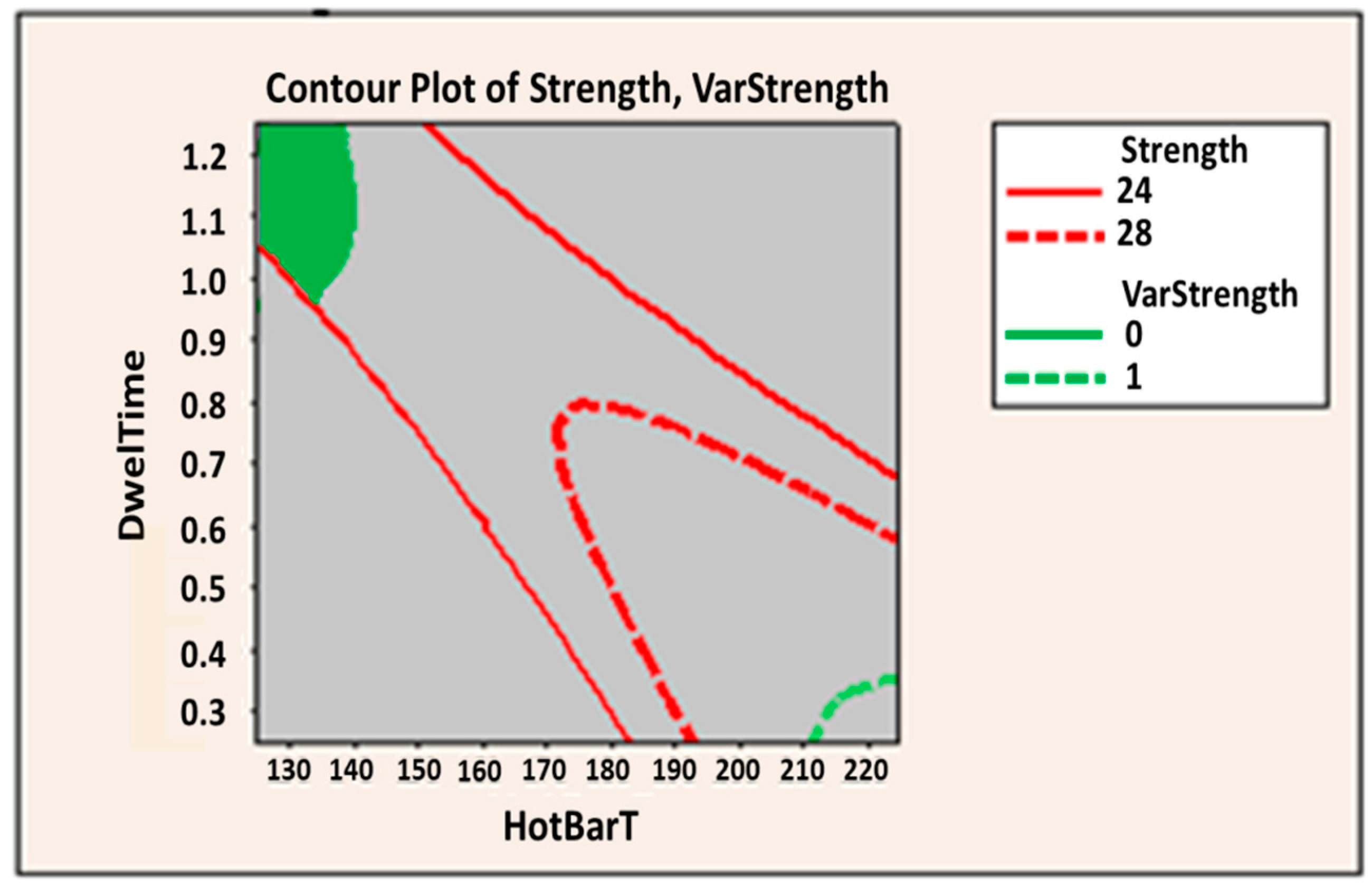
RSM uses different techniques for optimization purposes, such as the contour plots, which allows to visually identify an area of compromise among the response variables. In
Figure 1, it shows as an example for this technique a simultaneous optimization; the green region in the plot is the feasible region that satisfies the criteria for Strength value between 24 and 28 and VarStrength value between 0 and 1.
Other technique is the desirability function analysis popularized by Derring and Suich [
36], where response variables in simultaneous optimization can be maximize, minimize or set to a particular target. Therefore, the first step is to determine the individual desirability index (
di) based on the expected characteristics of the response variable. There are three ways to calculate di; Equation (4) is applied when a particular target is required. Then, the composite desirability (
dG) must be determined through the combination of all individual desirability indexes to form a single value; as seen in Equation (5), this is applied for this purpose. The highest
dG value is the one that determines the optimal parameters and its level combination for response variable optimization. The Minitab software supports both techniques and facilitates the statistical analysis.
where:
3. Materials and Methods
This research was performed with a case study approach in a manufacturing company dedicated to the electronic sector in Tijuana, México. Groat and Wang defined that case study as a methodology that applied different strategies that could help to confirm, challenge or extend a theory [
33,
39,
40]. Base on this, it is considered this method will help to prove the hypothesis described previously.
Two phases are developed for this purpose; first a field research was performed to collect all the information required to build the simulation model. Then, it was considering the steps proposed by Hoover and Perry [
30] to build a discrete event simulation model to represent virtually the real life of logistics process, which considers the following six steps:
Problem statement consists on identifying the entities that are competing for the same resources.
Data collection establishes a diverse range of techniques to perform in this activity. It is necessary to have knowledge of the system to adapt proper techniques. This stage interacts directly with the development, verification and validation of the model. This step was performed with the value stream mapping tool, it was applied as data collection instrument with the following purposes. First to identify and clearly understand the process under study. Second as an instrument for collecting data that are required for the simulation model development, such as: operations, cycle time, material and human resources, entities, resource utilization, attributes, input variables, among others.
Model development, this step considers the construction of the simulation model representing the process under study. It shows how the input variables interact to obtain a specific result within each analyzed scenario. This is the main phase of the simulation methodology, since it interacts with almost all the other phases. In this stage ARENA software was used for modeling and analyzing discrete processes. Based on VSM, the design and construction model was performed with the use of Arena software. This is a friendly software to develop the simulation model logic considering that basic process, advance process and transfer panels are designed based on the symbol used to elaborate flow diagrams, these panels contain the required modules for simulation model development. By last, a model graphic representation was performed, which is useful for model verification purposes.
Verification and validation of the model, this stage focuses on evaluating the consistency of the model, as well as determining the relationship between the model and reality. At this step, if the model does not meet the desired criteria the previous stages would have to be restructured. The validation is executed through a statistical hypothesis test, to determine if the virtual results of the response variables belong to the same population as the actual data of the process,
Experimentation and model optimization consider the statistical analysis to identify the factors’ significance. The optimization method applied in this phase is RSM, which can be defined as an experimental and modeling strategy to find the optimal operation conditions of a process.
Composite central design technique is applied in this step to design all combinations of experiments that can be executed with 2 levels and 3 factors. After this, all experiments are executed in the simulation model elaborated in previous step, in order to observe and collect response variable results under the experimental conditions. Once all information related to response variable is recollected, a statistical analysis is performed for optimization purposes. Finally, Arena and Minitab software were applied as supporting ICT; trough Arena software the virtual model was represented and Minitab software to perform the RSM.
According to the literary review carried out, it was found that there are different investigations in relation to logistic processes, although some authors have used simulation models in their investigations. These do not focus on the systematic optimization of logistics costs, so: Ugarte [
4] focused on evaluating environmental impacts in logistics processes; Guo et al. [
22] explored if there is an adequate allocation of resources between production and logistics systems; Papoutsis [
23] investigated the key factors affecting retail logistics solutions in total costs and sustainability performance; Tamás [
26] conducted research to improve the programming of batches that will occur in intermittent production systems.
On the other hand, there are researchers who have used other methods to evaluate alternatives to support decision making in logistic processes, such as those carried out by: Holzapfel et al. [
27] apply deterministic methods (Mixed Integer Programming) for the optimal allocation of inventory in the distribution centers; and Vidal et al. [
28] use the analytical hierarchy process for the design of distribution centers in which the variables under study are: distribution strategy, internal activities and the characteristics of the distribution operations; which are not evaluated with purely quantitative methods.
Finally, it was identified that there are researches that focus on the optimization of the logistic cost, however they do not use stochastic methods that represent in a more adequate way the real situation of the process, it is so: Ji [
24] carries out the research with the purpose to minimize the cost of inventory and the cost of transportation without considering the implications of the cost that can be generated by non-compliance with deliveries to customers; and Noroozi et al. [
29] did a similar work in relation to the analysis of the response variables under study in the present investigation, however the method applied was linear programming (deterministic method). In this respect, the contribution of this document is the application of stochastic methods, which represent in a better way the real-life processes through integration of probabilistic techniques. Additionally, with the stochastic methods the optimization for objective function can be focused to: maximize, minimize or identify nominal values for response variables; while deterministic methods are normally used to maximize or minimize the objective function.
4. Case Study
This section focuses on presents the application of the case study for the logistic process optimization of a television manufacturing company that supply finished good from two distribution centers to their customers.
4.1. Problem Statement
For this case study, a manufacturing company was chosen. The company relies on two service providers to execute the logistics process in Mexico. The company’s strategy is to allocate up to 30% of production to the logistics provider located in Tijuana for the distribution of FG to the retail customer located in Culiacan, Mexico; so, the remaining 70% is shipped to a distribution center located in the city of Mexico to perform the FG distribution from that point to their other customers located in Guadalajara, Monterrey, Mexico City and Veracruz. Therefore, the aim of this case study is to identify if increasing the volume assigned to the logistics service provider located in Tijuana and doing the distribution of FG from this point, the logistics process cost is improved, using stochastics tools for this purpose.
4.2. Data Collection and Analysis
The first step is to determine the products (FG) to be evaluated, for this purpose the two highest runner products were selected, which are two models of 40″ TV’s. Then the operations involved to perform the logistics process were identified, among which are the storage, transportation and inventory level; that according to studies conducted represent between 85% and 90% of the logistics cost [
1]. Finally, we collect the FG inventory target in days that are defined by the manufacturer and the transportation transit time committed by the carriers and the information necessary to develop the simulation model. The second step is to identify the different elements that should be considered in the simulation model, which are:
Entities. Finished Goods (Containers/TVs), as well as customers located in Mexico City, Culiacan, Monterrey, Guadalajara y Veracruz.
Variables. Two types of variables are considered. Cost to perform the logistics process, which is considered the output variable to be analyzed. Also, the input variables that are: FG allocation by supplier, Inventory level and on time delivery performance.
Resources. In order to perform the logistics process, the resources considered are shown in
Table 1.
Statistics. This activity is considered to accumulate the statistics of the response variable, which is the cost of logistics process.
4.3. Simulation Model Design
Once step 4.2 is completed, the simulation model design needs to be performed based on the operations defined for the logistics process, as well as the interactions of entities, variables and resources. The representation of simulation model is shown in
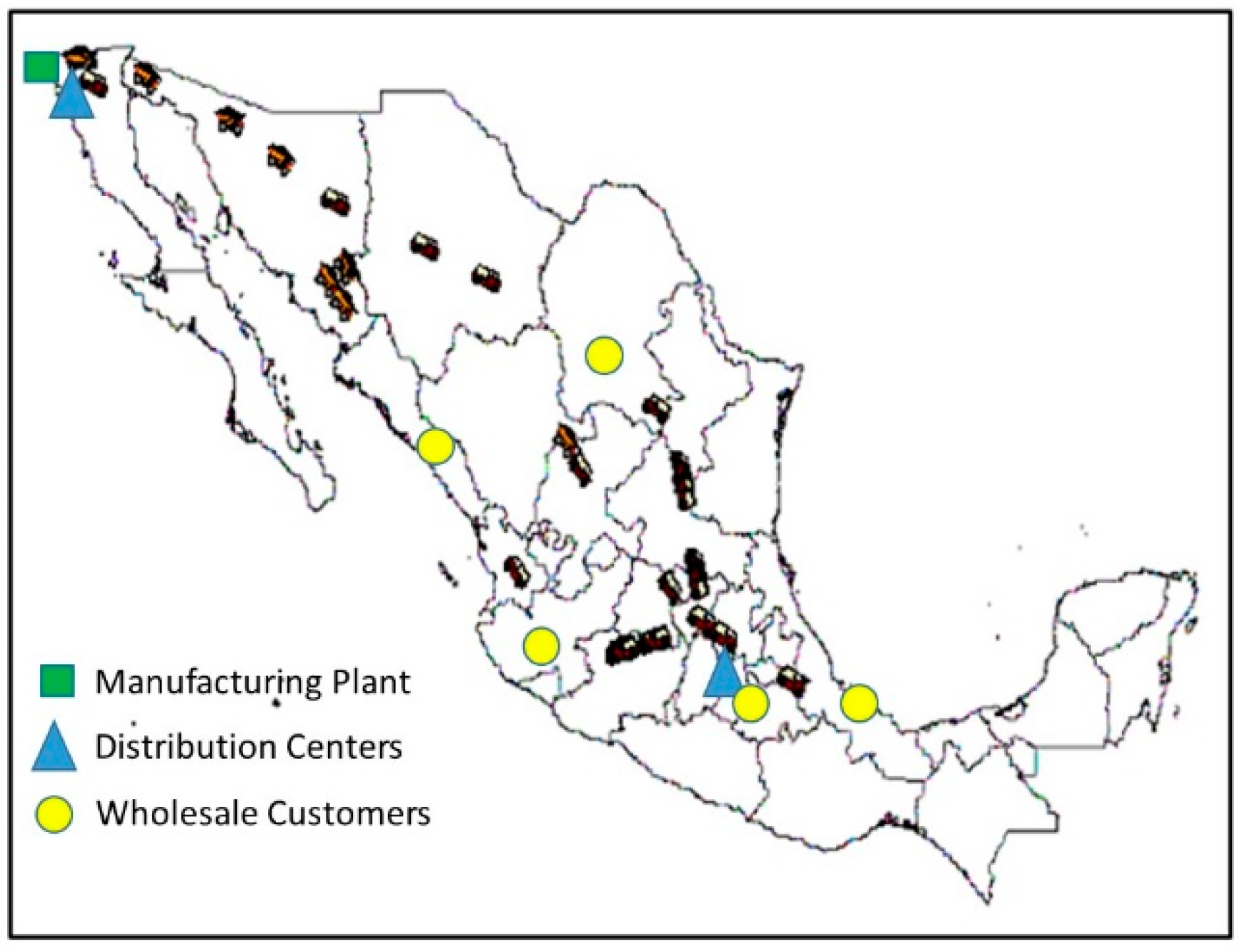
Figure 2; the model assumes a constant output of a TV’s every minute from the production line. Also, that product is shipped from manufacturing plant by truck to two distribution centers, located in Tijuana and Mexico City to be storage before it is shipped to the wholesale customer; allocation for each customer is 30% for the Tijuana logistics service supplier and 70% to the logistics service supplier located in Mexico City. Finally, the model considers some failure such as the on-time deliveries to customers, which has an economic penalty.
4.4. Verification and Validation of the Model
At this phase, verification is done by running the model to confirm that the different operations are executed without any problem; after that validation, a comparison of the results is issued by the model and it is made in terms of the cost of the logistics process. Hence, the result was a cost of $ 11,735,575 per 150 shipments evaluated.
4.5. Experimentation and Model Optimization
Three factors were considered and tested in two levels each one in the simulation model as follow: product allocation (PA), considering 30% low level and 70% as high level for Tijuana Distribution Center (TDC); inventory level (IL), tested at 1 week in low level and 2 weeks in high level and on time delivery (OTD), 80% low level and 95% high level. The central composite technique (CCD) of RSM is going to be applied with face centered, four central points and 0.05 significance level (α). This activity is performed with Minitab Software and the design considers 18 experimental runs with different combinations of each level.
Each of the 18 experimental runs were executed in the simulation model designed in
Section 4.3 to find out the cost of logistics process under the different scenarios, all the information is collected in order to execute the statistical analysis.
Table 2 shows the 18 experimental runs and results obtained with the DCC; coded units −1, 0, 1 in the design indicates: Pt type −1 experiment is executed with axial points, Pt type 0 executed with central points and Pt type 1 executed with factorial points; Blocks 1 specify DCC is performed considering only one block; and −1, 0, 1, for variables PA, IL and OTD indicates level to test in the DCC, “−1” represents the low level value, “0” nominal level value and “1” high level value.
Once, the LC results of each experiment executed in the DCC are attained, the information is expressed in equations of matrix form to determine the value for each coefficient applying Equation (6).
where:
Software Minitab
®, was used to calculate the value for each coefficient included in the empirical mathematical model represented by the Equation (7), this needs to be validating to determine if it is a good estimator for the response variable. This model is represented by a regression model with a second order equation. The following concepts are analyzed (where X
1 = PA, X
2 = IL, X
3 = OTD):
Coefficient of determination analysis (R2adj). This indicator shows as a result 96.89%, which indicates that the factors are statistically significant to the result (output variable), because those factors explain the 96.89% of the variability by the fitted model. Base on this information, the empirical mathematical model represented by the equation 2 needs to be validated to determine if it is a good estimator for the response variable.
Analysis of variance (ANOVA) is applied to ensure the significance of the regression model at 5% significance level (α). Based on the ANOVA results shown in the
Table 3, it can be concluded that the regression is statistically significant at a F-value of 59.89 and
p-values of 0.00; principal effects (PA, IL and OTD) and quadratic effects also are significant for the response variable (logistics cost) since
p-value is less than α-value. As well as, model fit the data since the
p-value for lack of fit is greater than α-value.
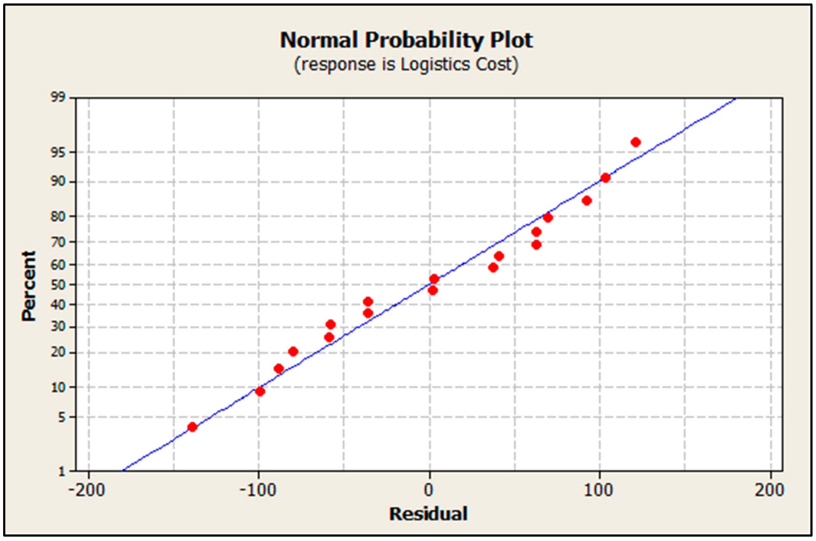
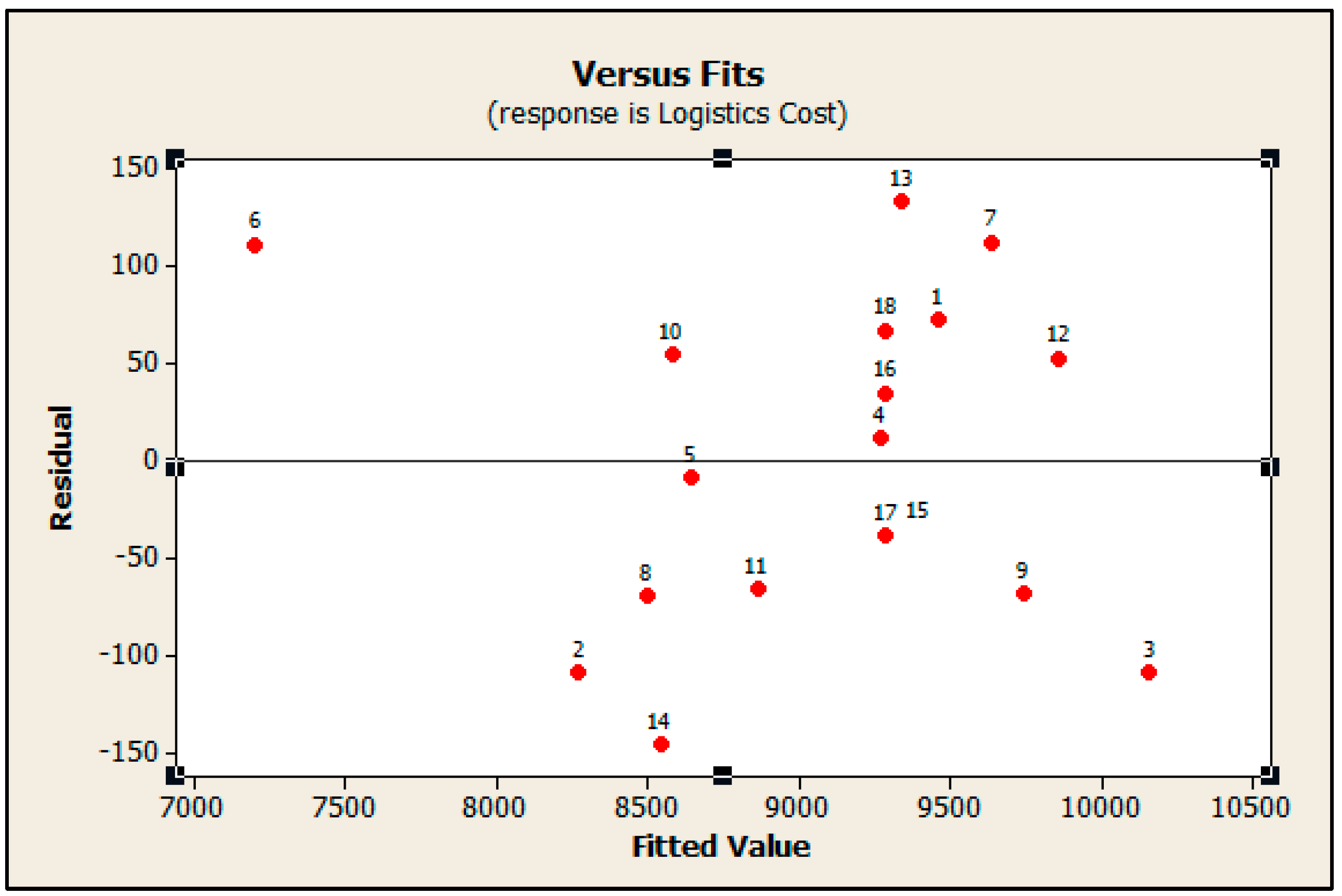
Residuals analysis is performed to determine how good the fitted model is. This analysis helps to determine if the ordinary least square assumptions are met to produce unbiased coefficient estimates with minimum variance. The residual Normal Probability Plot is in
Figure 3, the points on the plot form a straight line, therefore it can be confirmed residuals are normally distributed. In
Figure 4 shows residuals are distributed randomly and with similar distance on both sides of zero, therefore there are no outlier points, as well as, the plot confirms the equal variance assumption on the model. Therefore, it can be concluded that data transformation is not required.
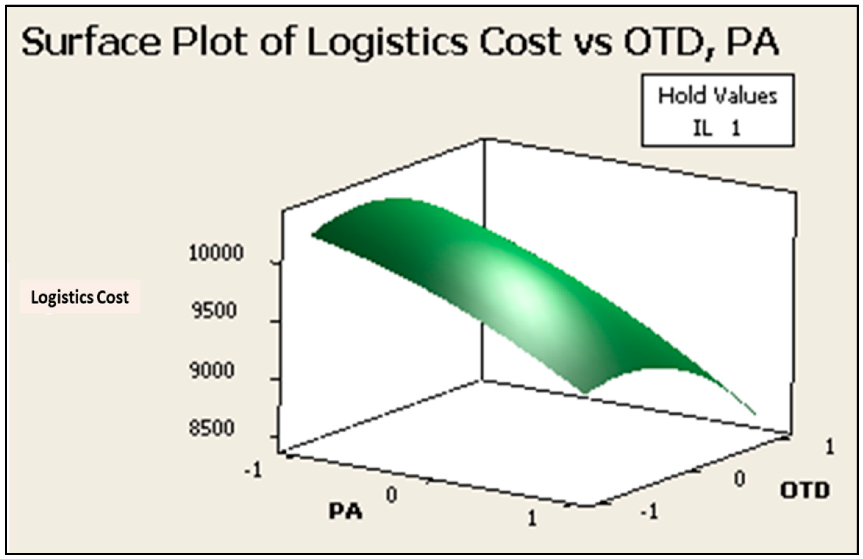
The empirical mathematical model can be evaluated through the Response Surface and Contour Plots; which are visual tools for interpreting the result of the CCD. The Surface Plot in
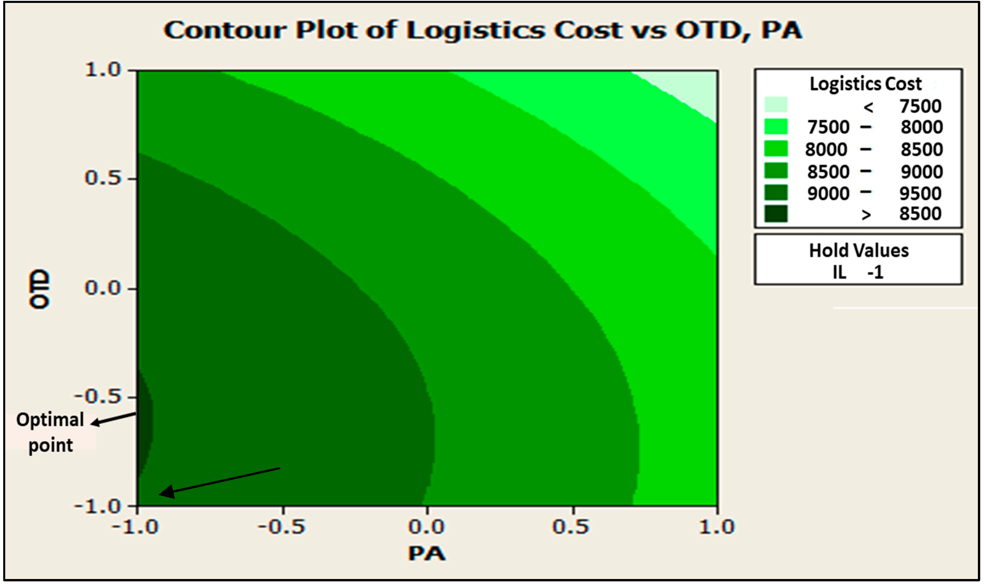
Figure 5 indicates the CCD model reaches a maximum logistics cost when PA is at low level as well as OTD, keeping blocked the IL at high level. In
Figure 6, the contour plot is reflecting that the stationary point (Maximum) for the model is out of the experimental region, therefore a canonical analysis can be performed in order to determine the optimal point of the model. In this step, it can be validated that current logistics operations are according to the results of the model.
Once the second order empirical mathematical model has been evaluated and confirmed, it is appropriate to define optimal points. Canonical analysis is performed applying the Equation (8), in order to define the stationary points.
where:
where
xs is any point in the region of process operability in coded units; vector
b includes the coefficients of the linear part of the model and the matrix
B includes the coefficients of quadratic terms and interactions pure. Then stationary points are the solution of Equation (9).
The
xs,
b and
B matrices in Equation (8) were arranged by Equation (6) to get Equation (10) as follows:
The solution for Equation (9) defines the optimum values for the model in coded units, such values are −2.7, −1.6 and 0.5 for PA, IL and OTD respectively. This result shows clearly that stationary point is out of the experimental region. Applying the Equation (11), where
ZH and
ZL are the high and low levels values for independent variables in original units, as well as
Xi is the value in coded units defined in Equation (5), the optimum values can be decoded in order to get original units, getting the value for PA equal to 0%, which means logistics operations needs to be managed by the logistics service supplier located at Mexico City, IL is going to keep at 0.67 and OTD at 84%.
Based on the information obtained in this step, it can be concluded that parameters determined with the mathematical model reflect the traditional operation in which the logistics process is performed by a supplier closer to the customers, in this case in Mexico City, at the highest operational cost. Since the goal of this research project is to find alternatives that optimize the logistics cost, we will proceed to evaluate the empirical mathematical model to determine if there is a better regression equation to estimate the parameters of optimizing the logistics costs.
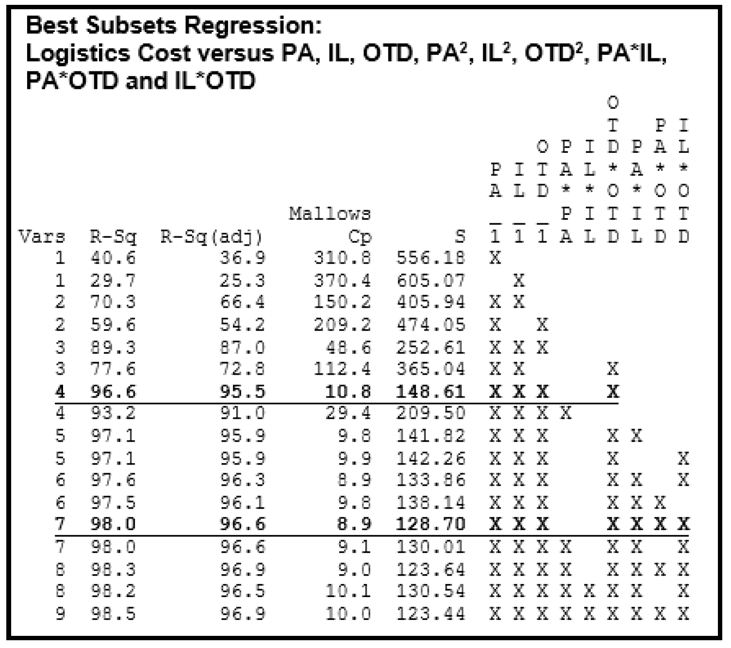
A subsets regression technique was applied to evaluate the empirical mathematical model; this technique attempts to identify groups of predictors for further analysis. Ideally, the smallest subset that fulfills certain statistical criteria such as highest coefficient of determination adjusted (R2adj.), lowest Mallow’s Cp and Mean Square Error (S) should be selected. Because, this subset of predictors may estimate the regression coefficients and predict future responses with smaller variance than the full model using all predictors.
This process was performed with the support of Minitab software,
Figure 7 shows that a seven predictors subset is the one that fulfill the statistical criteria mentioned previously; however, there is a smaller subset with four predictors with similar statistical criteria, therefore a further analysis was done with both subgroups.
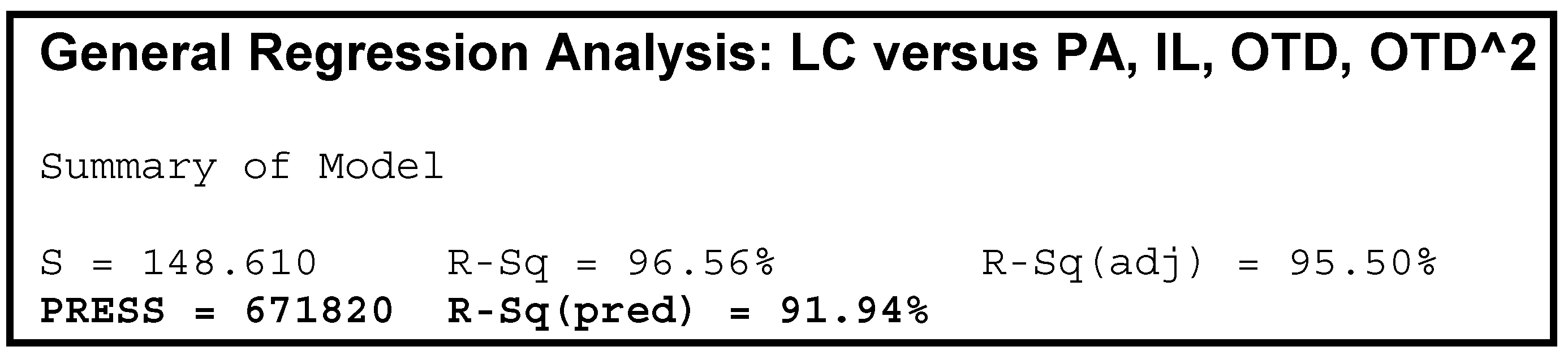
Finding that four predictors subset is a better estimator since Predicted Residual Square Sum value is the smaller (671820) as show in
Figure 8. Therefore, the coefficient of determination to predict values will be the highest (91.94%) of the all subgroup. As a conclusion Equation (12) is the best regression equation to predicted values.
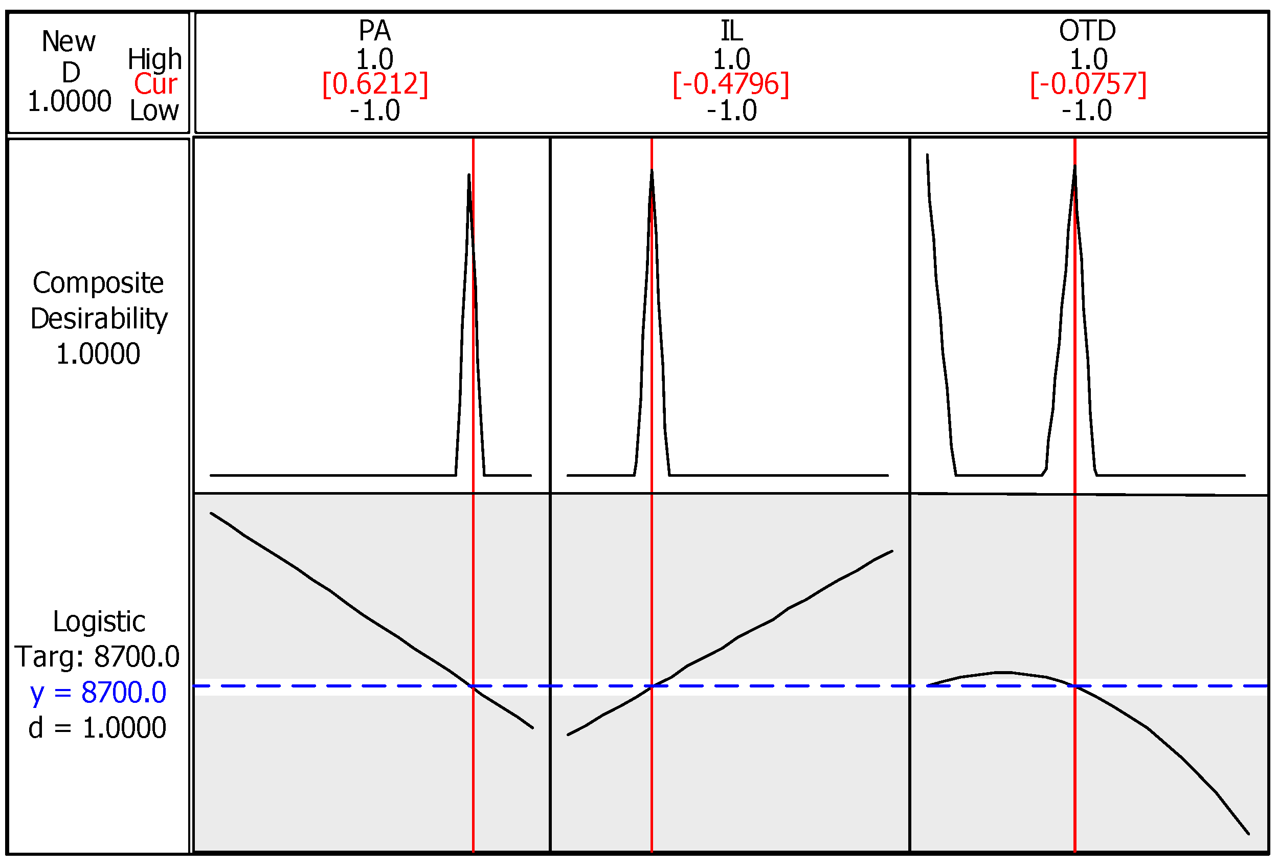
Once the validation of the model is completed, the model can be optimized. This process is going to define the parameters of the independent variables (PA, IL and OTD) which provide an optimal operation condition to achieve a particular objective for the logistics process cost. As Assumption for the model is to improve the logistics cost by 15% ± 2%. Therefore, the cost must be between $8525 and $8875 and a target of $8700 (thousands of USD). Based on this information we utilized the Minitab response optimizer module to define the optimal operation condition.
The optimum parameters in coded units for independent variables are showed in
Figure 9 highlighted in red. Indicating that PA needs to be set up at 0.6212, which represents increasing the business with the logistics supplier located in Tijuana from 30% to 60%, the IL level parameter is—0.4798 which represent in decoded units 1.2 weeks and OTD is—0.0757, which is 87% in decode units.
5. Results
The purpose in this research project was achieved, since a strategy for TLC improvement was defined with the application of stochastics tools. As a result of this research, different alternatives were evaluated to define a mathematical model for optimization purpose; therefore, this project included:
Design a simulation model to represent in a virtual way, the real life of a complex process, as described in
Section 4.3 and
Section 4.4. As well as, it is defined in
Section 4.5, the application of a statistical technique was performed to evaluate 18 different alternatives indicating how process can be developed, the results for this activity defined the logistics cost for each alternative Lastly, it was performed a statistical analysis to define an empirical mathematical model represented for regression Equation (10), that helps us to make estimations for a particular objective of the logistics process cost.
The application of the empirical model is described on the
Table 4; where, the parameters for PA, IL and OTD were defined in order to achieve a cost improvement of 5%, 10% and 15%. As an outcome, the model describes that as much as the product allocation is increased for the DC located in Tijuana, the logistic cost is improved proportionally. Also, distribution activity can be managed with fewer inventories without affecting customer delivery performance, since this indicator is increased based on the simulation model evaluated.
6. Conclusions
Based on the hypothesis statement posed in
Section 1, it can be concluded that stochastics tools can be used to define strategies to improve logistic cost without affecting customer service. For this purpose, this research was validated with a case study in a logistics process where the variables Product Allocation PA, Inventory Level IL and On Time Delivery OTD were evaluated. The results states that strategy needs to consider increase PA and reduce IL to improve cost, at this same time these changes are going to help to improve the OTD.
As it was stated in the introduction, two of the main contributor to the logistics cost are the transportation and inventory management; both elements were considered, showing in the results that PA needs to be increased to the DC located in Tijuana, which automatically reduces the transportation activity since the product will travel less distance to be delivered to the customer; in the other hand, shipping directly from Tijuana DC allows to has a leaner logistics process having as a result the FG inventory reduction. Both activities help to increase the on-time delivery, which is one of the main key performance indicators related to the customer service.
Through this study, we demonstrate that integrated simulation-based optimization is a well-founded decision-making tool. Information technologies facilitate the application of complex techniques such as simulation and applied statistics quickly and efficiently by middle and/or top management with the application of predefined models. As consequence, better business strategies related to the logistics process are taken by the decision makers.
Finally, the development of this research can corroborate the importance of stochastic tools application for the optimization purpose in a transactional process (support activities for manufacturing process). The optimization steps have shown that the applied model helps to represent in a virtual way a complex process that hardly can execute the experiments activity in real time. As well as, this research could be a good practice to disclose in academia environment.
Author Contributions
Conceptualization, J.G.R. and H.H.R.; methodology, J.G.R. and A.R.V.; validation, J.G.R.; formal analysis, K.C.A.S. and A.R.V.; investigation, J.G.R.; resources, K.C.A.S. and T.C.G.; writing—original draft preparation, J.G.R.; writing—review and editing, K.C.A.S. and A.R.V.; supervision, K.C.A.S. and A.R.V.; project administration, J.G.R. and H.H.R.
Funding
This research received no external funding.
Acknowledgments
We would like to thank CONACYT, PRODEP, the National Technological Institute of Mexico (TecNM) and the Autonomous University of Baja California for their support in carrying out and publishing this project.
Conflicts of Interest
The authors declare no conflict of interest.
References
- Arayapan, K.; Warunyuwong, P. Logistics Optimization: Application of Optimization Modeling in Inbound Logistics; Malardalen University: Västerås, Sweden, 2009. [Google Scholar]
- Lee, H.L. Effective Inventory and Service Management through Product and Process Redesign. Oper. Res. 1996, 44, 151–159. [Google Scholar] [CrossRef]
- Migdadi, M.M.; Zaid, M.K.S.A.; Yousif, M.; Ra’d, A. An empirical examination of collaborative knowledge management practices and organisational performance: The mediating roles of supply chain integration and knowledge quality. Int. J. Bus. Excell. 2018, 14, 180–211. [Google Scholar] [CrossRef]
- Ugarte, G.M.; Golden, J.S.; Dooley, K.J. Lean versus green: The impact of lean logistics on greenhouse gas emissions in consumer goods supply chains. J. Purch. Supply Manag. 2016, 22, 98–109. [Google Scholar] [CrossRef]
- Rantasila, K.; Ojala, L. Measurement of National-Level Logistics Costs and Performance; OCDE: Paris, France, 2012. [Google Scholar]
- OCDE; Banco de Desarrollo de América Latina. CEPAL Perspectivas Económicas de América Latina 2017; OCDE: Paris, France, 2017. [Google Scholar]
- Straubea, F.; Durach, C.F.; Phungb, J. Developing and applying a supplier selection model to account for supplier...: Recursos Informativos UABC. Supply Chain Forum Int. J. 2016, 17, 68–77. [Google Scholar] [CrossRef]
- Safizadeh, M.H. Optimization in simulation: Current issues and the future outlook. Nav. Res. Logist. 1990, 37, 807–825. [Google Scholar] [CrossRef]
- PRO MEXICO. Trade and Investment. 2018. Available online: http://negocios.promexico.gob.mx/english/12-2009/art03.html (accessed on 22 November 2018).
- Brito, J. Situación Actual y Prospectiva de la Industria de Televisores en Tijuana; Ciudad Universitaria: Mexico City, Mexico, 2013. [Google Scholar]
- A Look Back at IFA 2014—Samsung Global Newsroom. 2014. Available online: https://news.samsung.com/global/a-look-back-at-ifa-2014 (accessed on 22 November 2018).
- Li, Y. Analysis of logistics lean management based on modern manufacturing enterprises. J. Adv. Oxid. Technol. 2018, 21. [Google Scholar] [CrossRef]
- Hammadi, S.; Herrou, B. Energetic equipment maintenance logistics: Towards a lean approach. J. Eng. Appl. Sci. 2018, 13, 4188–4192. [Google Scholar] [CrossRef]
- Oey, E.; Nofrimurti, M. Lean implementation in traditional distributor warehouse—A case study in an FMCG company in Indonesia. Int. J. Process. Manag. Benchmark. 2018, 8, 1–15. [Google Scholar] [CrossRef]
- Buonamico, N.; Muller, L.; Camargo, M. A new fuzzy logic-based metric to measure lean warehousing performance. Supply Chain Forum 2017, 18, 96–111. [Google Scholar] [CrossRef]
- Sumantri, Y. Lean logistics implementation level in Small and Medium Enterprises (SMES) sector. J. Eng. Appl. Sci. 2017, 12, 195–198. [Google Scholar] [CrossRef]
- Daneshjo, N.; Dudaš Pajerská, E.; Klimek, M.; Danishjoo, E. Software Support for Optimizing Layout Solution in Lean Production. TEM J. 2018, 7, 33–40. [Google Scholar] [CrossRef]
- Wang, X. Optimization study based on lean logistics in manufacturing enterprises. In Proceedings of China Modern Logistics Engineering; Springer: Berlin, Germany, 2015. [Google Scholar]
- Zhang, A.; Luo, W.; Shi, Y.; Chia, S.T.; Sim, Z.H.X. Lean and Six Sigma in logistics: A pilot survey study in Singapore. Int. J. Oper. Prod. Manag. 2016, 36, 1625–1643. [Google Scholar] [CrossRef]
- Le, N.T. Collaborative Direct to Store Distribution: The Consumer Packaged Goods Network of the Future; Massachusetts Institute of Technology: Cambridge, MA, USA, 2011. [Google Scholar]
- Rossini, M.; Portioli, A. Supply chain planning: A quantitative comparison between Lean and Info-Sharing models Supply chain planning: A quantitative comparison between Lean and Info-Sharing models. Prod. Manuf. Res. 2018, 6, 264–283. [Google Scholar] [CrossRef]
- Guo, Z.; Zhang, Y.; Zhao, X.; Song, X. A Timed Colored Petri Net Simulation-Based Self-Adaptive Collaboration Method for Production-Logistics Systems. Appl. Sci. 2017, 7, 235. [Google Scholar] [CrossRef]
- Papoutsis, K.; Dewulf, W.; Vanelslander, T.; Nathanail, E. Sustainability assessment of retail logistics solutions using external costs analysis: A case-study for the city of Antwerp. Eur. Transp. Res. Rev. 2018, 10, 34. [Google Scholar] [CrossRef]
- Ji, M.; Fang, J.; Zhang, W.; Liao, L.; Cheng, T.C.E.; Tan, Y. Logistics scheduling to minimize the sum of total weighted inventory cost and transport cost. Comput. Ind. Eng. 2018, 120, 206–215. [Google Scholar] [CrossRef]
- Ndhaief, N.; Bistorin, O.; Rezg, N. An Improved Distribution Policy with a Maintenance Aspect for an Urban Logistic Problem. Appl. Sci. 2017, 7, 703. [Google Scholar] [CrossRef]
- Tamás, P. Decision Support Simulation Method for Process Improvement of Intermittent Production Systems. Appl. Sci. 2017, 7, 950. [Google Scholar] [CrossRef]
- Holzapfel, A.; Kuhn, H.; Sternbeck, M.G. Product allocation to different types of distribution center in retail logistics networks. Eur. J. Oper. Res. 2018, 264, 948–966. [Google Scholar] [CrossRef]
- Geraldo Vidal Vieira, J.; Ramos Toso, M.; Eduardo Azevedo Ramos da Silva, J.; Cristina Cabral Ribeiro, P. An AHP-based framework for logistics operations in distribution centres. Int. J. Prod. Econ. 2017, 187, 246–259. [Google Scholar] [CrossRef]
- Noroozi, A.; Mazdeh, M.M.; Heydari, M.; Rasti-Barzoki, M. Coordinating order acceptance and integrated production-distribution scheduling with batch delivery considering Third Party Logistics distribution. J. Manuf. Syst. 2018, 46, 29–45. [Google Scholar] [CrossRef]
- Hoover, S.; Perry, R. Simulation: A Problem-Solving Approach; Prentice Hall: Upper Saddle River, NJ, USA, 1989. [Google Scholar]
- Kumar Shukla, R.; Garg, D.; Agarwal, A. Understanding of Supply Chain: A Literature Review. Int. J. Eng. Sci. Technol. 2011, 3, 2059–2072. [Google Scholar]
- David, W.; Retired, R.P.S.; Zupick, N.B. Simulation with Arena, 6th ed.; McGraw-Hill Education: New York, NY, USA, 2015. [Google Scholar]
- Aldemir, A.; Hapoglu, H.; Hapoğlu, H.; Alpbaz, M. Optimization of Generalized Predictive Control (GPC) Tuning Parameters By Response Surface Methodology (RSM). Int. J. Control Autom. 2015, 8, 393–408. [Google Scholar] [CrossRef]
- Izadi, A.; Kimiagari, A.M. Distribution network design under demand uncertainty using genetic algorithm and Monte Carlo simulation approach: A case study in pharmaceutical industry. J. Ind. Eng. Int. 2014, 10, 50. [Google Scholar] [CrossRef]
- Chackelson, C.; Errasti, A.; Ciprés, D.; Lahoz, F. Evaluating order picking performance trade-offs by configuring main operating strategies in a retail distributor: A Design of Experiments approach. Int. J. Prod. Res. 2013, 51, 6097–6109. [Google Scholar] [CrossRef]
- Carson, Y.; Maria, A. Simulation optimization: Methods and applications. In Proceedings of the 1997 Winter Simulation Conference; Andradottir, S., Healy, K.J., Withers, D.H., Nelson, B.L., Eds.; Renaissance Waverly Hotel: Atlanta, GA, USA, 1997; pp. 118–126. [Google Scholar]
- Ramanujam, R.; Raju, R.; Muthukrishnan, N. Taguchi Multi-machining Characteristics Optimization in Turning of Al-15%SiCp Composites using Desirability Function Analysis. J. Stud. Manuf. 2010, 1, 120–125. [Google Scholar]
- González, J.; Híjar, H.; Sánchez-Leal, J.; Hernández, D.E. Simulation and Surface Response Methodology for Simultaneous Optimization of Response Variables: Case Study in a Warehousing Process. In Proceedings of the AHFE 2017 International Conferences on Human Factors in Management and Leadership, and Business Management and Society, Los Angeles, CA, USA, 17–21 July 2017; pp. 426–437. [Google Scholar]
- Wang, D.; Groat, L.N. Architectural Research Methods; Wiley: Hoboken, NJ, USA, 2013. [Google Scholar]
- Yin, R.K. Case Study Research Design and Methods, 2nd ed.; SAGE Publications: Thousand Oaks, CA, USA, 2003. [Google Scholar]
© 2018 by the authors. Licensee MDPI, Basel, Switzerland. This article is an open access article distributed under the terms and conditions of the Creative Commons Attribution (CC BY) license (http://creativecommons.org/licenses/by/4.0/).


 ,
, 


