A Robust Maximum Power Point Tracking Control Method for a PEM Fuel Cell Power System


1
Departament of Automatic Control and System Engineering, Engineering School, University of the Basque Country UPV/EHU, Nieves Cano 12, 1006 Vitoria, Spain
2
Research Unit of Photovoltaic, Wind and Geothermal Systems SPEG/UR11ES82, National Engineering School of Gabes, University of Gabes, Omar Ibn-Elkhattab, Zrig, 6029 Gabès, Tunisia
*
Author to whom correspondence should be addressed.
Appl. Sci. 2018, 8(12), 2449; https://doi.org/10.3390/app8122449
Submission received: 2 November 2018
/
Revised: 23 November 2018
/
Accepted: 29 November 2018
/
Published: 1 December 2018
(This article belongs to the Special Issue Renewable Fuels)
Abstract
:Taking into account the limited capability of proton exchange membrane fuel cells (PEMFCs) to produce energy, it is mandatory to provide solutions, in which an efficient power produced by PEMFCs can be attained. The maximum power point tracker (MPPT) plays a considerable role in the performance improvement of the PEMFCs. Conventional MPPT algorithms showed good performances due to their simplicity and easy implementation. However, oscillations around the maximum power point and inefficiency in the case of rapid change in operating conditions are their main drawbacks. To this end, a new MPPT scheme based on a current reference estimator is presented. The main goal of this work is to keep the PEMFCs functioning at an efficient power point. This goal is achieved using the backstepping technique, which drives the DC–DC boost converter inserted between the PEMFC and the load. The stability of the proposed algorithm is demonstrated by means of Lyapunov analysis. To verify the ability of the proposed method, an extensive simulation test is executed in a Matlab–Simulink environment. Compared with the well-known proportional–integral (PI) controller, results indicate that the proposed backstepping technique offers rapid and adequate converging to the operating power point.
1. Introduction
The entire world lives in a great crisis of energy and environment. This fact behooves many researchers to look for efficient and clean energy sources. Producing clean energy can reduce the pollution caused by carbon dioxide emissions (CO). Therefore, several countries are installing solar and wind power plants to decrease these CO emissions [1,2]. One drawback of these energies is their dependency on weather conditions. Solar energy depends on the sun, and the wind tends to blow intermittently. Furthermore, storing surplus energy produced during times of abundance is a hard task. Fuel cells are thus one of the most important alternative sources of clean renewable energy. Moreover, due to their effectiveness and reliability, fuel cells have become one of the most promising power generators. They can provide a continuous power supply throughout all seasons as long as fuel is provided. The most preferable fuel is hydrogen. Hydrogen is a clean renewable energy source. A PEM fuel cell (PEMFC) is a fuel cell that combines hydrogen and oxygen to produce energy. It is characterized by several advantages including a quiet operation, robustness and high efficiency, and produced energy with zero levels of pollutant gases, which is why it is touted as environmentally friendly [3,4]. In many applications, fuel cell generators are used in conjunction with power converters that provide an efficient power conversion from the cell stack to the load and that offer a regulated output voltage [5]. Since the PEMFC generates a low output voltage, a high step-up power converter is used to boost and regulate the fuel cell voltage in order to make the PEMFCs operate at the optimal power point as well as providing an applicable direct current (DC) power source. On the other hand, the PEMFC output characteristics are influenced by changes in several parameters, such as the cell temperature, the oxygen and hydrogen partial pressure, and the load demands [6]. Therefore, an MPPT algorithm must be established for optimal and proper operation.
In the literature, a great number of classical MPPT methods have been reported [7,8,9,10,11,12,13,14,15,16,17,18,19,20,21,22,23,24,25,26,27,28,29,30,31,32,33,34]. However, the most commonly used are fractional short or open-circuit (FSC, FOC) [7,8], perturb and observe (P&O) [9,10,11], voltage- and current-based MPPT [12], incremental conductance (Inc-Cond) [13,14,15], extremum seeking control (ESC) [16,17,18,19], sliding mode control (SMC) [20,21,22,23], current sweep (CS) [24], and fuzzy logic control (FLC) [25,26,27,28,29,30]. Smart and advanced computing techniques such as eagle strategy control (ESC), particle swarm optimization (PSO), neural network control (NNC), and genetic algorithms (GAs) have also been commonly used in the last few years [35,36,37,38,39,40,41,42]. Each method of these existing algorithms is characterized by its complexity in hardware implementation, convergence speed, the sensors required, the sensed parameters, and the cost. Despite the simplicity of the fractional open-circuit voltage and current, shown in [7,8], a low efficiency and accuracy remain their main drawbacks. The P&O and Inc-Cond techniques are widely used as conventional algorithms with certain features and drawbacks. The P&O algorithm has the drawback of oscillations around the operating power point, which yields a loss of a considerable amount of power [10]. Moreover, the response of the P&O technique is slow-moving under rapid changes in operating conditions. Many other algorithms such as the variable step-size incremental resistance algorithm (VSIR) and the gradient descent algorithm (GRD) may overcome the drawbacks of these well known P&O and Inc-Cond methods [13,14,43]. Several advantages of ripple correlation control (RCC) over P&O are discussed in [44,45,46]. According to [47], despite its hardware implementation complexity, the sliding mode control technique shows high accuracy compared with conventional methods. However, in the presence of large load disturbance and uncertainties, its switching gain becomes higher, which leads to the production of a large amplitude of chattering. The computing techniques yield a high tracking efficiency, but the whole system cost becomes too expensive.
The backstepping technique has recently attracted considerable attention. It is a recursive design methodology developed in 1990 by P. V. Kokotovic and his coauthors for designing stabilizing controls. It has become an important robust algorithm due to its ability to control chaos and its flexibility in the construction of control law. It is commonly used for numerous applications, especially nonlinear uncertain systems (e.g., PEMFC power systems) [48,49,50,51,52,53,54,55,56,57,58,59]. In [48], it is used for a smart grid-connected distributed photovoltaic system. It is designed to track the PV array maximum power point in order to power up the telecom towers. Similarly, it is also proposed in [49,50] to track the MPP reference voltage, which is generated using the incremental conductance algorithm. In [51], it is used to adapt the turbine speed at its maximum generator speed value. However, pitch control and proportional–integral (PI) regulators are used to determine the optimal specific speed at which the turbine generates its maximum power. In [55], it is proposed for a PV water desalination system. It dissipates the maximum produced power in a resistive load to generate heat, which is then used for the desalination process. In [59], it is proposed to reduce the steady state error, which degrades the efficiency of the MPPT controller. The authors used a regression plane to determine the reference voltage, which corresponds to the peak power.The current paper proposes a new MPPT method based on a backstepping algorithm to keep the system functioning at its optimal power point. The main feature of this method is its simplicity, robustness, and high tracking performance, confirmed by the obtained results. The global system including the fuel cell, the DC–DC converter, and the controllers are presented, modeled, identified, and then tested under a Matlab–Simulink environment. The obtained simulation results are analyzed and discussed. Finally, some conclusions are made and future works are suggested.
2. PEM Fuel Cell
As shown in Figure 1, a PEMFC is composed of a catalyst layer (CL), a gas diffusion layer (GDL), and an electrolyte membrane. Each of these components is fabricated individually and then pressed to each other at high pressures and temperatures. The CL and GDL are placed on both anode and cathode sides. The electrolyte membrane permits only the appropriate ions (protons) to migrate toward the cathode. The PEMFC is supplied by pressurized hydrogen (H) and oxygen (O) as a fuel and generates electricity, water, and heat. The hydrogen atoms (H) enter the PEMFC at the anode side, where the CL divides them into protons (H) and electrons (). The protons flow to the cathode via the electrolyte membrane, while the electrons flow through the external circuit to provide electric energy along the way. The oxygen atoms (O) enter the PEMFC at the cathode side and react with electrons returning from the external circuit and with protons that have traveled through the membrane to produce water and heat [60].
The electrochemical reactions occurring on the electrodes can be described in Equations (1)–(3). The first and the second equations show the anode and the cathode side reactions, respectively, and the third equation shows the overall electrochemical reaction [61].
The energy of Equation (3) is called the enthalpy of formation . It can be divided into two kinds of energies: the first one is the thermal energy represented by the specific entropy multiplied by the temperature T, and the second is the useful work . is also called the negative thermodynamic potential (or Gibbs free energy). Therefore, the total energy as given in [62] is
can be extracted as an electric work, defined by the charge Q across the potential E. Q is the number of electrons (released from the anode), multiplied by the Faraday constant F. Therefore, the useful work can be calculated by Equation (5):
Using Equations (4) and (5), the PEMFC potential can be calculated by Equation (6), where , , and are negative due to the exothermic reaction (yields energy).
The values of the useful work , which is given in Equation (5), also depend on the reactants. Therefore, it can also be calculated using Equation (7):
where R is a universal constant, and are, respectively, the partial pressure of hydrogen and oxygen, and is at the standard condition. Therefore, by placing Equation (7) into Equation (6), the PEMFC potential can be given as
at the standard condition ( = 25 C, ). The term is equal to V. It varies with the temperature according to the following expression:
However, in practice as shown in Figure 2, the potential of the PEMFC is significantly less than the values of the theoretical potential, which is given in the above equation, due to the existence of losses, including polarization and interconnection losses. According to [63], the main voltage losses in a PEMFC are the electric losses, which can be classified into three main polarization losses: the activation polarization losses , the ohmic polarization losses , and the concentration polarization losses . Therefore, the voltage of an individual cell can be calculated as [64]
, , and were developed in [64], and their equations are given, respectively, as
The defined parameters used in the above equations are listed in Table 1.
3. DC–DC Boost Converter
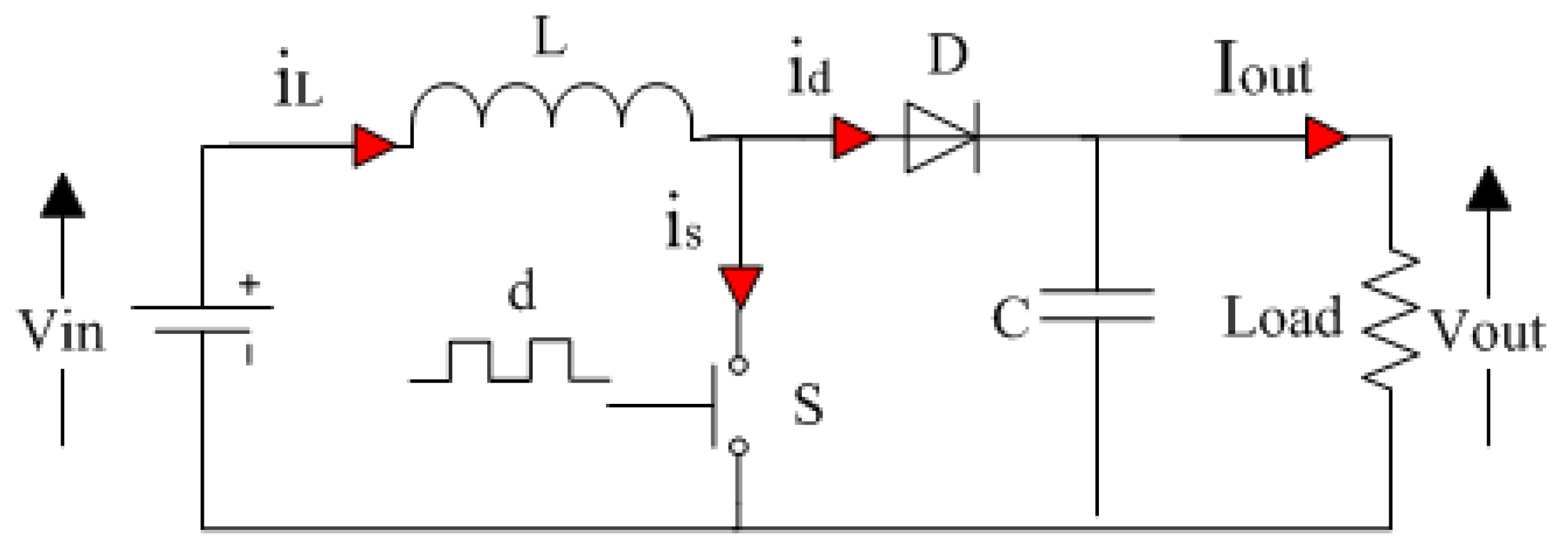
DC–DC boost converter is a high step up power converter, which is used to boost and regulate an input DC voltage. In this work, the main objective of using the boost converter is to provide an efficient power conversion from the cell stack to the load and offer a regulated output voltage. As shown in Figure 4, an ideal boost converter consists of linear (filtering capacitor C, load resistor R, and inductor L) and nonlinear (diode D, switching transistor S) elements.
According to [65,66], the relationship between input and output voltage in a boost converter is presented by Equation (15), where is the input voltage source, is the output voltage, and d is the control signal which represents the switch position:
Under continuous conduction mode (CCM), the operation of a DC–DC boost converter becomes fairly simple. Thus, using the inductor L and the two switches D and s, the circuit alternates between two states (ON and OFF) for each complete switching cycle . Each state of ON and OFF has a varying duration. The ON time can be calculated by multiplying the switching cycle with the duty cycle d. The OFF time can be found by subtracting the ON time from the complete switching cycle . The waveforms of inductor current , inductor voltage , switching current , switching voltage , and diode current are shown in Figure 5.
- The ON state: When the switch S turns ON, the inductor L connects to the DC source voltage. Therefore, the current moves across the inductor L and the transistor switch s, which results in an increase in the magnitude of and , while is approximately equal to the input voltage . On the other hand, during this state, the capacitor C discharges through the load R. The obtained differential equations of the inductor current and the output voltage are expressed as follows:
- The OFF state: When the switch S turns OFF, the inductor L connects to the capacitor C and the load R. Therefore, the current moves across the inductor L, the diode D, the capacitor C, and the load R, which results in a decrease in the magnitude of and (discharging of the inductor L into the load R and the capacitor C). During this state, is approximately equal to . The obtained differential equations of the inductor current and the output voltage are expressed as follows:
The global state-space representation of the high step-up DC–DC boost converter can be expressed in Equation (18), where , represents the inductor current, and represents the output voltage.
4. MPPT Control Design
The MPPT is an algorithm used to obtain the maximum produced power from a source of energy (PV, PEMFC). In this work, in order to keep the system running at an efficient power point, the MPPT based on the backstepping algorithm is used to drive the boost converter, which is placed between the stack cell and the load (Figure 6). The central problem addressed by the MPPT is that the PEMFC efficiency depends on the amount of supplied hydrogen, the cell temperature, and the load variations. In order to keep this efficiency at the highest value, the system must be optimized to obtain the current closest to the current at which the PEMFC characteristic gives the maximum available power. Hence, the aim of the MPPT is to find the MPP and force the PEMFC to operate at this point. Thus, it helps to overcome the difficulties of choosing the most efficient current under the influence of the inputs and the load variations. Therefore, the MPPT can be considered as the fundamental phase for obtaining good performance in a PEMFC. The MPPT control algorithm is usually based on changing the converter duty cycle d to compel the PEMFCs to function at its MPP.
In this section, the proposed MPPT method is designed based on two steps. The first is the determination of the current reference estimator (), which corresponds to the current of the MPP. For the controller, represents the reference current (), which the operating current must achieve. The second step is the development of the backstepping technique, which commands the duty cycle of the boost converter through the pulse width modulation (PDM).
4.1. Current Reference Estimator
The aim of this step is the determination of the reference current for different operating conditions. According to Figure 7, it is clearly shown that the performance of the PEMFC is largely influenced by the variation made on hydrogen, oxygen, and temperature. Thus, the hydrogen operating pressure varied from 0.01 to 0.6 bar, and oxygen operating pressure varied from 0.00022 to 0.0022 bar, while the operating temperature T varied from 25 to 50 C. When and are equal to 0.01 and 0.00022 bar, respectively, the power generated by the PEMFC is at the lowest value compared to the pressure of other gasses. On the other hand, once and increase to 0.6 and 0.0022 bar, respectively, the power produced by the PEMFC is at the highest value. Consequently, the efficiency of the PEMFC is improved by rising the partial pressures. Besides, the efficiency of the PEMFC may also be improved by raising its temperature. However, compared to the influence of the partial pressure, the PEMFC is not largely influenced by its temperature variations.
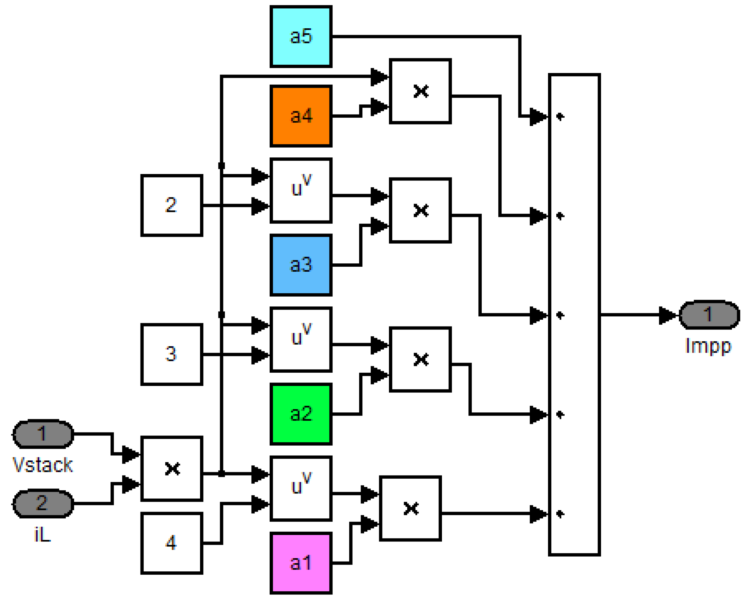
Figure 7 also shows that, for each operating temperature and pressure, the maximum power can be obtained using the MPP curve. The latter is constructed using the function given in Equation (19). The synoptic diagram of this function is shown in Figure 8. It calculates the corresponding for each MPP value. Therefore, the blue curve that has been constructed using the fitting function = is considered as the MPP reference current estimator.
where , , , and .
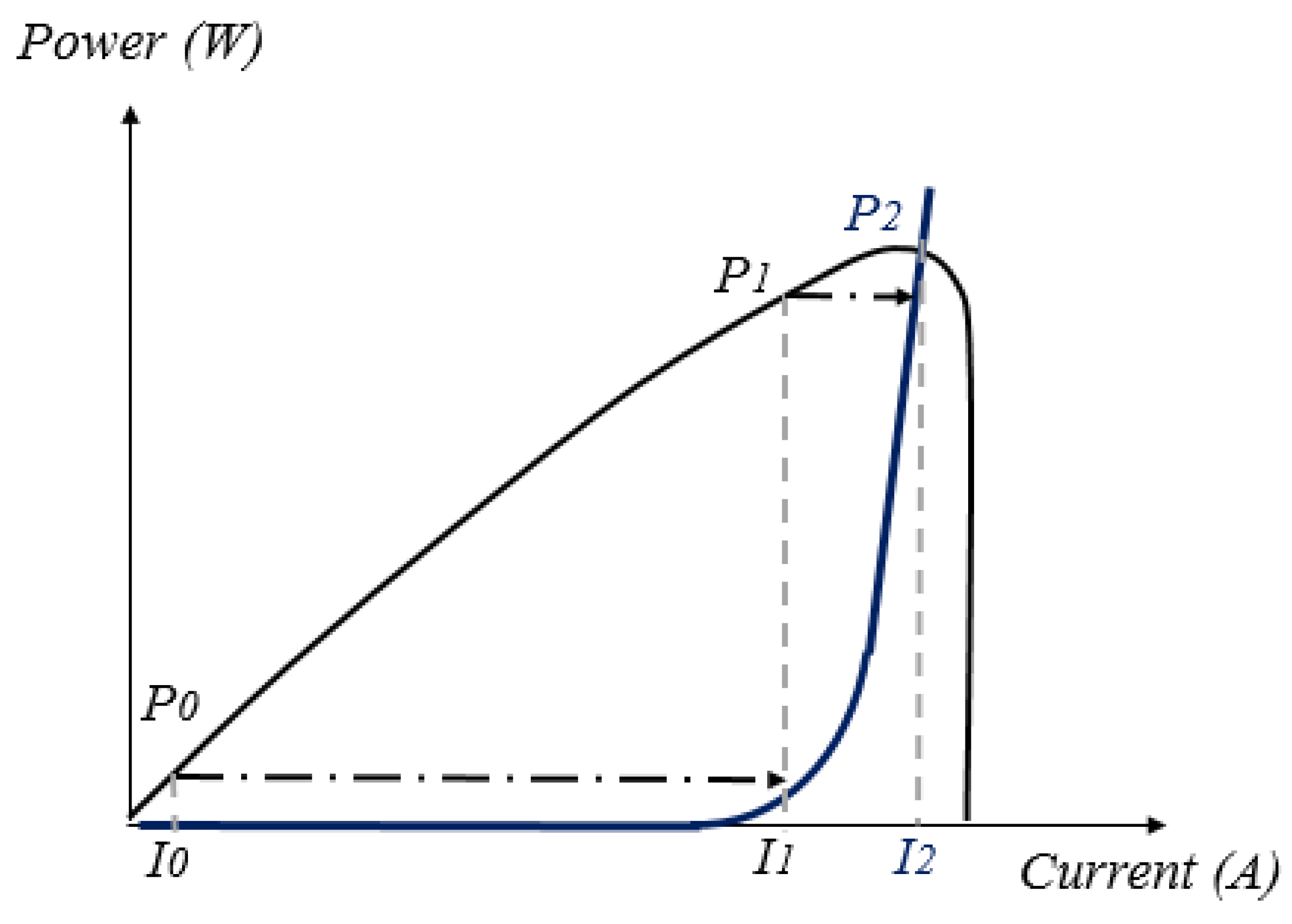
Figure 9 clarifies that, for any operating power point, after several projections, the PEMFCs will be managed to operate at the desired point and then extract the maximum power from the PEMFC. For instance, suppose that the system works at . The projection of this power point onto the blue curve will change the operating current from to . As a consequence, the system will be working at . By applying the same process on the operating power point , the system will be brought to operate at , which is closer to the MPP. After several projections, the operating power point will change repeatedly until it reaches the MPP where the reference current equals to . The main feature of this method is that we can keep the fuel cell working at its MPP with great performance.
4.2. Current Regulation
In order to track the estimated current , the PI controller and backstepping algorithm are designed to force the stack power to track the optimal point . By acting on the duty cycle of the boost converter, the operating current will be forced to track, as much as possible, the current .
4.2.1. PI Controller
The PI controller is a control loop feedback system that attempts as much as possible to continuously calculate the difference between the desired and actual (measured) outputs. The control function of the PI controller is given in Equation (20), while its synoptic diagram is shown in Figure 10, where is the error, and and are respectively the proportional and integral coefficient terms.
Although the PI controller is commonly used in a wide range of applications, several drawbacks such as the difficulties of finding out the constants and are causing a big issue [67,68,69,70]. Moreover, its sensibility dealing with the load variations has caused researchers to look for another controllers that can provide robustness against load variations. In this paper, the method used for determining the values of and is known as the “Ziegler–Nichols tuning method,” discovered and developed by J. G. Ziegler and N. B. Nichols. It is an online method that is usually used when there is a lack of knowledge of the model parameters [71]. In order to apply this method, three main steps should be accomplished.
- The first step is to switch off the integral and derivative gains ( and ).
- The second step is to increase the gain from a low/zero value until the first sustained oscillation occurs (Figure 11). The reached gain at the sustained oscillation is noted as a critical value , while the period of these oscillations is measured as .
- Finally, taking into account the type of the used controller, and can be calculated using the formula given in Table 2.
4.2.2. Backstepping Algorithm
Backstepping is a nonlinear control solution that acts in accordance with the nonlinearity of the boost converter. It is well known by its robustness against modeling inaccuracies and system parameter fluctuations. After the estimation of , the backstepping algorithm is applied to reduce as much as possible the actual current error between the desired setpoint current and the PEMFC measured current variable . Thus, the backstepping algorithm is designed to enforce to track, as accurately as possible, . The backstepping approach [52,53,54,56,57,58] is designed as follows:
- Step 1. First, we define the tracking current error asIn order to achieve the tracking objective, it is needed to enforce to vanish. Therefore, the dynamics of must be clearly defined. By placing Equation (18) into Equation (21), the time derivative of can be written aswhere the quantity is a virtual variable. In order to stabilize the virtual error , a Lyapunov function is considered:Using the equations mentioned above, the time derivative of can be represented asEquation (24) shows that can be adjusted to zero () if , where the stabilizing function is defined by Equation (25):where is a positive constant parameter. Since is a virtual variable and not the actual input of the controller, then a second tracking error variable is given by Equation (26):Using Equations (25) and (26), Equation (22) can be written asTherefore, the Lyapunov function given in Equation (24) can also be rewritten as
- Step 2. The aim of this step is to enforce the errors to vanish. For this reason, first of all, the dynamics of must be determined. Using Equations (18), (25) and (27), the time-derivative of can be obtained aswhereIn order to obtain a stabilizing control law for the whole system, the following Lyapunov function candidate is proposed:The time derivative of the above Lyapunov function is obtained by combining Equations (28) and (29):It can be easily determined that the global asymptotic stability of the equilibrium is achieved only if the time derivative of the error variable is chosen aswhere is a positive design parameter. Finally, by combining Equations (29) and (34), the following control law can be obtained:
Using the above equations, the implementation of the backstepping algorithm in the Matlab–Simulink environment is presented by Figure 12.
5. Simulation Results
In this section, the PEMFCs including the fuel cell, the boost, and the designed MPPT based on the PI and backstepping algorithm are implemented in a Matlab–Simulink environment. Comparison results between the two controllers are also analyzed and discussed in this section. The parameters values of the boost converter components and the controllers are listed in Table 3.
In order to verify the performances of the proposed MPPT method, variations in temperature, hydrogen, and load resistance are applied at different times. Thus, as shown in Figure 13, load resistance variations are performed at and s, from 20 to 100 , and from 100 to 10 , respectively, temperature variations are performed at and s, from 25 to , and from 35 to , respectively, and hydrogen variations are performed at and s, from to bar, and from to bar, respectively.
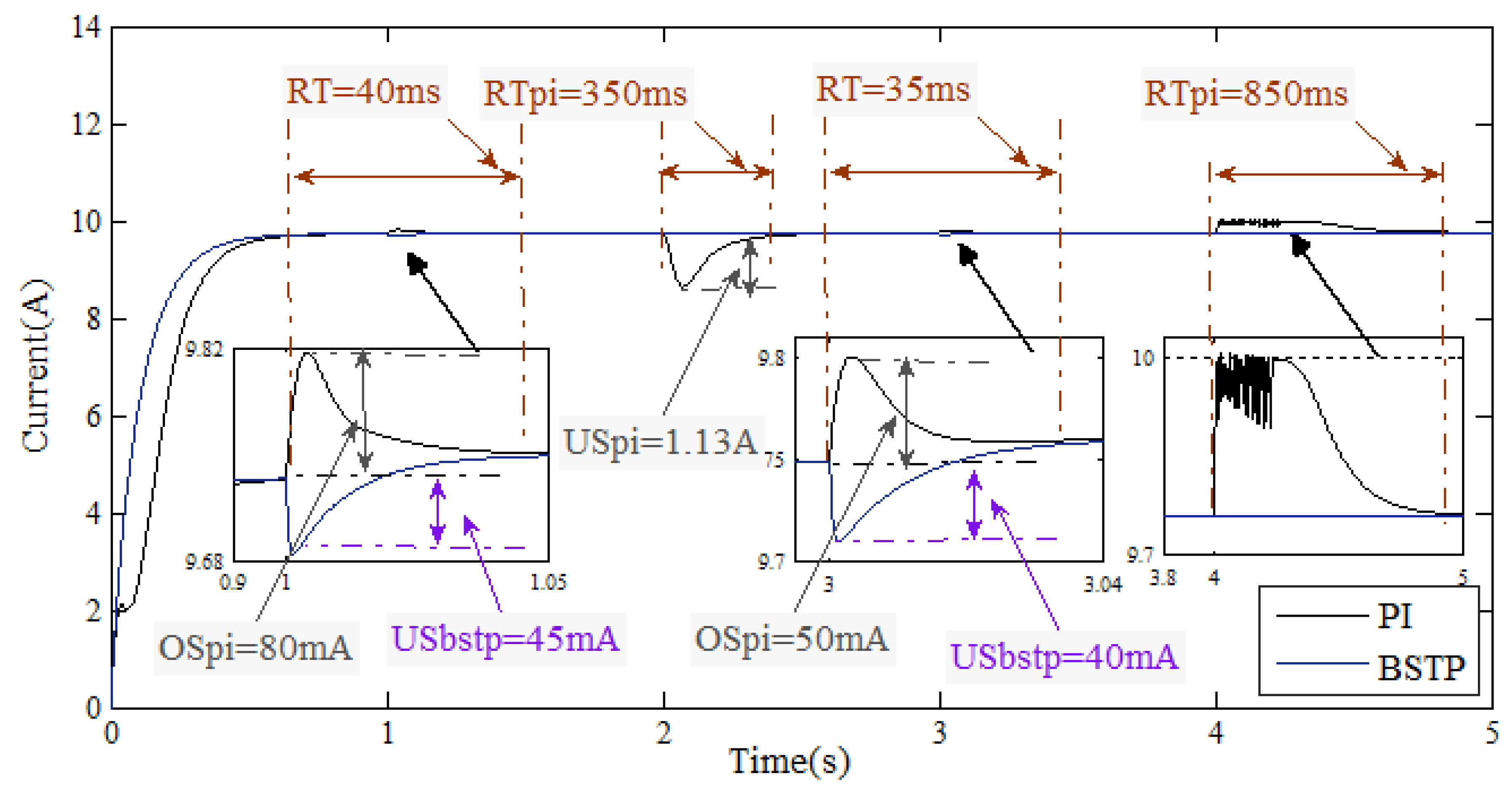
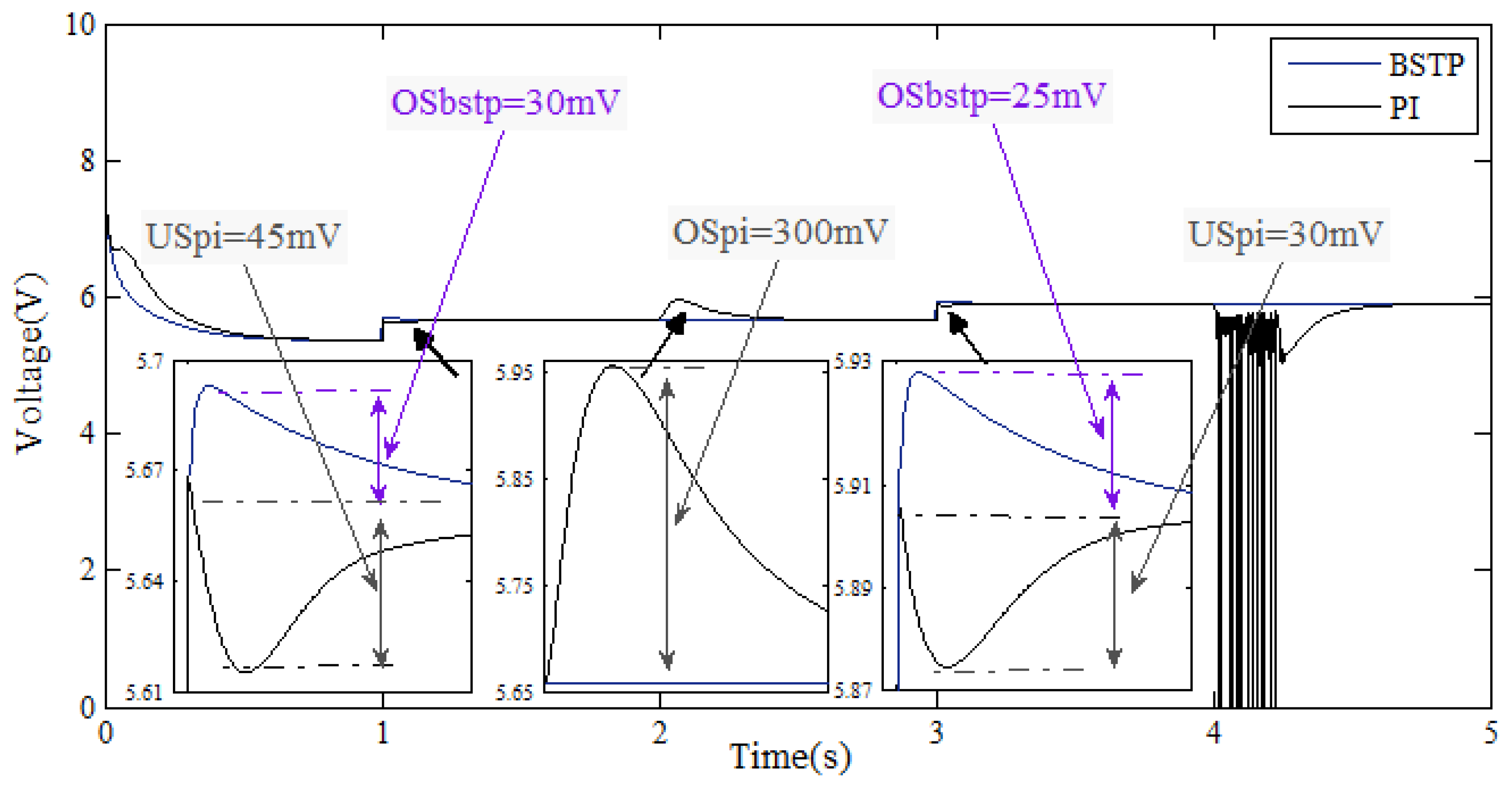
Figure 14, Figure 15 and Figure 16 show, respectively, the waveforms of the PEMFC current, voltage, and power. They illustrate the behaviour of the MPPT method based on PI and the backstepping algorithm to track the MPP under the variation of temperature, hydrogen, and load resistance. These figures confirm that the proposed MPPT shows satisfactory results for maintaining the PEMFC at high-performance operation. Hence, the proposed method manifest a gradual and smooth increase to the MPP value. It is clearly presented that, in the presence of hydrogen variations ( and s), the MPP is obtained quickly with fantastic rigor and global stability of the closed-loop system. Thus, these figures show the validity of the proposed MPPT method to keep the PEMFC generating an efficient power response. In addition, good performance such as high tracking accuracy is achieved even for large system parameter variations. On the other hand, Figure 14, Figure 15 and Figure 16 show that the proposed backstepping algorithm provides better results compared to the conventional PI controller for tracking the reference current (). Moreover, these figures show the excellent recovering features of the backstepping algorithm against load variation. The fuel cell current and voltage signals controlled by backstepping and the PI controller are respectively shown in Figure 14 and Figure 15. According to these figures, it is clearly presented that the proposed backstepping algorithm offers gradual and smooth escalations to the reference current value. It offers a fast start-up with a response time equal to 320 ms, while the PI controller takes approximately 450 ms. Furthermore, these figures illustrate the PI and backstepping behavior when facing hydrogen variations at and s, and load resistance variations at and s. It is noticeable that the backstepping technique shows better tracking performance compared to the conventional PI controller. Thus, at s, the PI shows an overshoot current of 80 mA and an undershoot voltage of 45 mV, while the backstepping shows an undershoot current of 45 mA and an overshoot voltage of 30 mV. At s, the PI shows an overshoot current of 50 mA and an undershoot voltage of 30 mV, while the backstepping shows an undershoot current of 40 mA and an overshoot voltage of 25 mV. However, these overshoots and undershoots appear only for short durations (less than 50 ms), and they quickly converge to the steady-state value. The robustness of the backstepping technique over the PI controller is clearly apparent at and s. Thus, despite the variation of the load from 20 to 100 and from 100 to 10 , the backstepping shows high robustness against these variations. On the other hand, the weakness of the conventional PI controller against load variation is clearly shown. It takes 350 ms and 850 ms response times when and s, respectively. Therefore, it should be noted that the PI controller may even cause damage to the PEMFC. Consequently, these figures demonstrate the robustness of the backstepping algorithm against load resistance variations.
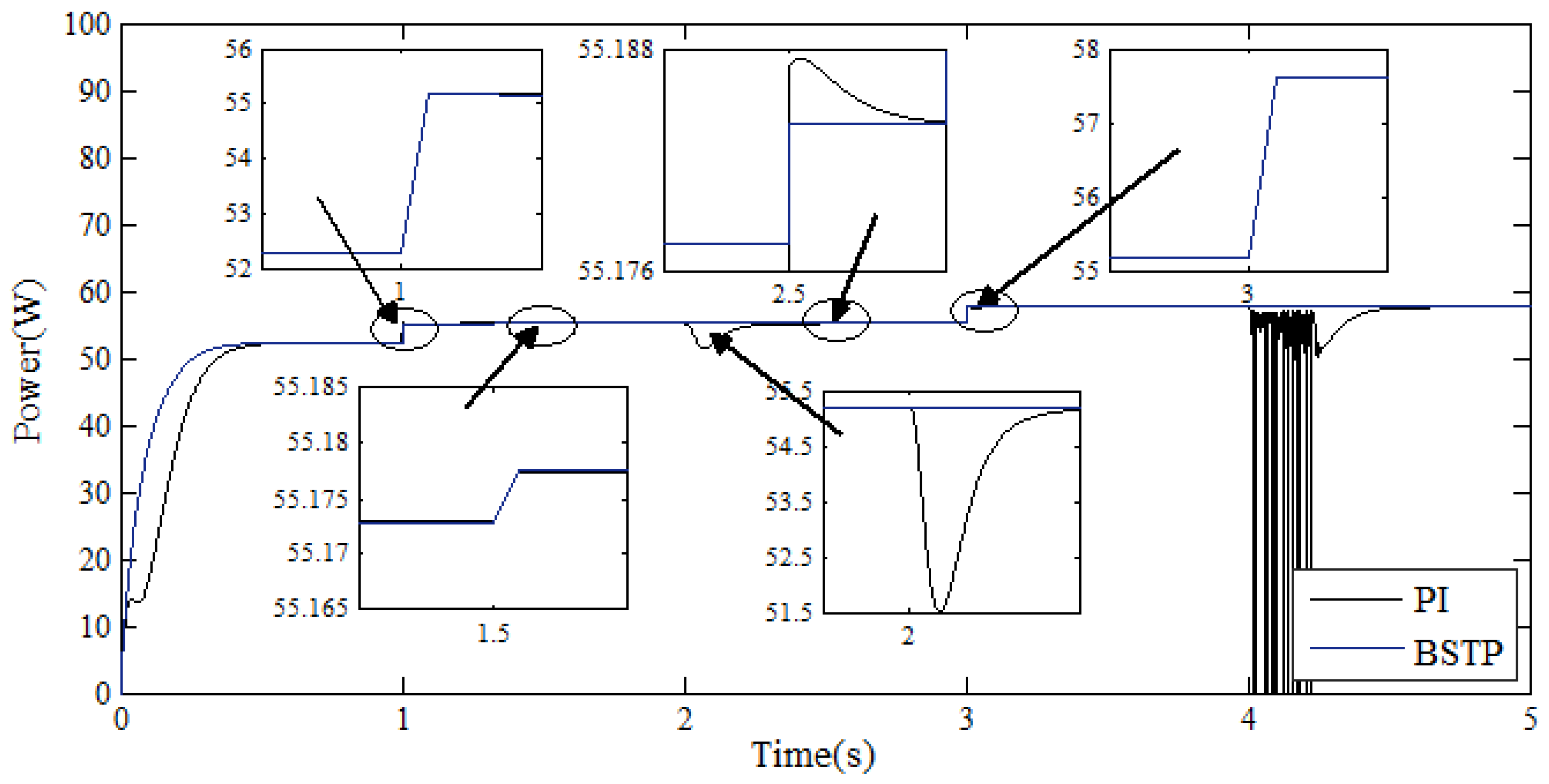
The PEMFC stack power curves are shown in Figure 16. Compared to the nominal characteristics of the PEMFC, an improvement of 12% in the fuel cell power is obtained using the proposed MPPT control scheme. In addition, although the extracted energies using the two controllers gives almost identical results (with a slight advantage for the backstepping algorithm), it is clear that, when using the backstepping technique, the MPP is obtained with high-performance motion tracking. On the other hand, in addition to its complexity, it is clear that the drawback of the PI controller is its weakness when facing load resistance variation. Consequently, the validity of the backstepping algorithm and its robustness under load resistance variations is clear. Moreover, a magnificent performance, with a quick start-up and high tracking accuracy, is obtained, even for large system parameter variations.
6. Conclusions
In this paper, a detailed mathematical model of a PEM fuel cell and a DC–DC boost converter is described, discussed, and investigated. Moreover, a detailed study of the tracking method as well as the controllers is also presented. An entire system driven by PI and the backstepping algorithm was constructed and checked using Matlab–Simulink. The performance of the fuel cell was analyzed using I-V and I-P characteristics at different hydrogen and oxygen pressures. Through an extensive simulation study, it is demonstrated that the proposed new MPPT method shows satisfactory tracking performance with respect to the maximum power point. Moreover, in comparison with PI results, it is clear that the proposed MPPT based on the backstepping technique shows superior behavior, with great robustness, a fast settling time, high control precision, and good adaptation toward external factor variations. This paper paves the way for an experimental study of the proposed feedback control scheme on a real fuel cell power system.
Author Contributions
M.D. designed the simulations, analyzed the results, and wrote the paper; O.B. and L.S. assisted in the analysis of the results and revised the manuscript for submission.
Funding
This research was funded by the UPV/EHU PPGA18/04 and by the Basque Government through the project ETORTEK KK-2017/00033.
Acknowledgments
The authors are very grateful to the UPV/EHU for its support through the projects PPGA18/04 and to the Basque Government for its support through the project ETORTEK KK-2017/00033. The authors would also like to thank the Tunisian Government for its support through the research unit UR11ES82.
Conflicts of Interest
The authors declare no conflict of interest.
Abbreviations
The following abbreviations are used in this manuscript:
| MPP | Maximum Power Point |
| MPPT | Maximum Power Point Tracker |
| PEMFCs | proton exchange membrane Fuel Cell systems |
| FSC | Fractional Short Circuit |
| P&O | Perturb and Observation |
| FOC | Fractional Open Circuit |
| Inc-Cond | Incremental Conductance |
| ESC | Extremum Seeking Control |
| SMC | Sliding Mode Control |
| CS | Current Sweep |
| FLC | Fuzzy Logic Control |
| ESC | Eagle Strategy Control |
| PSO | Particle Swarm Optimization |
| NNC | Neural Network Control |
| GA | Genetic Algorithms |
| VSIR | Variable Step-size Incremental Resistance algorithm |
| RCC | Ripple Correlation Control |
| CL | Catalyst Layer |
| GDL | Gas Diffusion Layer |
| CCM | Continuous Conduction Mode |
References
- Martin, S.S.; Chebak, A. Concept of educational renewable energy laboratory integrating wind, solar and biodiesel energies. Int. J. Hydrog. Energy 2016, 41, 21036–21046. [Google Scholar] [CrossRef]
- Roumila, Z.; Rekioua, D.; Rekioua, T. Energy management based fuzzy logic controller of hybrid system wind/photovoltaic/diesel with storage battery. Int. J. Hydrog. Energy 2017, 42, 19525–19535. [Google Scholar] [CrossRef]
- Simari, C.; Potsi, G.; Policicchio, A.; Perrotta, I.; Nicotera, I. Clay–Carbon Nanotubes Hybrid Materials for Nanocomposite Membranes: Advantages of Branched Structure for Proton Transport under Low Humidity Conditions in PEMFCs. J. Phys. Chem. C 2016, 120, 2574–2584. [Google Scholar] [CrossRef]
- Rosli, R.; Sulong, A.; Daud, W.; Zulkifley, M.; Husaini, T.; Rosli, M.; Majlan, E.; Haque, M. A review of high-temperature proton exchange membrane fuel cell (HT-PEMFC) system. Int. J. Hydrog. Energy 2017, 42, 9293–9314. [Google Scholar] [CrossRef]
- Torki, W.; Derbeli, M. Modeling and control of a stand-alone PEMFC for AC load-PMSM application. In Proceedings of the 2017 International Conference on Green Energy Conversion Systems (GECS), Hammamet, Tunisia, 23–25 March 2017; pp. 1–6. [Google Scholar] [CrossRef]
- Headley, A.; Yu, V.; Borduin, R.; Chen, D.; Li, W. Development and Experimental Validation of a Physics-Based PEM Fuel Cell Model for Cathode Humidity Control Design. IEEE/ASME Trans. Mech. 2016, 21, 1775–1782. [Google Scholar] [CrossRef]
- Sher, H.A.; Murtaza, A.F.; Noman, A.; Addoweesh, K.E.; Al-Haddad, K.; Chiaberge, M. A new sensorless hybrid MPPT algorithm based on fractional short-circuit current measurement and P&O MPPT. IEEE Trans. Sustain. Energy 2015, 6, 1426–1434. [Google Scholar] [CrossRef]
- Bharath, K.; Suresh, E. Design and Implementation of Improved Fractional Open Circuit Voltage Based Maximum Power Point Tracking Algorithm for Photovoltaic Applications. Int. J. Renew. Energy Res. (IJRER) 2017, 7, 1108–1113. [Google Scholar]
- Gosumbonggot, J. Maximum power point tracking method using perturb and observe algorithm for small scale DC voltage converter. Proc. Comput. Sci. 2016, 86, 421–424. [Google Scholar] [CrossRef]
- Derbeli, M.; Sbita, L.; Farhat, M.; Barambones, O. Proton exchange membrane fuel cell—A smart drive algorithm. In Proceedings of the 2017 International Conference on Green Energy Conversion Systems (GECS), Hammamet, Tunisia, 23–25 March 2017; pp. 1–5. [Google Scholar] [CrossRef]
- Serrano-Guerrero, X.; González-Romero, J.; Cárdenas-Carangui, X.; Escrivá-Escrivá, G. Improved variable step size P&O MPPT algorithm for PV systems. In Proceedings of the 2016 51st International Universities Power Engineering Conference (UPEC), Coimbra, Portugal, 6–9 September 2016; pp. 1–6. [Google Scholar] [CrossRef]
- Sarvi, M.; Barati, M. Voltage and current based MPPT of fuel cells under variable temperature conditions. In Proceedings of the 2010 45th International Universities Power Engineering Conference (UPEC), Cardiff, UK, 31 August–3 September 2010; pp. 1–4. [Google Scholar]
- Chen, P.Y.; Yu, K.N.; Yau, H.T.; Li, J.T.; Liao, C.K. A novel variable step size fractional order incremental conductance algorithm to maximize power tracking of fuel cells. Appl. Math. Model. 2017, 45, 1067–1075. [Google Scholar] [CrossRef]
- Harrag, A.; Messalti, S. Variable Step Size IC MPPT Controller for PEMFC Power System Improving Static and Dynamic Performances. Fuel Cells 2017, 17, 816–824. [Google Scholar] [CrossRef]
- Cecati, C.; Khalid, H.A.; Tinari, M.; Adinolfi, G.; Graditi, G. DC nanogrid for renewable sources with modular DC/DC LLC converter building block. IET Power Electron. 2016, 10, 536–544. [Google Scholar] [CrossRef]
- Bizon, N.; Thounthong, P.; Raducu, M.; Constantinescu, L.M. Designing and modelling of the asymptotic perturbed extremum seeking control scheme for tracking the global extreme. Int. J. Hydrog. Energy 2017, 42, 17632–17644. [Google Scholar] [CrossRef]
- Bizon, N. Energy optimization of fuel cell system by using global extremum seeking algorithm. Appl. Energy 2017, 206, 458–474. [Google Scholar] [CrossRef]
- Jiao, J.; Cui, X. A real-time tracking control of fuel cell power systems for maximum power point. J. Comput. Inf. Syst. 2013, 9, 1933–1941. [Google Scholar]
- Liu, J.; Zhao, T.; Chen, Y. Maximum power point tracking of proton exchange membrane fuel cell with fractional order filter and extremum seeking control. In Proceedings of the ASME 2015 International Design Engineering Technical Conferences and Computers and Information in Engineering Conference, Houston, TX, USA, 13–19 November 2015. [Google Scholar] [CrossRef]
- Derbeli, M.; Sbita, L.; Farhat, M.; Barambones, O. PEM fuel cell green energy generation—SMC efficiency optimization. In Proceedings of the 2017 International Conference on Green Energy Conversion Systems (GECS), Hammamet, Tunisia, 23–25 March 2017; pp. 1–5. [Google Scholar] [CrossRef]
- Mrad, I.; Derheli, M.; Shita, L.; Barhot, J.P.; Farhat, M.; Baramhones, O. Sensorless and robust PEMFEC power system drive based on Z (Tn) observability. In Proceedings of the 2017 International Conference on Green Energy Conversion Systems (GECS), Hammamet, Tunisia, 23–25 March 2017; pp. 1–6. [Google Scholar] [CrossRef]
- Hahm, J.; Kang, H.; Baek, J.; Lee, H.; Park, M. Design of incremental conductance sliding mode MPPT control applied by integrated photovoltaic and proton exchange membrane fuel cell system under various operating conditions for BLDC motor. Int. J. Photoenergy 2015, 2015. [Google Scholar] [CrossRef]
- Fang, Y.; Zhu, Y.; Fei, J. Adaptive Intelligent Sliding Mode Control of a Photovoltaic Grid-Connected Inverter. Appl. Sci. 2018, 8, 1756. [Google Scholar] [CrossRef]
- Tsang, K.; Chan, W. Maximum power point tracking for PV systems under partial shading conditions using current sweeping. Energy Convers. Manag. 2015, 93, 249–258. [Google Scholar] [CrossRef]
- Derbeli, M.; Mrad, I.; Sbita, L.; Barambones, O. PEM fuel cell efficiency boosting—Robust MPP tracking. In Proceedings of the 2018 9th International Renewable Energy Congress (IREC), Hammamet, Tunisia, 20–22 March 2018; pp. 1–5. [Google Scholar] [CrossRef]
- Benchouia, N.E.; Derghal, A.; Mahmah, B.; Madi, B.; Khochemane, L.; Aoul, E.H. An adaptive fuzzy logic controller (AFLC) for PEMFC fuel cell. Int. J. Hydrog. Energy 2015, 40, 13806–13819. [Google Scholar] [CrossRef]
- Robles Algarín, C.; Taborda Giraldo, J.; Rodríguez Álvarez, O. Fuzzy logic based MPPT controller for a PV system. Energies 2017, 10, 2036. [Google Scholar] [CrossRef]
- Na, W.; Chen, P.; Kim, J. An improvement of a Fuzzy Logic-Controlled maximum power point tracking algorithm for photovoltic applications. Appl. Sci. 2017, 7, 326. [Google Scholar] [CrossRef]
- Macaulay, J.; Zhou, Z. A Fuzzy Logical-Based Variable Step Size P&O MPPT Algorithm for Photovoltaic System. Energies 2018, 11, 1340. [Google Scholar] [CrossRef]
- Rezoug, M.R.; Chenni, R.; Taibi, D. Fuzzy Logic-Based Perturb and Observe Algorithm with Variable Step of a Reference Voltage for Solar Permanent Magnet Synchronous Motor Drive System Fed by Direct-Connected Photovoltaic Array. Energies 2018, 11, 462. [Google Scholar] [CrossRef]
- Avanaki, I.N.; Sarvi, M. A new maximum power point tracking method for PEM fuel cells based on water cycle algorithm. J. Renew. Energy Environ. 2016, 3, 35. [Google Scholar]
- Fathabadi, H. Novel highly accurate universal maximum power point tracker for maximum power extraction from hybrid fuel cell/photovoltaic/wind power generation systems. Energy 2016, 116, 402–416. [Google Scholar] [CrossRef]
- Mohapatra, A.; Nayak, B.; Das, P.; Mohanty, K.B. A review on MPPT techniques of PV system under partial shading condition. Renew. Sustain. Energy Rev. 2017, 80, 854–867. [Google Scholar] [CrossRef]
- Karami, N.; Moubayed, N.; Outbib, R. General review and classification of different MPPT Techniques. Renew. Sustain. Energy Rev. 2017, 68, 1–18. [Google Scholar] [CrossRef]
- Sarvi, M.; Parpaei, M.; Soltani, I.; Taghikhani, M. Eagle strategy based maximum power point tracker for fuel cell system. Int. J. Eng.-Trans. A Basics 2015, 28, 529–536. [Google Scholar]
- Kim, M.K. Optimal control and operation strategy for wind turbines contributing to grid primary frequency regulation. Appl. Sci. 2017, 7, 927. [Google Scholar] [CrossRef]
- Kalaiarasi, N.; Dash, S.S.; Padmanaban, S.; Paramasivam, S.; Morati, P.K. Maximum Power Point Tracking Implementation by Dspace Controller Integrated Through Z-Source Inverter Using Particle Swarm Optimization Technique for Photovoltaic Applications. Appl. Sci. 2018, 8, 145. [Google Scholar] [CrossRef]
- Pohjoranta, A.; Sorrentino, M.; Pianese, C.; Amatruda, F.; Hottinen, T. Validation of neural network-based fault diagnosis for multi-stack fuel cell systems: Stack voltage deviation detection. Energy Procedia 2015, 81, 173–181. [Google Scholar] [CrossRef]
- Bicer, Y.; Dincer, I.; Aydin, M. Maximizing performance of fuel cell using artificial neural network approach for smart grid applications. Energy 2016, 116, 1205–1217. [Google Scholar] [CrossRef]
- Chen, M.; Ma, S.; Wu, J.; Huang, L. Analysis of MPPT failure and development of an augmented nonlinear controller for MPPT of photovoltaic systems under partial shading conditions. Appl. Sci. 2017, 7, 95. [Google Scholar] [CrossRef]
- Hadji, S.; Gaubert, J.P.; Krim, F. Real-Time Genetic Algorithms-Based MPPT: Study and Comparison (Theoretical an Experimental) with Conventional Methods. Energies 2018, 11, 459. [Google Scholar] [CrossRef]
- Adinolfi, G.; Graditi, G.; Siano, P.; Piccolo, A. Multiobjective optimal design of photovoltaic synchronous boost converters assessing efficiency, reliability, and cost savings. IEEE Trans. Ind. Inform. 2015, 11, 1038–1048. [Google Scholar] [CrossRef]
- Xiao, W.; Dunford, W.G.; Palmer, P.R.; Capel, A. Application of centered differentiation and steepest descent to maximum power point tracking. IEEE Trans. Ind. Electron. 2007, 54, 2539–2549. [Google Scholar] [CrossRef]
- Tolentino, L.K.S.; Cruz, F.R.G.; Garcia, R.G.; Chung, W.Y. Maximum power point tracking controller IC based on ripple correlation control algorithm. In Proceedings of the 2015 International Conference on Humanoid, Nanotechnology, Information Technology, Communication and Control, Environment and Management (HNICEM), Cebu City, Philippines, 9–12 December 2015; pp. 1–6. [Google Scholar] [CrossRef]
- Ferdous, S.; Shafiullah, G.; Oninda, M.A.M.; Shoeb, M.A.; Jamal, T. Close loop compensation technique for high performance MPPT using ripple correlation control. In Proceedings of the 2017 Australasian Universities Power Engineering Conference (AUPEC), Melbourne, Australia, 19–22 November 2017; pp. 1–6. [Google Scholar] [CrossRef]
- Hammami, M.; Grandi, G. A Single-Phase Multilevel PV Generation System with an Improved Ripple Correlation Control MPPT Algorithm. Energies 2017, 10, 2037. [Google Scholar] [CrossRef]
- Benhalima, S.; Miloud, R.; Chandra, A. Real-Time Implementation of Robust Control Strategies Based on Sliding Mode Control for Standalone Microgrids Supplying Non-Linear Loads. Energies 2018, 11, 2590. [Google Scholar] [CrossRef]
- Martin, A.D.; Cano, J.; Silva, J.F.A.; Vázquez, J.R. Backstepping control of smart grid-connected distributed photovoltaic power supplies for telecom equipment. IEEE Trans. Energy Convers. 2015, 30, 1496–1504. [Google Scholar] [CrossRef]
- Patra, S.; Ankur Narayana, M.; Mohanty, S.R.; Kishor, N. Power quality improvement in grid-connected photovoltaic—Fuel cell based hybrid system using robust maximum power point tracking controller. Electr. Power Compon. Syst. 2015, 43, 2235–2250. [Google Scholar] [CrossRef]
- Taouni, A.; Abbou, A.; Akherraz, M.; Ouchatti, A.; Majdoul, R. MPPT design for photovoltaic system using backstepping control with boost converter. In Proceedings of the 2016 International Renewable and Sustainable Energy Conference (IRSEC), Marrakech, Morocco, 14–17 November 2016; pp. 469–475. [Google Scholar] [CrossRef]
- Reddak, M.; Berdai, A.; Gourma, A.; Belfqih, A. Integral backstepping control based maximum power point tracking strategy for wind turbine systems driven DFIG. In Proceedings of the 2016 International Conference on Electrical and Information Technologies (ICEIT), Paris, France, 17–18 March 2016; pp. 84–88. [Google Scholar] [CrossRef]
- Wu, D.; Chen, M.; Gong, H.; Wu, Q. Robust Backstepping Control of Wing Rock Using Disturbance Observer. Appl. Sci. 2017, 7, 219. [Google Scholar] [CrossRef]
- Chen, L.H.; Peng, C.C. Extended backstepping sliding controller design for chattering attenuation and its application for servo motor control. Appl. Sci. 2017, 7, 220. [Google Scholar] [CrossRef]
- Lee, K.U.; Choi, Y.H.; Park, J.B. Backstepping Based Formation Control of Quadrotors with the State Transformation Technique. Appl. Sci. 2017, 7, 1170. [Google Scholar] [CrossRef]
- Nafaa, H.; Farhat, M.; Lassaad, S. A PV water desalination system using backstepping approach. In Proceedings of the 2017 International Conference on Green Energy Conversion Systems (GECS), Hammamet, Tunisia, 23–25 March 2017; pp. 1–5. [Google Scholar] [CrossRef]
- Guo, Q.; Liu, Y.; Jiang, D.; Wang, Q.; Xiong, W.; Liu, J.; Li, X. Prescribed Performance Constraint Regulation of Electrohydraulic Control Based on Backstepping with Dynamic Surface. Appl. Sci. 2018, 8, 76. [Google Scholar] [CrossRef]
- Duan, K.; Fong, S.; Zhuang, Y.; Song, W. Artificial Neural Networks in Coordinated Control of Multiple Hovercrafts with Unmodeled Terms. Appl. Sci. 2018, 8, 862. [Google Scholar] [CrossRef]
- Wang, S.; Wang, L.; Qiao, Z.; Li, F. Optimal Robust Control of Path Following and Rudder Roll Reduction for a Container Ship in Heavy Waves. Appl. Sci. 2018, 8, 1631. [Google Scholar] [CrossRef]
- Arsalan, M.; Iftikhar, R.; Ahmad, I.; Hasan, A.; Sabahat, K.; Javeria, A. MPPT for photovoltaic system using nonlinear backstepping controller with integral action. Sol. Energy 2018, 170, 192–200. [Google Scholar] [CrossRef]
- Wilberforce, T.; El-Hassan, Z.; Khatib, F.; Al Makky, A.; Baroutaji, A.; Carton, J.G.; Thompson, J.; Olabi, A.G. Modelling and simulation of Proton Exchange Membrane fuel cell with serpentine bipolar plate using MATLAB. Int. J. Hydrog. Energy 2017, 42, 25639–25662. [Google Scholar] [CrossRef]
- Rismanchi, B.; Akbari, M. Performance prediction of proton exchange membrane fuel cells using a three-dimensional model. Int. J. Hydrog. Energy 2008, 33, 439–448. [Google Scholar] [CrossRef]
- Handbook, F.C. US Department of Energy, Office of Fossil Energy, and National Energy Technology Laboratory, EG&G Technical Services; Science Application International Corporation: Reston, VA, USA, 2002. [Google Scholar]
- Larminie, J.; Dicks, A. Fuel Cell Systems Explained; John willey & Sons, Ltd.: West Sussex, UK, 2000. [Google Scholar]
- Derbeli, M.; Farhat, M.; Barambones, O.; Sbita, L. Control of PEM fuel cell power system using sliding mode and super-twisting algorithms. Int. J. Hydrog. Energy 2017, 42, 8833–8844. [Google Scholar] [CrossRef]
- Kolli, A.; Gaillard, A.; De Bernardinis, A.; Bethoux, O.; Hissel, D.; Khatir, Z. A review on DC/DC converter architectures for power fuel cell applications. Energy Convers. Manag. 2015, 105, 716–730. [Google Scholar] [CrossRef]
- Boukrich, N.; Derbeli, M.; Farhat, M.; Sbita, L. Smart auto-tuned regulators in electric vehicule PMSM drives. In Proceedings of the 2017 International Conference on Green Energy Conversion Systems (GECS), Hammamet, Tunisia, 23–25 March 2017; pp. 1–5. [Google Scholar] [CrossRef]
- Harahap, C.R.; Hanamoto, T. Fictitious Reference Iterative Tuning-Based Two-Degrees-of-Freedom Method for Permanent Magnet Synchronous Motor Speed Control Using FPGA for a High-Frequency SiC MOSFET InverterMOSFET Inverter. Appl. Sci. 2016, 6, 387. [Google Scholar] [CrossRef]
- Espíndola-López, E.; Gómez-Espinosa, A.; Carrillo-Serrano, R.V.; Jáuregui-Correa, J.C. Fourier series learning control for torque ripple minimization in permanent magnet synchronous motors. Appl. Sci. 2016, 6, 254. [Google Scholar] [CrossRef]
- Chen, J.H.; Yau, H.T.; Lu, J.H. Implementation of FPGA-based charge control for a self-sufficient solar tracking power supply system. Appl. Sci. 2016, 6, 41. [Google Scholar] [CrossRef]
- Rosyadi, M.; Muyeen, S.; Takahashi, R.; Tamura, J. A design fuzzy logic controller for a permanent magnet wind generator to enhance the dynamic stability of wind farms. Appl. Sci. 2012, 2, 780–800. [Google Scholar] [CrossRef]
- Ho, T.J.; Chang, C.H. Robust Speed Tracking of Induction Motors: An Arduino-Implemented Intelligent Control Approach. Appl. Sci. 2018, 8, 159. [Google Scholar] [CrossRef]
Figure 1.
Fuel cell operation diagram.
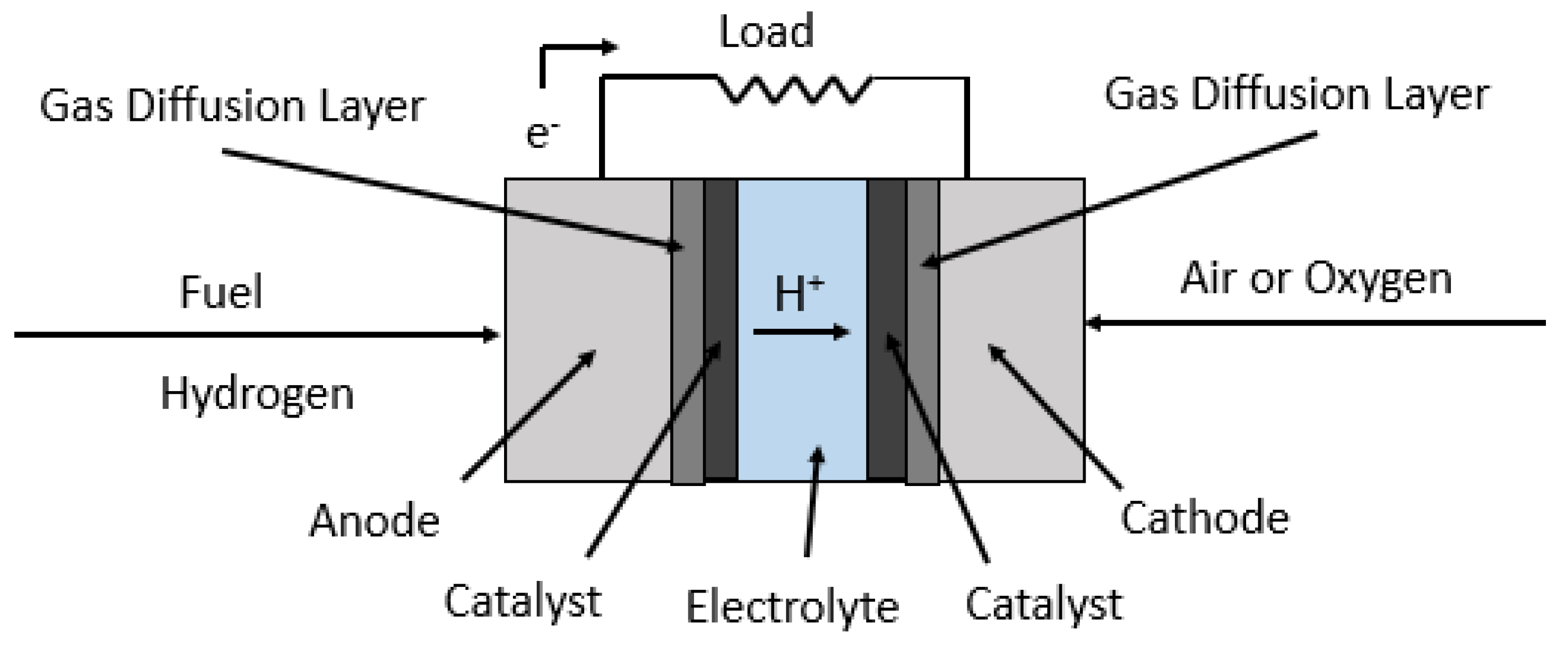
Figure 2.
Ideal and actual V-I characteristics of the PEM fuel cell (PEMFC).

Figure 3.
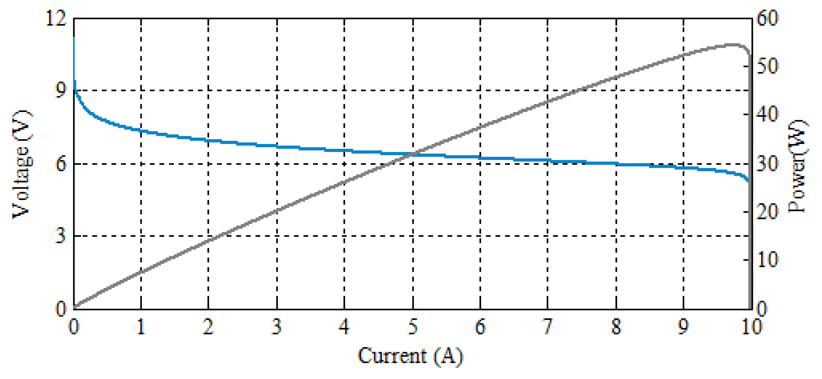
PEMFC 10 stack V-I and proportional–integral (PI) characteristics.

Figure 4.
Ideal boost converter circuit.

Figure 5.
Waveforms of different currents and voltages under continuous conduction mode (CCM) operation.
Figure 5.
Waveforms of different currents and voltages under continuous conduction mode (CCM) operation.
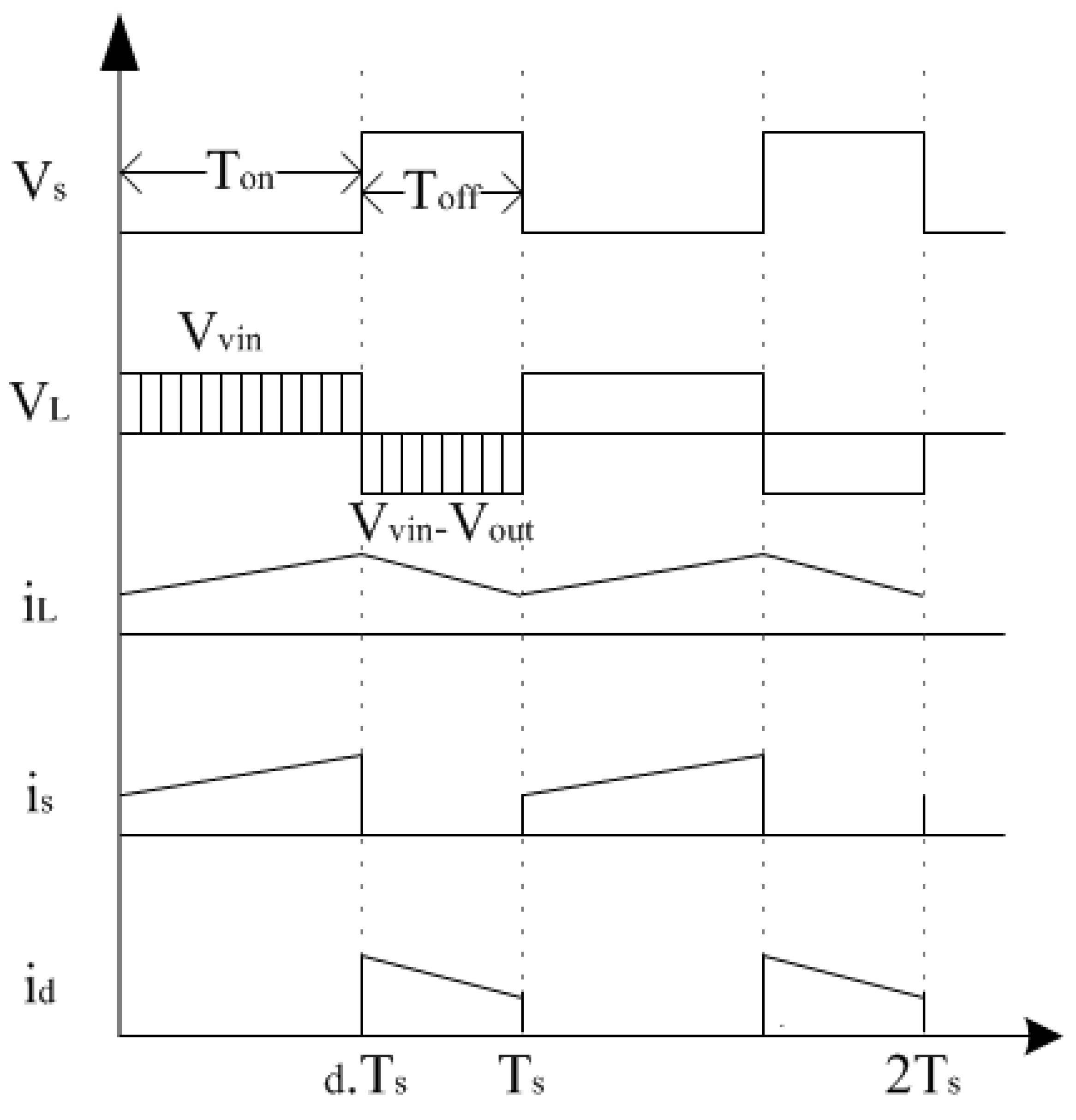
Figure 6.
Overview of the designed maximum power point tracking control.
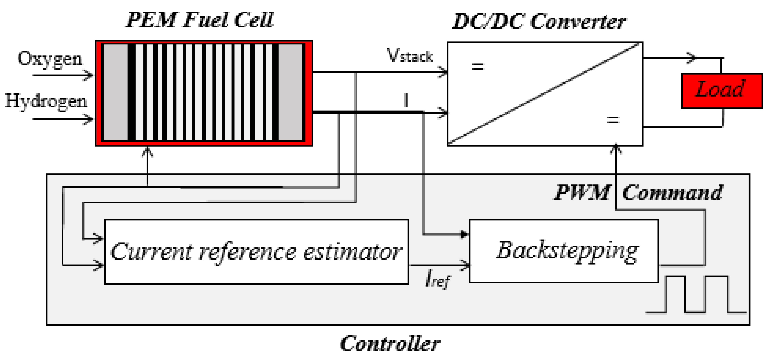
Figure 7.
The effect of the operation pressure and temperature on the PI polarization curves.
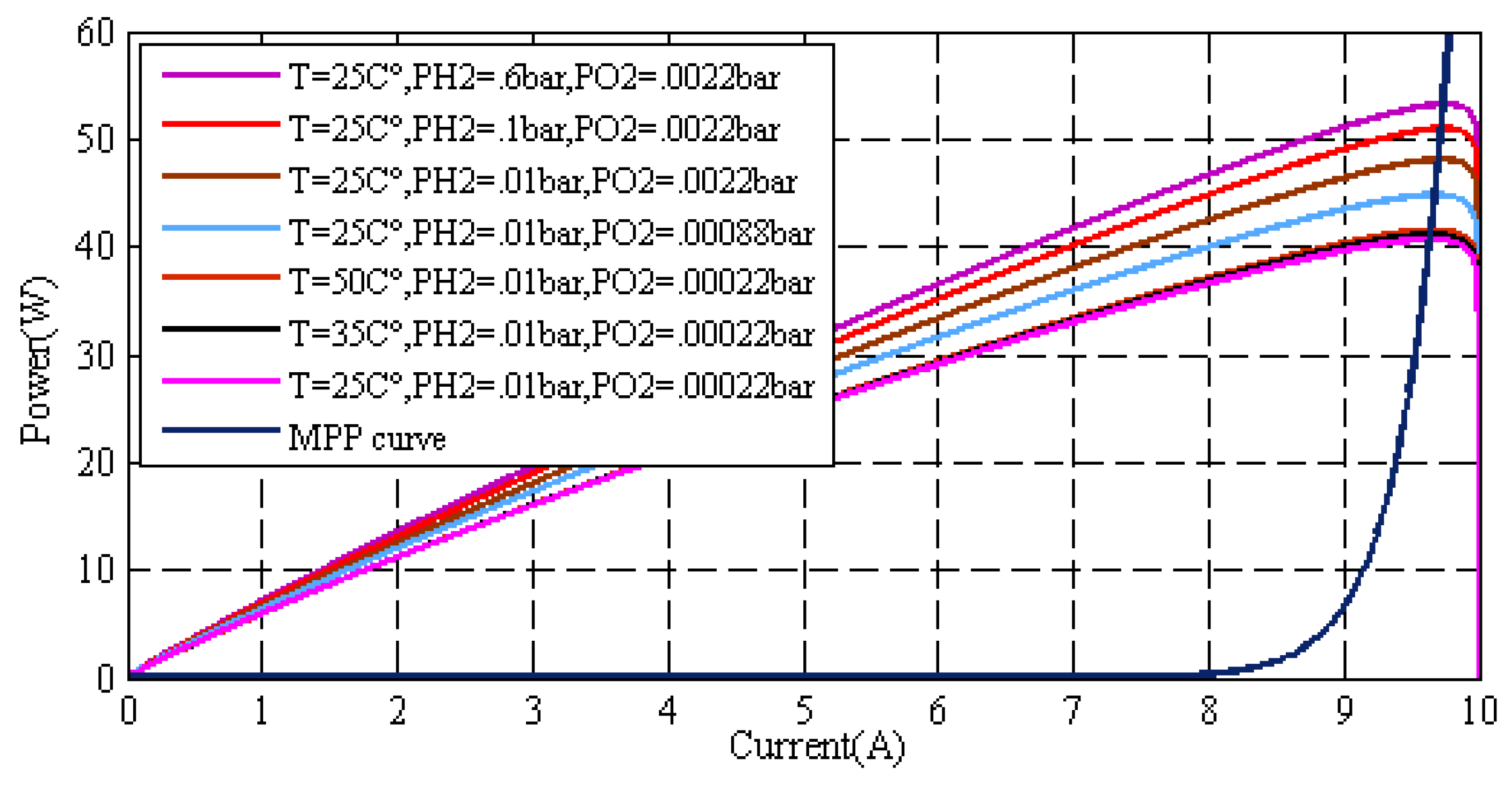
Figure 8.
Synoptic diagram of the maximum power point tracking function.

Figure 9.
PEMFC PI characteristics and tracking trajectory.

Figure 10.
Synoptic diagram of the PI controlller.
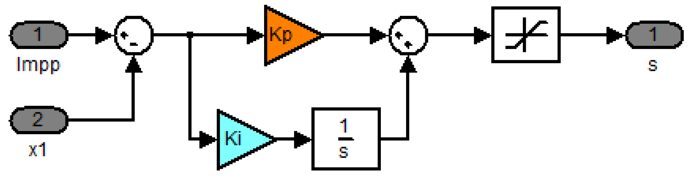
Figure 11.
Sustained oscillation with a period .
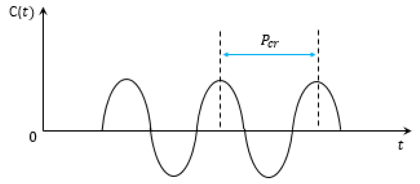
Figure 12.
Synoptic diagram of the backstepping algorithm.
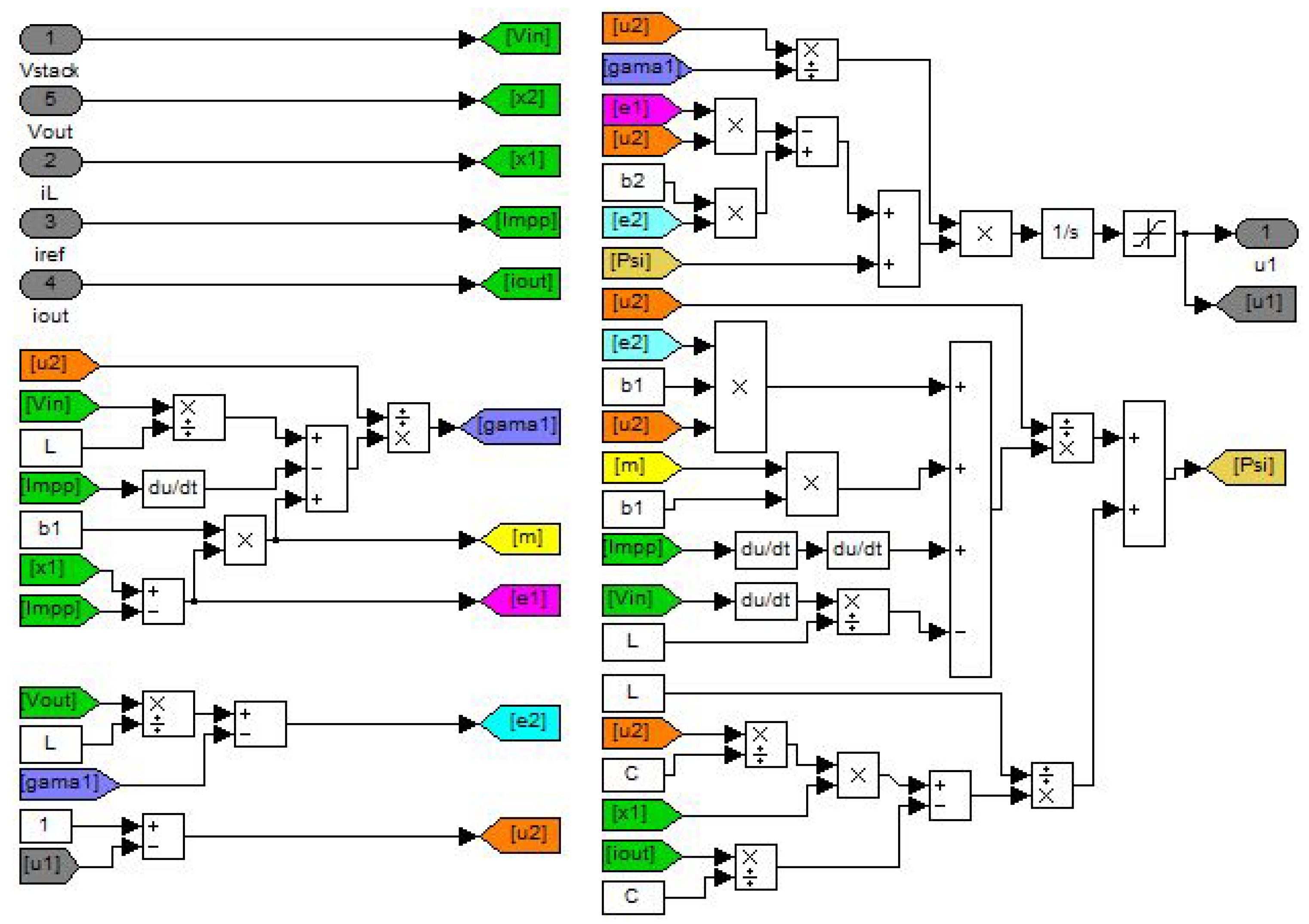
Figure 13.
Load, temperature, and hydrogen variations.
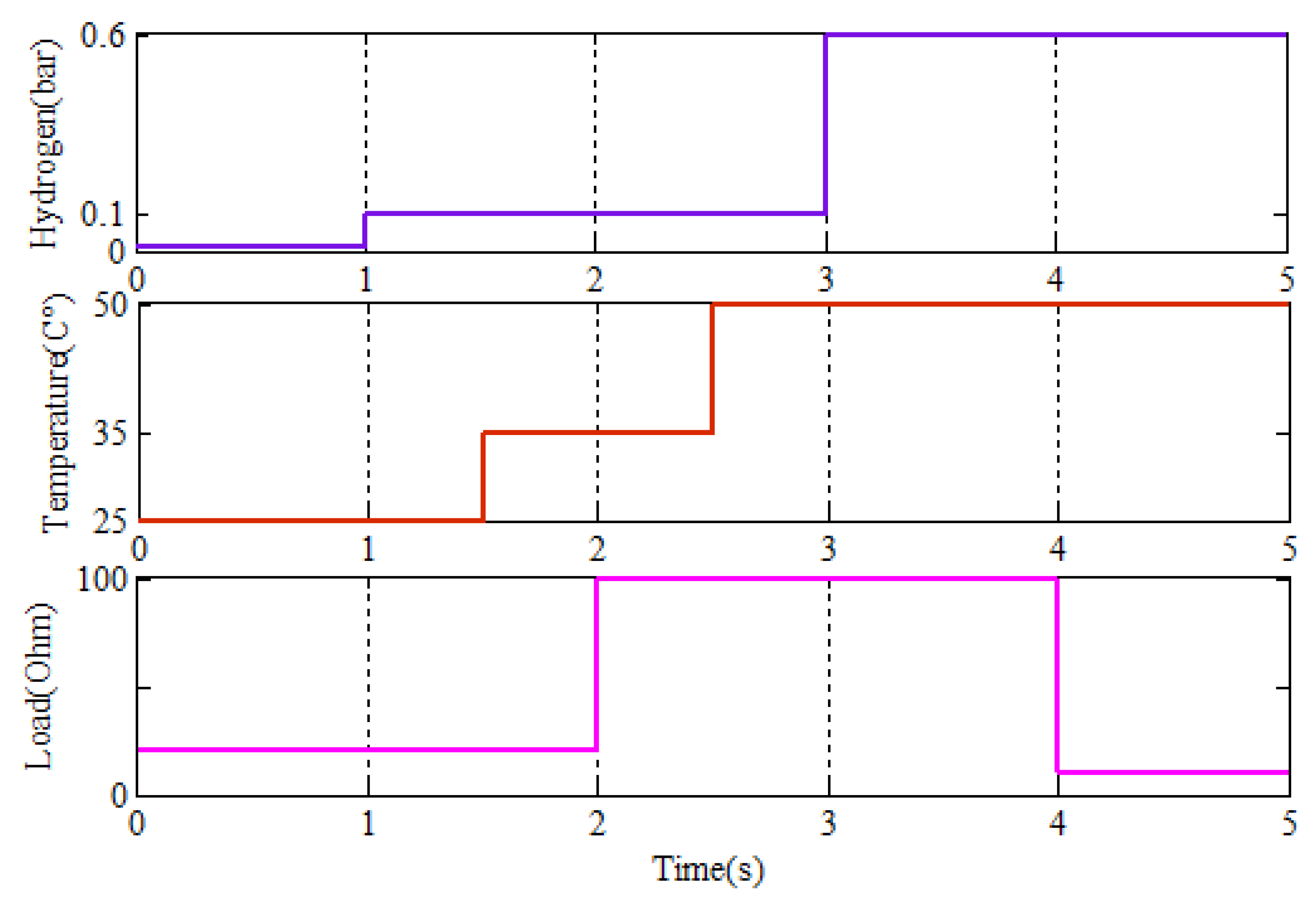
Figure 14.
PEM fuel cell stack current.

Figure 15.
PEM fuel cell stack voltage.

Figure 16.
PEM fuel cell stack power.


Table 1.
Parameter explanations of the PEMFC model.
| Parameter | Symbole | Value |
|---|---|---|
| Cell operating temperature | T | [K] |
| Cell standard temperature | 298.15 [K] | |
| Cell operating current | I | [A] |
| Universal constant of the gases | R | 83.143 [JmolK] |
| Constant of Faraday | F | 96,485.309 [Cmol] |
| Maximum current density | 0.062 A cm | |
| Current density | J | [Acm] |
| Change in the free Gibbs energy | [Jmol] | |
| Change of entropy | [Jmol] | |
| Enthalpy of formation | −285.84 kJmol | |
| Change in the Gibbs free energy at standard condition | [Jmol] | |
| Change of entropy at standard condition | [Jmol] | |
| Electrochemical thermodynamics potential | E | [V] |
| Standard potential of the fuel cell | 1.229 [V] | |
| Membrane active area | A | [162 cm] |
| Hydrogen and oxygen partial pressures | , | [atm] |
| Oxygen concentration | [molcm] | |
| Fuel cell voltage | [V] | |
| Activation losses | [V] | |
| Ohmic losses | [V] | |
| Concentration losses | [V] | |
| Constant parameters | 0.1 [V] | |
| Electric charge | Q | [coulombs] |
| Equivalent resistance of the electron flow | ||
| Proton resistance | ||
| Parametric coefficients | , , , |
Table 2.
Ziegler–Nichols tuning rules.
| Type of Controller | |||
|---|---|---|---|
| P | /2 | ∞ | 0 |
| PI | /2.2 | /1.2 | 0 |
| PID | /1.7 | /2 | /8 |
Table 3.
Boost converter components and controller parameters.
| Ideal DC–DC Boost Converter | PI Controller | Backstepping | |||||
|---|---|---|---|---|---|---|---|
| Parameter | R | L | C | ||||
| Value | 20 | H | F | 9 | 220 | ||
© 2018 by the authors. Licensee MDPI, Basel, Switzerland. This article is an open access article distributed under the terms and conditions of the Creative Commons Attribution (CC BY) license (http://creativecommons.org/licenses/by/4.0/).
Share and Cite
MDPI and ACS Style
Derbeli, M.; Barambones, O.; Sbita, L. A Robust Maximum Power Point Tracking Control Method for a PEM Fuel Cell Power System. Appl. Sci. 2018, 8, 2449. https://doi.org/10.3390/app8122449
AMA Style
Derbeli M, Barambones O, Sbita L. A Robust Maximum Power Point Tracking Control Method for a PEM Fuel Cell Power System. Applied Sciences. 2018; 8(12):2449. https://doi.org/10.3390/app8122449
Chicago/Turabian StyleDerbeli, Mohamed, Oscar Barambones, and Lassaad Sbita. 2018. "A Robust Maximum Power Point Tracking Control Method for a PEM Fuel Cell Power System" Applied Sciences 8, no. 12: 2449. https://doi.org/10.3390/app8122449
Note that from the first issue of 2016, this journal uses article numbers instead of page numbers. See further details here.