Tongue–Computer Interface Prototype Design Based on T-Type Magnet Localization for Smart Environment Control


1
School of Mechanical Engineering, University of Shanghai for Science and Technology, Shanghai 200093, China
2
State Key Laboratory of Fluid Power and Mechatronic Systems, School of Mechanical Engineering, Zhejiang University, Hangzhou 310027, China
*
Author to whom correspondence should be addressed.
Appl. Sci. 2018, 8(12), 2498; https://doi.org/10.3390/app8122498
Submission received: 8 November 2018
/
Revised: 26 November 2018
/
Accepted: 29 November 2018
/
Published: 5 December 2018
(This article belongs to the Special Issue Advanced Internet of Things for Smart Infrastructure System)
Abstract
:The interactions between paralyzed individuals with severe physical disabilities and smart infrastructure need to be facilitated, and the tongue–computer interface (TCI) provides an efficient and feasible solution. By attaching a permanent magnet (PM) on the apex of the tongue, the real-time tongue motion tracking can be switching to solve a nonlinear inverse magnetic problem. This paper presents a proof-of-concept prototype TCI system utilizing a combined T-type PM marker for potential environment control. The introduction of the combined T-type PM promotes the anisotropy of the magnetic field distribution. A comprehensive calibration method for the sensing system is proposed to figure out the bias in the magnetic moment of the PM marker and the sensing axis rotation of the sensors. To address the influence of initialization in solving the overdetermined inverse magnetic problem, an adaptive Levenberg–Marquardt algorithm is designed utilizing real-time measurements. Bench-top experiments were carried out based on a high-precision three-dimensional (3D) translation platform, and the feasibility of the proposed TCI system in magnetic localization accuracy and efficiency is fully assessed. The mean localization error is 1.65 mm with a mean processing time of 65.7 ms, and a mean improvement of 54.7% can be achieved compared with a traditional LM algorithm.
1. Introduction
Paralyzed individuals, who have suffered from spinal cord injury, traumatic brain injuries, or some type of stroke, and almost lost their limbs movement functions as a consequence, heavily rely on assistive technologies (ATs) in their daily life. Due to the rapid developments of the Internet of Things (IoTs), smart infrastructure integrates smart sensors using three-dimensional (3D) printing technology [1] and domestic robots [2], and greatly raises the automation, efficiency, and intelligence of ATs [3]. This creates a self-sufficiency basis for these individuals with severe disabilities, and enhances their life quality by helping them get over the great dependence upon their family or nursing aids, and providing them with more autonomy and privacy.
With paralyzed limbs and aphasia, conventional interaction technologies, which require natural interaction using body movements, always fail. To facilitate interactions between them and smart infrastructure with more efficiency and reliability, intuitive interface using control signals according to these individuals’ intention have begun to gain increasing attention in recent years. Much of the recent effort is focused on the remaining body functions of these individuals for interface establishment, including movements of tongue [4], eyeball [5,6], head [7], facial muscle activity [8], and even brain activity signals [9,10,11,12].
Among the body-function based ATs, the tongue–computer interface (TCI), tracking intraoral tongue motions, takes advantage of physiological property and has become a new trend [4,13]. The tongue is a muscular organ in the mouth with suppleness and flexibility. The redundancy of its muscle fibers offers the tongue with high resistance to fatigue. Besides, five out of the 12 pairs of cranial nerves can control tongue motions, which could protect tongue movements from paralyzation. The interface based on the controllable tongue becomes a promising communication channel between the individuals with severe disabilities and the environment. There are two categories of TCIs: the indirect detecting method and direct detecting method. The former type indirectly identifies the tongue motion by sensing other kinds of physiologic signals induced by the tongue movements. Several TCI-based ATs employ electromyography (EMG) signals detected in the oral cavity [14] or on the neck [15] to help individuals access a computer [7,16] using the limited commands classified from certain tongue motions. Tongue-movement ear pressure signals induced by impulsive tongue actions has been developed; however, training may require a long time [17,18]. Brain–computer interface (BCI)-based TCI [19] measures the electric responses related to glossokinetic potentials on the scalp, and are related to certain tongue motions, involving a sense of touch inside the mouth.
To promote the system safety and comfort and avoid external contamination, non-contact sensors, including magnetic sensors and photoelectric sensors, are widely taken for direct intraoral tongue tracking [4,13,20,21,22]. Compared with other non-contact TCIs, permanent magnet (PM)-based interfaces, taking advantages of wirelessness, the similar magnetic permeability of the human body with the free space, and high safety without side effects or biomechanical reaction, employ a passive magnetic source without power supply, and can provide higher magnetic fields in a smaller form factor [23]. All of these features make it more suitable to perform tracking tasks related to the human body. In recent years, approaches have been proposed by attaching a magnet or ferromagnetic marker on the apex of the tongue, and both intraorally [13,21] and out orally [4,24,25] sensing systems are designed. Successful applications in cursor control [26], text typing, [13,21] or mobile device navigating [27,28,29] have been introduced. Besides, standalone systems employing local processors, such as programmable gate array (FPGA) [4], have been proposed with low power consumption and compact construction. However, in these research studies, the measured magnetic field distribution signals are utilized for feature signal classification and command derivation, and a limited number of commands could be provided, where the suppleness and flexibility of the tongue are not fully exploited.
In TCI systems based on precise magnetic tracking, a nonlinear magnetic inverse problem needs to be solved to realize magnetic localization with high accuracy, where time-consuming iterative algorithms are often employed to search for the solution. A precise magnetic tracking system for tongue movement developed by Farajidavar et al. [30] solved this nonlinear magnetic problem by the Nelder–Mead algorithm and resulted in a root mean square localization error of 0.5 mm within 30 mm of the tracking range, where the measured position and magnetic moment parameters at the start point were provided as initialization for optimization. Research studies have focused on improving localization accuracy with reduced computational time. In the study of Hu et al. [31], a linear inverse model was proposed, in which the solution could be computed using measurements from five three-axis sensors by the matrix and algebra computations. Besides, methods based on modified forward models for the magnet, such as the analytical forward model [32] and the distributed multilevel current model [33], were developed.
Typically, the tongue motions are limited in the intraoral region, which is sealed and narrow. It is impractical to deploy devices inside the mouth, where the narrow space and the wet environment will be a challenge. Besides, a tongue device layout with a bulky size may cause discomfort and even lead to digestive disorders, since the tongue is particularly sensitive. In this paper, a proof-of-concept prototype TCI is presented for potential environment control. A combined T-type PM is taken as magnetic marker, to promote the anisotropy of the magnetic field distribution. Precise tongue motions with high resolution can be provided by an adaptive Levenberg–Marquardt algorithm (aLMA), in which the error brought by sensing system deviations, involving the PM and the sensor array, is assessed by a comprehensive calibration method. This offers a promising basis for TCI-based smart environment control. The reminder of this paper offers the following:
- ■
- Section 2 presents the inverse magnetic localization model based on the combined T-type PM and sensor array measurements, the constitution of the aLMA, and a comprehensive sensing system calibration method;
- ■
- Section 3 describes the architecture of the prototype system, including the hardware and the custom-made graphical user interface (GUI);
- ■
2. Methodology
In this section, the design principle, including the system architecture, the inverse magnetic localization method based on T-type PM and sensor array measurements, the constitution of the proposed aLMA, and a comprehensive sensing system calibration method are presented.
2.1. System Architecture
A proof-of-concept prototype TCI based on the magnetic tracking method was developed. Figure 1 gives the system architecture of the proposed TCI system. Rather than placing the whole sensing system inside the narrow mouth, a combined T-type PM is employed as a tongue motion marker (two iron cylinders are utilized for illustration in Figure 1, and in a human study, a specialized polydimethylsiloxane (PDMS) mold, where the T-type PM is placed, will be required and attached to the tongue surface with tissue adhesives for safety). A sensor array of eight three-axis anisotropic magnetoresistive (AMR) sensors is fixed on a holder produced with 3D printing technology and worn under the chin in the same way as a mask. The magnetic fields derived from the T-type PM are measured by the sensor array. The built-in 12-bit ADC of the AMR sensor (Honeywell, Plymouth, MN, USA) sends out digital signals induced by the T-type PM, and transfers them to a personal computer (PC) (Dell, Round Rock, TX, USA) through an I2C–USB adapter (Viewtool, Shenzhen, China). A custom-made GUI based on Labview (NI, Austin, TX, USA) and MATLAB (MathWorks, Natick, MA, USA) is loaded onto a PC, which presents and processes the real-time measurements of sensors, figuring out the trajectory of the marked tongue position.
2.2. Inverse Magnetic Localization Based on Adaptive LM Algorithm
2.2.1. Inverse Model
In the proposed TCI system, a T-type PM is taken as a tongue motion marker and establishes a magnetic field around it, whose intensity and direction are related to the magnet. As illustrated in Figure 2, this T-type PM is combined by two similar needle-like cylindrical magnets, PMv and PMh (shape defined by Φ × 2l), whose axes are orthogonal to each other. The location and orientation of the magnet placed on the vertical and horizontal line of the letter T are defined by (rpv, mv) and (rph, mh) respectively; and rpv and mv represent the tracked target point on the tongue surface. The introduction of the combined T-type PM promotes the anisotropy of the magnetic field distribution, which is important in magnetic field detection with a long distance.
It is reasonable to assume that a needle-like magnet can be modeled as a magnetic dipole at rp, and its size is negligible compared with the distance to the known measured point at rs where the field of the dipole is observed. The instantaneous magnetic field B due to a magnetic dipole at the measured position can be modeled by a five-dimensional (5D) nonlinear function, as presented below:
where μ0 (= 4π × 10−7 N/A2) is the permeability of air; m and m (A·m2) are the unit vector and magnitude of the magnetic moment, respectively, and m can be determined by calibration.
Equation (1) implies that the magnetic fields B observed at rs attenuate rapidly with the distance (rs − rp) between the observation point rs and the magnetic dipole rp. Besides, the directionality of the magnetic moment m obviously affects the measurements with fixed sensor array. Both of them will make this inverse magnetic localization problem more difficult to be solved. Here, a combined T-type PM is adopted in this paper, in order to weaken the influence brought by the magnetic moment directionality.
Since the quasi-static magnetic fields satisfy the principle of linear superposition, the magnetic fields B induced by this T-type PM can be described by the sum of the magnetic fields induced by the vertical and horizontal magnet termed Bv and Bh, respectively:
where rpv and rph represent the locations of the vertical and horizontal magnet, respectively; rph = rpv − lmv; mv and mh are the unit vector of the magnetic moment for the vertical and horizontal magnet respectively; and .
Substituting Equations (2b) and (2c) into Equation (2a), it is noted that there are seven unknown parameters, termed location (rpv (xv, yv, zv) and orientation mv (θv,φv), mh (θh,φh)). At least seven equations are required to derive them, where seven measurements are involved. However, due to the noise interference from the environment and the high-order characteristics of the forward model in Equation (2), the inverse problem is overdetermined. To solve the high-order nonlinear inverse magnetic problem, we define an objective function relating to computed results Bc from the forward model in Equation (2) and observations Bm from sensors to derive the position and orientation parameters:
where Bc is the theoretical magnetic field at the position of the ith sensor computed with candidate location and orientation parameters according to Equations (1) and (2).
To locate the magnetic marker, we need to find the optimal parameters to minimize , where the nonlinear least-square (LS) techniques are always applied to get an optimized solution.
2.2.2. Adaptive LM Algorithm
The Levenberg–Marquardt (LM) method is a preferred choice, as it provides good calculation accuracy and robustness [34]. During the iteration process, the estimated parameters Qj = (rpj, Mj) of the jth step are replaced by a new value, Qj + qj, with reduced objective function. The variation q between each iteration step is determined by finding a minimum of the linearization of objective function involving the Jacobian of the magnetic field at Qj and a damping parameter μ according to Equation (3), where :
The LM method takes advantage of the global convergence properties of the steepest method and the quadratic convergence of Newton’s method. However, it is known that there may be large deviations with initializations far off the final minimum. Here, we design an aLMA with real-time updated measurements and try to provide more reliable initializations for this inverse problem. As presented in Figure 3, there are three steps involved:
- In Step 1, initializations derived from real-time measurements are figured out to reduce the searching region. From Equation (1), we can find that the magnetic fields attenuate rapidly with the distance between the sensor and the PM. Since the sensor array is distributed along the mouth contour in our study, we take rp0 = (xp (Bm_max),0, zp (Bm_max)) and M0 = (0, 0), where xp (Bm_max) and zp (Bm_max) are the xz-plane location of the sensor with the strongest measurement.
- A pre-estimated result can be given by solving the inverse magnetic problem in Equation (3) with the LM algorithm using the initializations above, which provides initializations of the magnetic dipole with improved reliability, which is termed the first-stage LM algorithm.
- With the pre-estimated result from the first stage LM algorithm as initializations, the inverse problem in Equation (3) is solved in the second-stage LM algorithm, from which the final localization result is determined.
2.3. Comprehensive Sensing System Calibration
In the fabrication and assembling procedure, deviations may be introduced to the sensing system, involving the PM and the sensor array. To determine the dipole moment and the sensor array distribution, the sensing system requires effective calibration, which obviously influences the magnetic localization performance. Two kinds of calibration are performed:
- Dipole moment calibration: to figure out the moment magnitude (mv, mh) and the deviation (φmv, θmv, φmh, θmh) of the unit moment from the cylindrical PM axis during magnetization.
- Sensing axis calibration: to determine the rotational matrix Ri between the ith local sensor frame {Si} and Cartesian coordinate.
2.3.1. PM Calibration
As presented in Figure 2, the unit magnetic moment m can be described by (φ, θ) in spherical coordinates:
The deviation of the unit dipole moment m in the PM local frame, such as the xmv–ymv–zmv coordinates for the vertical magnet PMv illustrated in Figure 2, can be described with alignment angle φm and azimuth angle θm. Since the PM arrangement is optional, it is reasonable to assume that the alignment angle φm is fixed, but the azimuth angle θm is essentially arbitrary. The on-axis magnetic field Bθ can be derived from Equation (1):
where d is the distance from the observation point to the center of the dipole along its geometric axis.
For small φm, it is proper to make a reasonable approximation that sinφm ≈ φm and cosφm ≈ 1. Then, the magnitude m and the deviation (φm, θm) can be determined from Equation (7):
2.3.2. Sensor Calibration
Ideally, the sensing axes for each three-axis sensor should be parallel with the Cartesian coordinate, but there may be deviations due to package or welding quality. Based on the assumption that the sensing axes of the fresh-out-of-factory sensors are orthogonal, we can define a local sensor frame {Si} to present the orientation of the ith sensor. Then, sensor orientation calibration for the ith sensor needs to figure out the rotational matrix Ri between the local sensor frame {Si} and Cartesian coordinate. Accordingly, the relationship between the on-axis magnetic field distributions Bc of the coordinate system at sensor locations and that the Bm value of the local sensor frames satisfies:
where Ri is a orthogonal matrix and satisfies .
There will be significant errors brought by interferences if we determine the rotational matrix Ri with the inverse matrix of one-time sensor measurement Bm. Then, a large number of samples are employed for improved calibration accuracy, which posed an overdetermined problem. To solve the overdetermined problem brought from a large number of sampled sensor measurements, LS technology is implemented to find the rotational matrix that minimizes the objective function fR in Equation (10):
3. Simulated Intraoral Magnetic Localization Setup
The closure of the inside mouth space makes it difficult to monitor the tongue movement vividly and precisely, which lays the foundation for evaluation of the magnetic localization method. To validate the feasibility of the proposed TCI system utilizing aLMA and T-type PM in inverse magnetic localization and focus on its performance in localization accuracy and efficiency, experiments were carried out on simulated intraoral setup with controllable high positioning resolution, which is almost impossible in human body experiments. The experimental setup in Figure 4 consists of a 3D translation platform with high positioning resolution (including a GUI, a controller, and a motorized positioning system), the proposed TCI system (including a custom-made GUI, a T-type PM, a sensor array, and an I2C–USB adapter (Viewtool, Shenzhen, China)), and an oral model of a general adult. Detailed information of the experimental setup is presented in Table 1.
The combined T-type PM was mounted on the end of an aluminum pole and made up of two cylindrical NdFe-B magnets (MISUMI, Tokyo, Japan), which were axially magnetized and formed a letter T shape. The motion of the combined T-type PM was automatically driven by a 3D translation platform (MITSUBISHI, Tokyo, Japan) with a 10-μm translation resolution. An array of eight three-axis AMR sensors (Honeywell, Plymouth, MN, USA) detected the magnetic field distribution related to the combined T-type PM, and delivered the digitized signals to the PC (Dell, Round Rock, TX, USA) through a 12-bit I2C–USB adapter (Viewtool, Shenzhen, China). The sensor array was fixed on the slider of the 3D translation platform (MITSUBISHI, Tokyo, Japan), which was positioned on the xy-plane. The freedom of the relative movement between the combined T-type PM and the sensor array was three. An oral model of general adult made by non-ferromagnetic material was employed to simulate the space environment inside the mouth.
A custom-made GUI in Figure 5 was loaded on PC (Dell, Round Rock, TX, USA) based on Labview (NI, Austin, TX, USA) and MATLAB (Mathworks, Natick, MA, USA) for signal process and information display. The interface was developed in Labview (NI, Austin, TX, USA), and the inverse localization algorithm was programmed in MATLAB (Mathworks, Natick, MA, USA), whose results are displayed on the GUI. On the GUI, the Noise Calibration section displayed the averaged noise level on each sensor channel, based on the assumption that the noise level at the sensor observation point was constant. The Calibrated Sensor Measurements section indicated the sampling information, including real-time measurements with the exclusion of noises on each sensor channel, preset sample number, and sample frequency. The PM Localization section provided the localization results computed by the proposed aLMA, which is processed in MATLAB (Mathworks, Natick, MA, USA). The Parameter Settings section indicated the magnitude m of the magnetic moment for the PM marker precalibrated by the Gauss meter (Lakeshore, Westerville, OH, USA).
4. Experimental Results and Discussions
The performance of the TCI system in real-time magnetic localization was evaluated based on the simulated intraoral experimental setup in Section 3. Experiments were designed to figure out the bias of the sensing system, involving the T-type PM and sensor array, and assess the localization accuracy and process time. The experimental results are presented and analyzed in this section.
4.1. Performance of Sensing System Calibration
Firstly, the sensing system, including the combined T-type PM and magnetic sensor array, was calibrated in advance based on the proposed calibration procedure in Section 2.3. To evaluate the error brought by the magnetic moment M bias, e|B| (%) is defined by (|Bm|−|Bc|)/|Bc|, where |Bc| is the norm of the magnetic field with no magnetic moment bias. Table 2 and Table 3 present the calibration results of the T-type PM and eight three-axis magnetic sensors, respectively.
The combined T-type PM connects the TCI system and the tongue motion manipulated by human intentions, and the calibration of the PM is one of the prior issues in TCI system evaluation. In Table 2, the standard deviation of the calibrated magnetic moment magnitude m for PMv and PMh is 0.0001 and 0.0005, respectively, verifying the accuracy of the calibration results. The alignment angle φm of the magnetic moment deviation for each PM is smaller than 2°, and the error e|B| brought by the magnetic moment deviation for each PM is smaller than 0.5%, implying that the error brought by the magnetic moment bias can be ignored here. As presented in Table 3, the calibrated rotational matrices Ri (i = 1, …, 8) between the local sensor frame {Si} and Cartesian coordinate for all of the AMR sensors are orthogonal, verifying the calibration accuracy of the sensing axis.
4.2. Magnetic Localization Evaluation
To evaluate the localization accuracy and processing time of the proposed TCI system in magnetic tracking, localization experiments were carried out based on the setup illustrated in Figure 4. The combined T-type PM was placed on the end of an aluminum pole fixed on the 3D translation platform, and its movements could be precisely controlled by the platform in three orthogonal directions. The output of the 3D translation platform was taken as the true trajectory for comparison with the localization results provided by our system. The region of the marker was limited to a 3 × 3 × 6 cm3 cube, which is about the average size inside the mouth. Two kinds of trajectories were taken as typical motion representative, and studied for verification (Figure 6), including a spiral line (100 sampling points) and a folding line (60 sampling points). It needs to be noted that although the orientations of the combined T-type PM were kept the same while following the two chosen trajectories, in real-time localization experiments, they were taken as unknown and vibrational.
4.2.1. Magnetic Fields Derived from the T-Type PM
Based on the assumption that the noise level at the sensor observation point is constant, the signal-to-noise (SNR) of the sensor array measurements was mainly decided by the magnet-derived magnetic field. Thus, the phenomena in which the magnitude of the magnetic fields becomes quickly weakened with the distance between the magnetic source and the sensor observation point greatly affects the SNR of sensor array measurements. Besides, the coordinate system rotation between the sensing axis frame and the dipole frame will affect the magnitudes of the AMR sensor measurements. Furthermore, both of these have an apparent effect on the magnetic localization results. To demonstrate the improvement brought by the combined T-type PM in magnetic field distribution, simulation results of the magnetic field magnitude distribution in a limiting case, where the analyzed magnetic field distribution plane is perpendicular to one of the component magnet axes, are presented and discussed.
The magnitude distributions B of magnetic fields derived from the combined T-type PM and both of its component magnets are compared in Figure 7. As illustrated in Figure 7a, the combined T-type PM is arranged along the y-axis (d = 15 mm, mv = (90°, 90°), mh = (90°, 0°)), and the analyzed magnetic fields are distributed on the xz–plane (30 mm × 30 mm). The magnetic field magnitude distributions of the combined T-type PM and both of its component magnets are presented in Figure 7b–d.
By comparing Figure 7b,d, there is an apparent enhancement of the magnetic field magnitude level in Figure 7b, which is introduced by the additional orthogonal magnet in Figure 7c. Besides, the uniformity of the area with an equivalent magnitude is improved in Figure 7b compared with Figure 7d. It can be seen that the area with magnitude B >4 G along the x-axis is [−9.3, 9.3] mm and [−13.2, 13.2] mm in Figure 7b,d respectively, with an increase of about 41.9%. Although the magnetic field magnitude level in Figure 7c is much less than that in Figure 7d, the improvement in magnetic field distribution illustrated in Figure 7b is totally brought about by the combined T-type PM. From Figure 7, we can find that the promotion of the T-type PM compensates for the influence brought by the directivity of the magnetic moment caused by the coordinate system rotation between the sensing axis frame and the dipole frame, especially when the sensing axis frame is orthogonal with the dipole frame.
To further discuss the effects brought by the T-type PM to the measurements acquired by the proposed sensing system, the magnetic field magnitude distribution B, including the contributions of the magnetic fields derived from PMv and PMh that make up the T-type PM marker, as measured by sensors S1 and S8 distributed on the edge of the sensor array, and by sensor S4 distributed on the center of the sensor array, are presented in Figure 8. Figure 8a–f is the measurements while tracking the spiral line and the folding line trajectory, respectively. The variation of the sensor measurements changes with the magnetic moment directionality, and can be analyzed accordingly.
By comparison of the magnetic field of the sensors located on the sensor array edge derived from PMv and PMh in Figure 8a,c,d,f, we can see that the contributions from PMv and PMh exchange, implying the effect brought by the T-type PM marker. In Figure 8a, the contribution from PMh is larger than that from PMv for samples 1 to 32, and the situation reverses afterwards. The same performance can be found in Figure 8c,d,f, where the sensor is located on the sensor array edge. In contrast, when the magnetic fields are observed by the sensor located on the sensor array center, the contribution from PMv remains dominant. The variation among the different contributions of the measurements by the sensors located in different regions verifies the role of the combined T-type PM in weakening the influence of the magnetic moment’s directionality.
4.2.2. Localization Performance
The performance of the prosed TCI is assessed by comparing the localization accuracy and the processing time with two other methods, involving a traditional LM algorithm (tLMA) using random initializations, and a twice-traditional LM algorithm (ttLMA) using random initializations in the first-stage process, and the localization result using initializations in the second-stage process. The localization accuracy is represented by error e, which is the mean distance between the true location and the estimated location. In magnetic localization with different methods, the solving process was performed 1000 times.
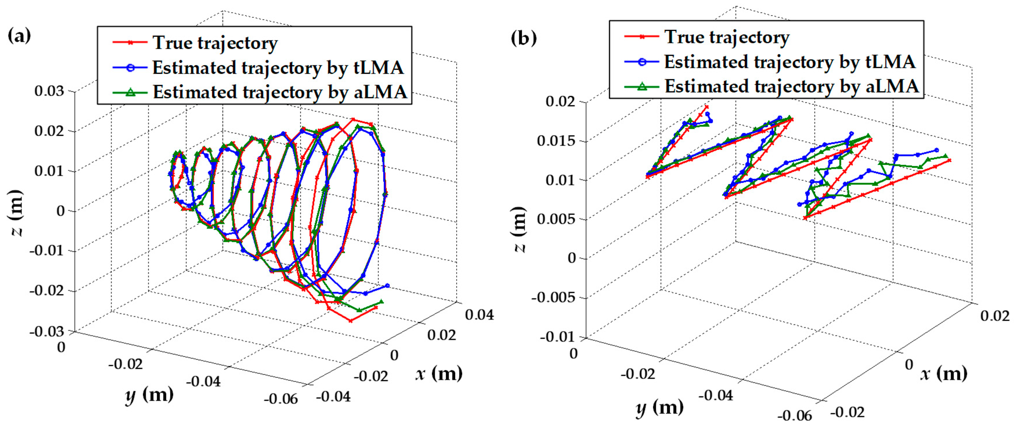
The averaged estimated trajectory of the spiral line and the folding line are presented in Figure 9, which gives an intuitive comparison of the localization results between tLMA and aLMA. The detailed information is given in Table 4 and Table 5, including the mean processing time T and the localization error e of the above three types of methods.
In the spiral line tracking, the mean localization error e for tLMA, ttLMA, and aLMA is 2.4 mm, 1.7 mm, and 1.1 mm, respectively, implying that an improvement of about 54.2% can be brought by the aLMA proposed in this paper with a sacrifice of time about 14.3% increase. Although the improvement brought by ttLMA is 29.2%, 22.4% more time will be required. The improvement in localization accuracy between aLMA and ttLMA is 35.3%, verifying the effect brought by adaptive initialization in aLMA.
In the folding line tracking, the mean localization error e for all three kinds of methods is larger than that in the spiral line tracking. The main reason for this is that the distance between the folding line trajectory and the sensor array is further than that of the spiral trajectory. The improvement of the localization accuracy in the folding line tracking brought by aLMA is 37.1% with the sacrifice of time increasing by about 58.4%, compared to a 20.0% improvement in localization accuracy with the sacrifice of time increasing by about 74.2% using ttLMA. It can be seen from the localization results in Figure 9 and Table 4 and Table 5 that the proposed TCI can realize magnetic localization with a mean accuracy of 1.65 mm within 65.7 ms.
5. Conclusions
In this research, we propose a TCI system utilizing a combined T-type PM localized by an adaptive LM algorithm for potential communications between individuals with severe disabilities and the smart environment. The tongue motion, which has less dependence on initializations and more accuracy in localization, can be derived by the proposed adaptive LM algorithm from the improved magnetic field distribution brought by the attached combined T-type PM. A compressive sensing system calibration method has been developed to figure out the bias in the combined T-type PM and sensing axis. Bench-top experiments based on a high-precision 3D translation platform were carried out to assess the feasibility of the proposed TCI system in magnetic localization accuracy and efficiency. A mean localization accuracy of 1.65 mm within 65.7 ms was achieved. The proof-of-concept prototype TCI creates a basis for application in high-precision interactions. It is known that wearable human–machine interfaces need to be of good portability and compactness, including wireless signal transmission and low-power supply. In the future, efforts in developing standalone TCI and evaluations of the proposed TCI system on the human body in smart infrastructure will be performed.
Author Contributions
H.-M.S. and G.Y. contributed to provide the conceptualization and methodology to this research; H.-M.S., Y.Y. and C.L. designed and performed the experiments; D.G. performed the simulation; H.-M.S. wrote the paper; G.Y. revised the paper.
Funding
This research was funded by the National Natural Science Foundation of China, grant number 51605291.
Conflicts of Interest
The authors declare no conflict of interest.
References
- Zhang, B.; Luo, Y.; Ma, L.; Gao, L.; Li, Y.; Xue, Q.; Yang, H.; Cui, Z. 3D bioprinting: An emerging technology full of opportunities and challenges. Bio-Des. Manuf. 2018, 1, 2–13. [Google Scholar] [CrossRef]
- Yang, Y.; Li, Y.; Chen, Y. Principles and methods for stiffness modulation in soft robot design and development. Bio-Des. Manuf. 2018, 1, 14–25. [Google Scholar] [CrossRef] [Green Version]
- Rashid, Z.; Melià-Seguí, J.; Pous, R.; Peig, E. Using augmented reality and internet of things to improve accessibility of people with motor disabilities in the context of smart cities. Future Gener. Comput. Syst. 2016, 76, 248–261. [Google Scholar] [CrossRef]
- Jafari, A.; Buswell, N.; Ghovanloo, M.; Mohsenin, T. A low-power wearable stand-alone tongue drive system for people with severe disabilities. IEEE Trans. Biomed. Circuits Syst. 2018, 12, 58–67. [Google Scholar] [CrossRef] [PubMed]
- Anaelis, S.; Malek, A.; Mercedes, C.; Melvin, A.; Armando, B. Adaptive eye-gaze tracking using neural-network-based user profiles to assist people with motor disability. J. Rehabil. Res. Dev. 2008, 45, 801–817. [Google Scholar] [CrossRef]
- Postelnicu, C.C.; Girbacia, F.; Talaba, D. EOG-based visual navigation interface development. Expert Syst. Appl. 2012, 39, 10857–10866. [Google Scholar] [CrossRef]
- Williams, M.R.; Kirsch, R.F. Evaluation of head orientation and neck muscle EMG signals as command inputs to a human–computer interface for individuals with high tetraplegia. IEEE Trans. Neural Syst. Rehabil. Eng. 2008, 16, 485–496. [Google Scholar] [CrossRef]
- Paul, G.M.; Cao, F.; Torah, R.; Yang, K.; Beeby, S. A smart textile based facial EMG and EOG computer interface. IEEE Sens. J. 2014, 14, 393–400. [Google Scholar] [CrossRef]
- Fukuma, R.; Yanagisawa, T.; Saitoh, Y.; Hosomi, K.; Kishima, H.; Shimizu, T.; Sugata, H.; Yokoi, H.; Hirata, M.; Kamitani, Y.; et al. Real-Time Control of a Neuroprosthetic Hand by Magnetoencephalographic Signals from Paralysed Patients. Sci. Rep. 2016, 6, 21781. [Google Scholar] [CrossRef]
- Hochberg, L.R.; Bacher, D.; Jarosiewicz, B.; Masse, N.Y.; Simeral, J.D.; Vogel, J.; Haddadin, S.; Liu, J.; Cash, S.S.; van der Smagt, P.; et al. Reach and grasp by people with tetraplegia using a neurally controlled robotic arm. Nature 2012, 485, 372–375. [Google Scholar] [CrossRef] [Green Version]
- Carabez, E.; Sugi, M.; Nambu, I.; Wada, Y. Identifying single trial event-related potentials in an earphone-based auditory brain-computer interface. Appl. Sci. 2017, 7, 1197. [Google Scholar] [CrossRef]
- Shen, H.M.; Hu, L.; Lee, K.M.; Fu, X. Multi-motion robots control based on bioelectric signals from single-channel dry electrode. Proc. Inst. Mech. Eng. H 2015, 229, 124–136. [Google Scholar] [CrossRef] [PubMed]
- Caltenco, H.A.; Breidegard, B.; Struijk, L.N. On the tip of the tongue: Learning typing and pointing with an intra-oral computer interface. Disabil. Rehabil. Assist. Technol. 2014, 9, 307–317. [Google Scholar] [CrossRef] [PubMed]
- Nakatani, S.; Araki, N.; Konishi, Y. Tongue-motion classification using intraoral electromyography for a tongue-computer interface. In Proceedings of the IEEE International Conference on Systems Man and Cybernetics Conference Proceedings, City University of Hong Kong, Hong Kong, China, 9–12 October 2015; pp. 2349–2353. [Google Scholar]
- Takahashi, J.; Suezawa, S.; Hasegawa, Y.; Sankai, Y. Tongue motion-based operation of support system for paralyzed patients. In Proceedings of the IEEE International Conference on Rehabilitation Robotics, ETH Zurich, Zurich, Switzerland, 27 June–1 July 2011. [Google Scholar]
- Choi, C.; Micera, S.; Carpaneto, J.; Kim, J. Development and quantitative performance evaluation of a noninvasive EMG computer interface. IEEE Trans. Bio-Med. Eng. 2009, 56, 188–191. [Google Scholar] [CrossRef] [PubMed]
- Vaidyanathan, R.; Chung, B.; Gupta, L.; Kook, H.; Kota, S.; West, J.D. Tongue-movement communication and control concept for hands-free human–machine interfaces. IEEE Trans. Syst. Man Cybern. Part A Syst. Hum. 2007, 37, 533–546. [Google Scholar] [CrossRef]
- Mamun, K.A.; Mace, M.; Gupta, L.; Verschuur, C.A.; Lutman, M.E.; Stokes, M.; Vaidyanathan, R.; Wang, S.Y. Robust real-time identification of tongue movement commands from interferences. Neurocomputing 2011, 80, 83–92. [Google Scholar] [CrossRef]
- Nam, Y.; Koo, B.; Cichocki, A.; Choi, S. Glossokinetic potentials for a tongue-machine interface: How can we trace tongue movements with electrodes? Syst. Man Cybern. Mag. 2016, 2. [Google Scholar] [CrossRef]
- Rakibet, O.O.; Horne, R.J.; Kelly, S.W.; Batchelor, J.C. Passive wireless tags for tongue controlled assistive technology interfaces. Healthc. Technol. Lett. 2016, 3. [Google Scholar] [CrossRef]
- Struijk, L.N.S.A.; Bentsen, B.; Gaihede, M.; Lontis, E.R. Error-free text typing performance of an inductive intra-oral tongue computer interface for severely disabled individuals. IEEE Trans. Neural Syst. Rehabil. Eng. 2017, 25, 2094–2104. [Google Scholar] [CrossRef]
- Huo, X.; Park, H.; Kim, J.; Ghovanloo, M. A dual-mode human computer interface combining speech and tongue motion for people with severe disabilities. IEEE Trans. Neural Syst. Rehabil. Eng. 2013, 21, 979–991. [Google Scholar] [CrossRef]
- Shen, H.M.; Hu, L.; Qin, L.H.; Fu, X. Real-time orientation-invariant magnetic localization and sensor calibration based on closed-form models. IEEE Magn. Lett. 2015, 6, 1–4. [Google Scholar] [CrossRef]
- Park, H.; Ghovanloo, M. An arch-shaped intraoral tongue drive system with built-in tongue-computer interfacing SoC. Sensors 2014, 14, 21565–21587. [Google Scholar] [CrossRef] [PubMed]
- Huo, X.; Johnson-Long, A.N.; Ghovanloo, M.; Shinohara, M. Motor performance of tongue with a computer-integrated system under different levels of background physical exertion. Ergonomics 2013, 56, 1733–1744. [Google Scholar] [CrossRef] [PubMed] [Green Version]
- Huo, X.L.; Wang, J.; Ghovanloo, M. A Magneto-Inductive Sensor Based Wireless Tongue-Computer Interface. IEEE Trans. Bio-Med. Eng. 2008, 16, 497–504. [Google Scholar] [CrossRef] [Green Version]
- Huo, X.L.; Ghovanloo, M. Evaluation of a wireless wearable tongue–computer interface by individuals with high-level spinal cord injuries. J. Neural Eng. 2010, 7. [Google Scholar] [CrossRef] [PubMed]
- Kim, J.; Park, H.; Bruce, J.; Rowles, D.; Holbrook, J.; Nardone, B. Assessment of the tongue-drive system using a computer, a smartphone, and a powered-wheelchair by people with tetraplegia. IEEE Trans. Neural Syst. Rehabil. Eng. 2016, 24, 68–78. [Google Scholar] [CrossRef] [PubMed]
- Huo, X.L.; Ghovanloo, M. Using Unconstrained Tongue Motion as an Alternative Control Mechanism for Wheeled Mobility. IEEE Trans. Bio-Med. Eng. 2009, 56, 1719–1726. [Google Scholar] [CrossRef]
- Farajidavar, A.; Block, J.M.; Ghovanloo, M. A comprehensive method for magnetic sensor calibration: A precise system for 3-D tracking of the tongue movements. Conf. Proc. IEEE Eng. Med. Biol. Soc. 2012, 4, 1153–1156. [Google Scholar] [CrossRef]
- Hu, C.; Meng, M.Q.H.; Mandal, M. A linear algorithm for tracing magnet position and orientation by using three-axis magnetic sensors. IEEE Trans. Magn. 2007, 43, 4096–4101. [Google Scholar] [CrossRef]
- Song, S.; Li, B.; Qiao, W.; Hu, C.; Ren, H.; Yu, H.; Zhang, Q.; Meng, M.Q.H.; Xu, G. 6-D magnetic and orientation method for an annular magnet based on a closed-form analytical model. IEEE Trans. Magn. 2014, 50, 5000411. [Google Scholar] [CrossRef]
- Lim, J.; Lee, K.M. Distributed multilevel current models for design analysis of electromagnetic actuators. IEEE-ASME Trans. Mech. 2015, 20, 2413–2424. [Google Scholar] [CrossRef]
- Ranganathan, A. The Levenberg-Marquardt Algorithm; Honda Research Institute: Mountain View, CA, USA, 2004. [Google Scholar]
Figure 1.
The tongue–computer interface (TCI) system. (a) The system architecture of the TCI using T-type permanent magnet (PM) marker; (b) Block diagram illustrating the signal procedure.
Figure 1.
The tongue–computer interface (TCI) system. (a) The system architecture of the TCI using T-type permanent magnet (PM) marker; (b) Block diagram illustrating the signal procedure.


Figure 2.
Scheme illustrates the localization x–y–z coordinate system with T-type PM modeled as magnetic dipoles; xs–ys–zs coordinate is parallel with the global Cartesian coordinate x–y–z, with an rp translation to present the orientation vector m (θ, φ) of the tracked point; the xmv–ymv–zmv coordinate in the zoom circle is local system of the vertical magnet PMv to illustrate the deviation mv (θmv, φmv) of the dipole moment from its geometric axis.
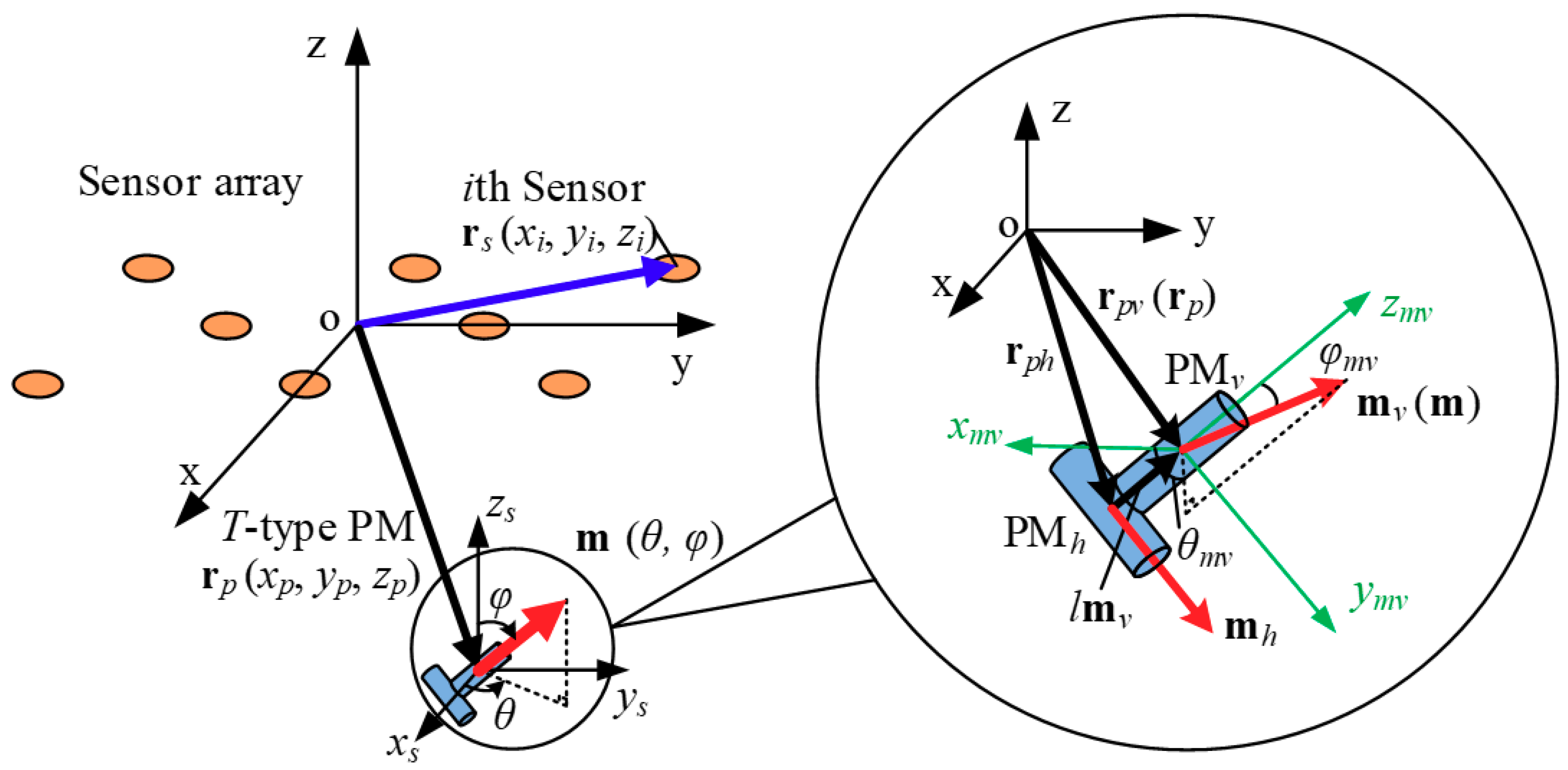
Figure 3.
Design of the adaptive Levenberg–Marquardt algorithm (aLMA).
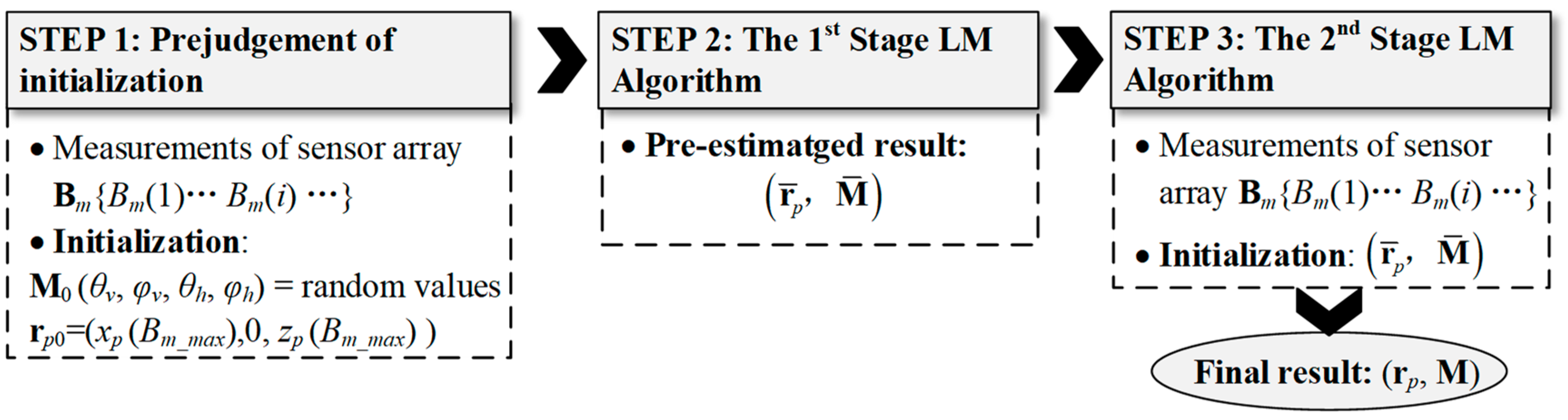
Figure 4.
Experimental setup.

Figure 5.
The custom-made graphical user interface (GUI) constructed based on Labview (NI, Austin, TX, USA) and MATLAB (Mathworks, Natick, MA, USA).
Figure 5.
The custom-made graphical user interface (GUI) constructed based on Labview (NI, Austin, TX, USA) and MATLAB (Mathworks, Natick, MA, USA).
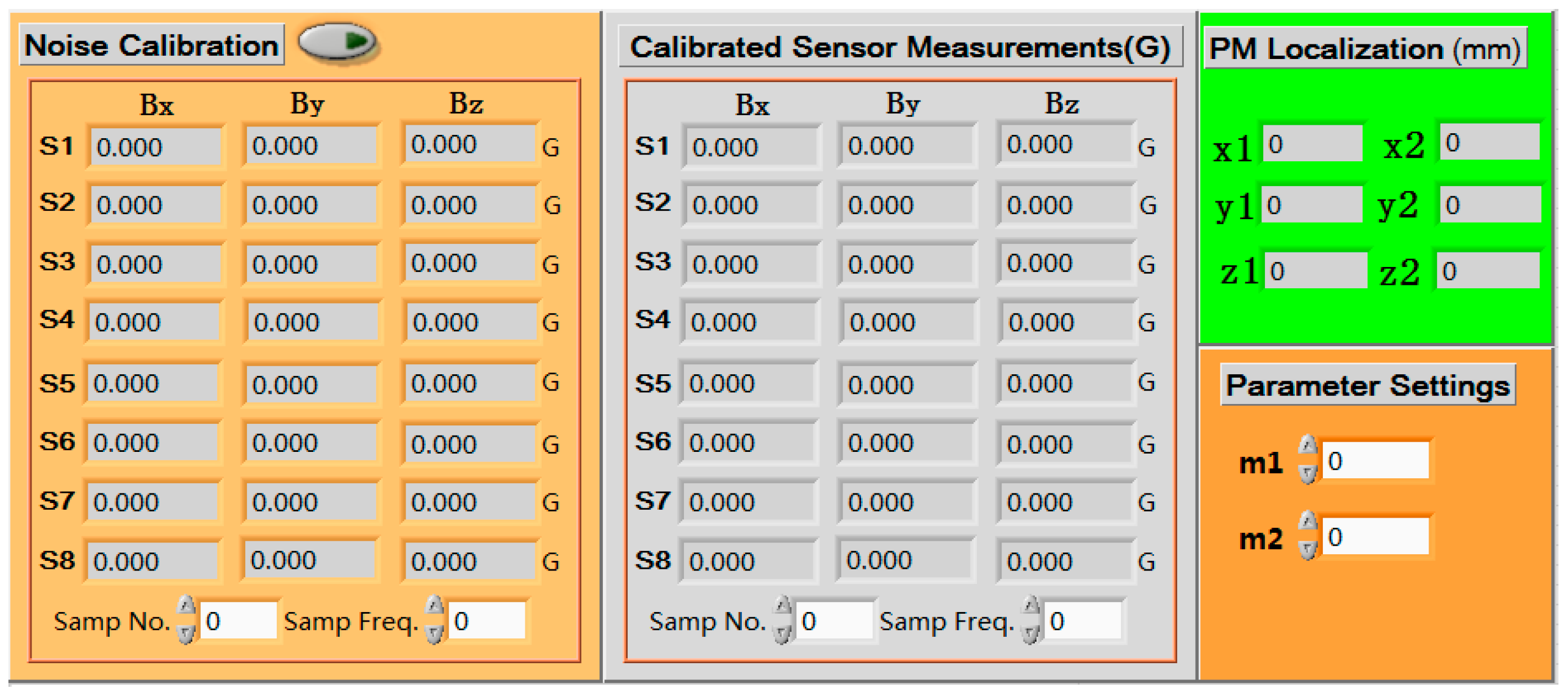
Figure 6.
The target trajectories within a 3 × 3 × 6 cm3 cube. (a) 100 samples on a spiral line; (b) 60 samples on a folding line.
Figure 6.
The target trajectories within a 3 × 3 × 6 cm3 cube. (a) 100 samples on a spiral line; (b) 60 samples on a folding line.
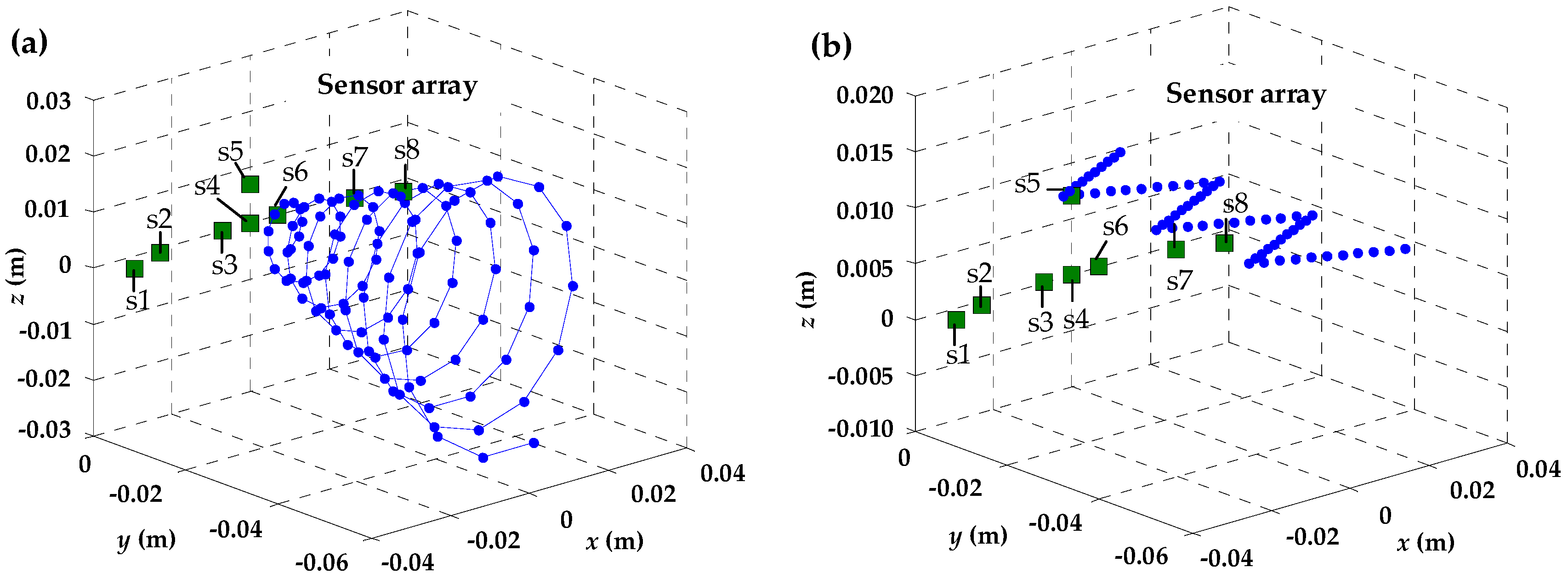
Figure 7.
Comparisons of the magnitude distributions of magnetic fields derived from the combined T-type PM and both of its component magnets. (a) Arrangement illustration of the T-type PM and analyzed magnetic field distribution; (b) B derived from the combined T-type PM; (c) B derived from the magnet PMh; (d) B derived from the magnet PMv.
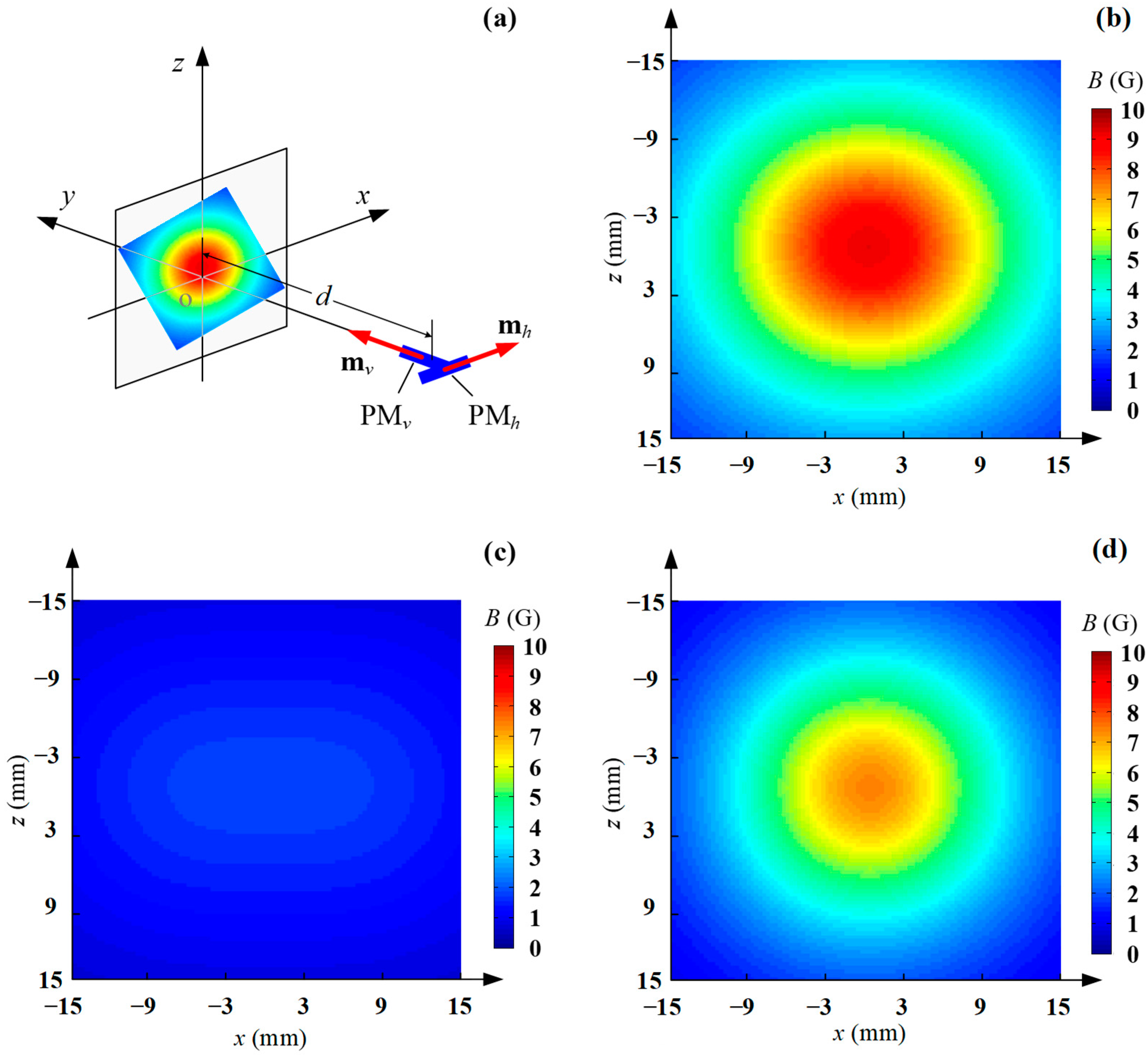
Figure 8.
Measurements of the magnetic field magnitude Bv and Bh derived from different PM by sensors distributed on the sensor array edge and center. (a) The magnetic field magnitude measured by sensor S1 on the sensor array edge of the spiral line trajectory; (b) The magnetic field magnitude measured by sensor S4 on the sensor array center of the spiral line trajectory; (c) The magnetic field magnitude measured by sensor S8 on the sensor array edge of the spiral line trajectory; (d) The magnetic field magnitude measured by sensor S1 on the sensor array edge of the folding line trajectory; (e) The magnetic field magnitude measured by sensor S4 on the sensor array center of the folding line trajectory; (f) The magnetic field magnitude measured by sensor S8 on the sensor array edge of the folding line trajectory.
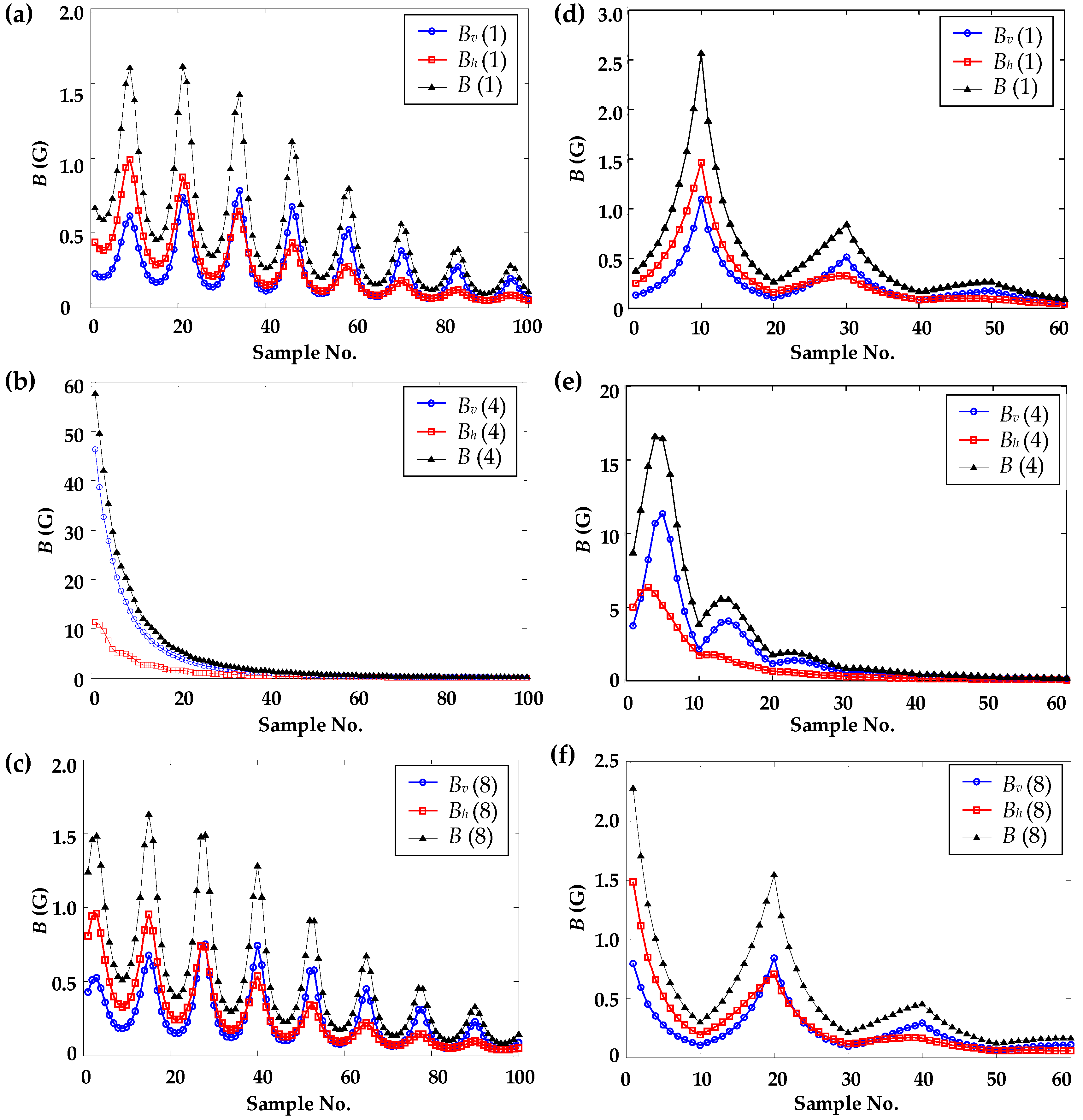
Figure 9.
Comparison of the trajectories estimated by a traditional Levenberg–Marquardt algorithm (tLMA) and a twice-traditional Levenberg–Marquardt algorithm (aLMA) of the proposed TCI system.
Figure 9.
Comparison of the trajectories estimated by a traditional Levenberg–Marquardt algorithm (tLMA) and a twice-traditional Levenberg–Marquardt algorithm (aLMA) of the proposed TCI system.


Table 1.
Experimental setups. AMR: anisotropic magnetoresistive.
| Components | Property | Manufacture |
|---|---|---|
| T-type PM | Two NdFe-B magnet; Axially magnetized; Φ = 1.56 mm, 2l = 6.48 mm; Br = 0.1430 T | MISUMI, Tokyo, Japan |
| AMR sensor | Eight three-axis HMC5983; Resolution: 0.227 μT; Maximum output rate: 220 Hz Range: ±0.4 mT | Honeywell, Plymouth, MN, USA |
| I2C–USB adapter | VTG200A; 12-bit; | Viewtool, Shenzhen, China |
| Gauss meter | Model-421; resolution: 0.1 μT | Lakeshore, Westerville, OH, USA |
| 3D translation platform | Resolution: 10 μm | MITSUBISHI, Tokyo, Japan |
Table 2.
Calibration results for the PM marker.
| m (A·m2) | (φm, θm) (°) | e|B| (%) at P(0, 0, 0.025) (m) | |
| PMv | 0.0125 ± 0.0001 | (1.71, 74.18) | 0.33 |
| PMh | 0.0123 ± 0.0005 | (0.97, 137.53) | 0.21 |
Table 3.
Sensing axis calibration results.
Table 4.
The mean processing time T and localization error e in spiral line tracking.
| tLMA | ttLMA | aLMA | |
|---|---|---|---|
| T (ms) | 62.3 | 85.2 | 71.2 |
| e (mm) | 2.4 | 1.7 | 1.1 |
Table 5.
The mean processing time T and localization error e in folding line tracking.
| tLMA | ttLMA | aLMA | |
|---|---|---|---|
| T (ms) | 38.0 | 66.2 | 60.2 |
| e (mm) | 3.5 | 2.8 | 2.2 |
© 2018 by the authors. Licensee MDPI, Basel, Switzerland. This article is an open access article distributed under the terms and conditions of the Creative Commons Attribution (CC BY) license (http://creativecommons.org/licenses/by/4.0/).
Share and Cite
MDPI and ACS Style
Shen, H.-M.; Yue, Y.; Lian, C.; Ge, D.; Yang, G. Tongue–Computer Interface Prototype Design Based on T-Type Magnet Localization for Smart Environment Control. Appl. Sci. 2018, 8, 2498. https://doi.org/10.3390/app8122498
AMA Style
Shen H-M, Yue Y, Lian C, Ge D, Yang G. Tongue–Computer Interface Prototype Design Based on T-Type Magnet Localization for Smart Environment Control. Applied Sciences. 2018; 8(12):2498. https://doi.org/10.3390/app8122498
Chicago/Turabian StyleShen, Hui-Min, Yang Yue, Chong Lian, Di Ge, and Geng Yang. 2018. "Tongue–Computer Interface Prototype Design Based on T-Type Magnet Localization for Smart Environment Control" Applied Sciences 8, no. 12: 2498. https://doi.org/10.3390/app8122498
Note that from the first issue of 2016, this journal uses article numbers instead of page numbers. See further details here.