Characterizing Situations of Dock Overload in Bicycle Sharing Stations
by
 , ,
, ,
Luca Cagliero
1,*, 
Tania Cerquitelli
1,
Silvia Chiusano
2,
Paolo Garza
1 ,
,
Giuseppe Ricupero
1 and
Elena Baralis
1 1
Dipartimento di Automatica e Informatica, Politecnico di Torino, Corso Duca degli Abruzzi, 24, 10129 Torino, Italy
2
Dipartimento Interateneo di Scienze, Progetto e Politiche del Territorio, Politecnico di Torino, Viale Pier Andrea Mattioli, 39, 10125 Torino, Italy
*
Author to whom correspondence should be addressed.
Appl. Sci. 2018, 8(12), 2521; https://doi.org/10.3390/app8122521
Submission received: 10 October 2018
/
Revised: 25 November 2018
/
Accepted: 3 December 2018
/
Published: 6 December 2018
(This article belongs to the Special Issue IoT for Smart Cities)
Abstract
:Bicycle sharing systems are becoming increasingly popular in cities around the world as they are an inexpensive and sustainable means of transportation. Promoting the use of these systems substantially improves the quality of life in cities by reducing pollutant emissions and traffic congestion. In these systems, bikes are made available for shared use to individuals on a short-term basis. They allow people to borrow a bike in one dock and return it to any other station with free docks belonging to the same system. The occupancy level of the stations can be constantly monitored. However, to achieve a satisfactory user experience, all the stations in the system must be neither overloaded nor empty when the user needs to access the station. The aim of this paper is to analyze occupancy level data acquired from real systems to determine situations of dock overload in multiple stations which could lead to service disruption. The proposed methodology relies on a pattern mining approach. A new pattern type called Occupancy Monitoring Pattern is proposed here to detect situations of dock overload in multiple stations. Since stations are geo-referenced and their occupancy levels are periodically monitored, occupancy patterns can be filtered and evaluated by taking into consideration both the spatial and temporal correlation of the acquired measurements. The results achieved on real data highlight the potential of the proposed methodology in supporting domain experts in their maintenance activities, such as periodic re-balancing of the occupancy levels of the stations, as well as in improving user experience by suggesting alternative stations in the nearby area.
1. Introduction
In recent years, municipalities have fostered alternative ways of public transportation in order to reduce pollution and traffic congestion [1,2,3,4,5]. Bicycle sharing systems [6,7] are a notable example of eco-friendly transportation systems, where citizens can rent bicycles on a short-term basis. Bikes are retrieved from stations spread throughout the city and each station has a maximum capacity as it is equipped with a fixed number of docks. Citizens can rent a bicycle parked at any station and return it to any other station with free docks. However, to achieve a satisfactory user experience, system managers should carefully monitor the level of occupancy of the stations. For example, if a station is frequently overloaded at peak hours, then a re-balancing action should be scheduled in order to move some of the parked bicycles to any station located in the neighborhood. In case the problem is more severe, managers may decide to expand the station to fit the increasing demand. Stations are geo-referenced and equipped with sensors to constantly monitor their level of occupancy. Each station tracks the occupancy levels of its docks, thus providing geo-referenced time series data. These data acquired from stations can be collected and stored in a unique repository and analyzed by means of machine learning and data analytics techniques. Automating the process of analysis of the acquired occupancy level data is particularly appealing to computerize the planning of maintenance activities as well as giving targeted recommendations to the system users [8].
This work presents a novel exploratory data-driven methodology, named Bike Station OvErLoad AnaLyzer (BELL), which analyzes the occupancy levels of the stations of a bicycle sharing system. The aim is to identify situations of dock overload in multiple stations which could lead to either service disruption or low customer satisfaction. For example, when all the docks in a station are occupied, users have to move to a nearby station to park their bike. By gathering insightful information regarding occupancy levels of multiple stations, domain experts can effectively apply targeted actions in order to avoid and/or limit the unpleasant situations described above. For instance, the mobile application of the system may recommend alternative nearby stations with free docks. Furthermore, the maintenance service may re-balance the number of bikes in each station thus avoiding overloaded conditions. For this reason, the proposed methodology would allow us to improve user experience in using the service.
In the BELL methodology occupancy level data acquired from the geo-referenced stations are analyzed to discover a new type of pattern, called Occupancy Monitoring Pattern (OMP). OMPs describe in a concise way situations of imbalance in the occupancy levels of spatially correlated stations. Specifically, OMPs model two complementary dock overload situations: (i) Situations in which a set of stations are overloaded in an alternate fashion (hereafter denoted as intermittent situations); and (ii) Situations in which the docks of a set of stations are frequently overloaded at the same time (hereafter denoted as critical situations). To consider the spatial correlation between the occupancy level of different stations, spatial constraints can be enforced to represent groups of nearby stations in OMPs (i.e., stations within a limited geographical distance).
Intermittent and critical situations are treated separately because they cause disservices with varying degrees of severity for end users. Specifically, intermittent situations indicate an imbalance in station usage which could be addressed by proposing alternative nearby stations to end users or by periodically repositioning the bicycles in the neighborhood. Conversely, critical situations indicate that a given area is temporarily inaccessible for parking bikes because all the stations in the area are in a dock overload situation. The latter (more severe) situation can be addressed, for example, by increasing the number of available docks in the stations, or by moving bikes to the not fully occupied stations located in other city areas.
The generated OMPs are explored to discover significant intermittent and critical situations. The exploration is driven by two ad hoc quality indices introduced in this study, namely the intermittence and the criticality indices, which allow domain experts to focus on the most severe warnings.
The use of the BELL methodology allows the municipality to improve dwellers’ experience. OMPs permit a spatio-temporal exploration of critical and intermittent situations. Since stations are geo-referenced, OMPs display the city areas where disservices are likely to occur. Moreover, since OMPs can be related to specific time periods, they allow experts to identify when these disservices are likely to occur.
The proposed BELL methodology generates OMPs by means of a two-step itemset-based process, which is driven by the two quality indices proposed in this study. BELL has been thoroughly evaluated using real datasets acquired from the bicycle sharing systems of two important cities, i.e., Barcelona (Spain) and New York (USA). The experimental results demonstrated the effectiveness of BELL in identifying useful knowledge regarding the spatio-temporal distribution of possible service disruptions for end users of bicycle sharing systems. We envisioned possible scenarios of usage of the extracted patterns aimed at supporting maintenance activities and improving user experience.
This paper is organized as follows. Section 2 overviews the literature. Section 3 presents and thoroughly describes the proposed approach. Section 4 experimentally evaluates the performance of our implementation of the BELL methodology on data acquired in real urban environments. Section 5 discusses the policy implications of the presented results and presents future developments of this work. Section 6 draws conclusions.
2. Literature Review
The analysis of urban data related to bicycle sharing systems has already been addressed in previous studies. Specifically, in this field, the main branches of research can be categorized as follows: (i) Grouping stations based on their usage profile [9,10,11,12], (ii) Predicting future station occupancy levels [13,14,15,16,17], and (iii) Repositioning bicycles between the stations [18,19,20,21,22,23].
Branch (i) focuses on identifying groups of stations with different usage profiles by applying unsupervised machine learning techniques (e.g., clustering [9]). To characterize station usage, temporal features [9], spatial features [10], or a mix of the above [11] are considered. Instead of partitioning the set of stations into disjointed groups according to their common usage pattern, the methodology proposed in this study focuses on locating sets of nearby stations showing a critical or alternate usage profile (e.g., a station is overloaded, whereas the nearby station is almost empty). To the best of our knowledge, the information provided by OMPs, which is the core of the BELL methodology, cannot be obtained by any of the existing approaches.
Branch (ii) aims at forecasting the occupancy level of a station in the near future (i.e., with a time horizon between 30 min and 2 h ahead) by applying supervised machine learning techniques (e.g., regression [13,14,15,24], classification [16,17]). Based on these predictions, a recommender system can be integrated into the mobile application of the provider to suggest the stations close to the user-specified point of interest with a sufficient number of free docks/available bicycles. Predictions are based not only on past occupancy levels but also on contextual information (e.g., meteorological data [24]). The main differences between the aforesaid works and the proposed approach are enumerated below: (i) Unlike the aforesaid approaches, this work does not address the problem of forecasting the station occupancy levels using supervised techniques. Conversely, it presents a methodology based on an unsupervised technique. (ii) In the prediction task, the aim is to forecast short-term variations in occupancy level (typically, between 30 min and 2 h ahead). Our work aims at identifying recurrent situations of imbalance in dock occupancy, which policymakers may consider for scheduling medium- and long-term maintenance actions (e.g., re-balance the number of bicycles in the stations, resize the existing stations, place new stations).
Branch (iii) focuses on planning the re-balance of the bicycles in stations according to actual user demands (e.g., more bicycles close to parking areas and business centers or more free docks close to restaurants at lunchtime). The aim is to support providers in improving user experience. For example, in [12], the authors performed a stochastic characterization of demand to design fleet-management strategies dealing with flow asymmetries. The problem is complementary to the one addressed in this paper because detecting dock overload situations could trigger re-balance actions driven by optimization-based strategies such as [18,22,23].
3. Methodology
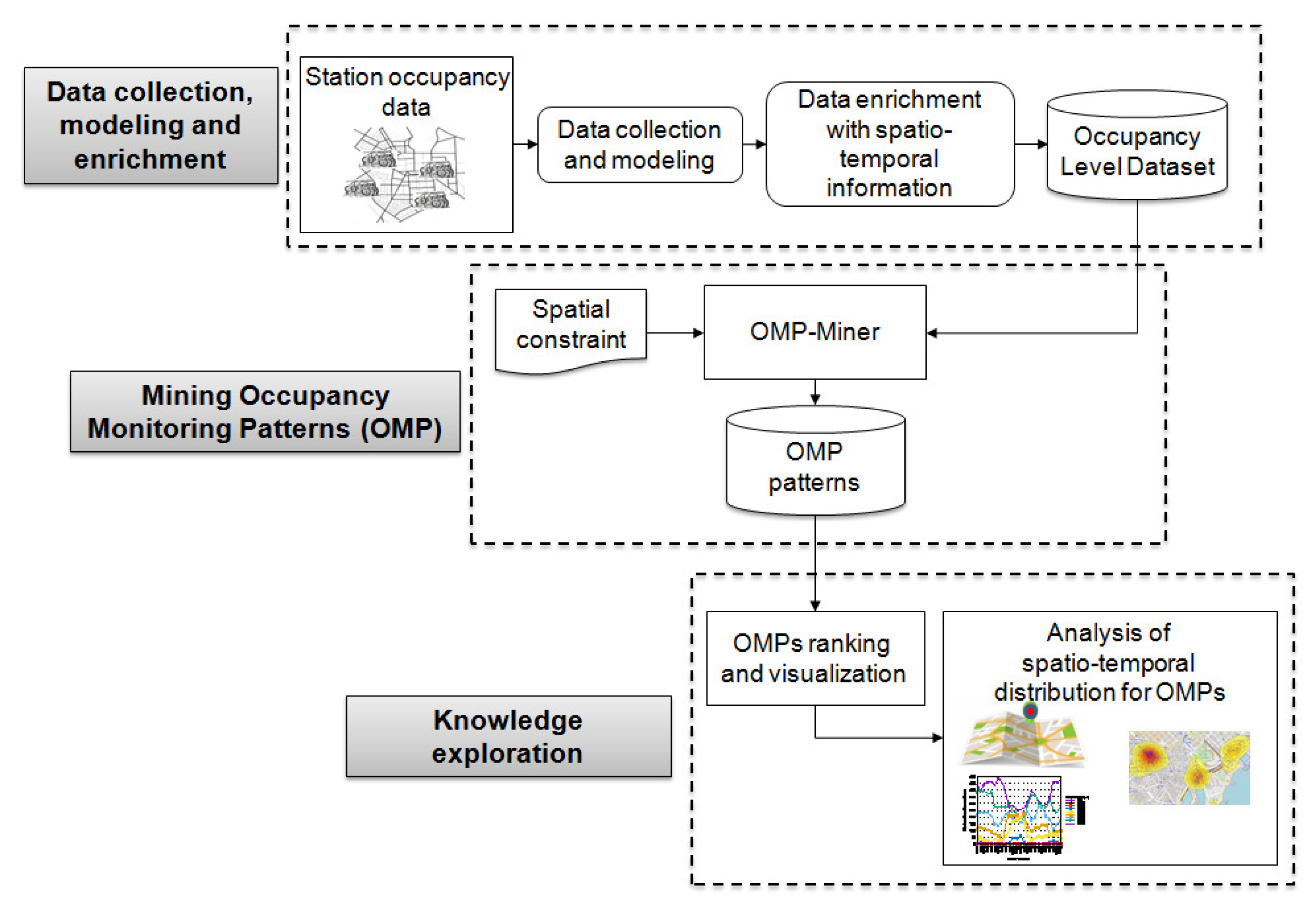
BELL is a new data mining methodology aimed at monitoring the occupancy levels of the stations in a bicycle sharing system. The main architecture blocks, depicted in Figure 1, are (i) Data collection, modeling and enrichment (ii) Mining Occupancy Monitoring Patterns (OMP), which entails discovering OMP patterns from the prepared data, and (iii) Knowledge exploration, which consists of exploring the extracted OMPs to discover actionable knowledge. A more thorough description of each step is given in the following sections. Table A1 summarizes the notation used throughout the sections.
3.1. Data Collection, Modeling and Enrichment
To monitor the usage of the bicycle sharing system, the occupancy levels of all the stations are acquired at different points of time and stored into an Occupancy level dataset. Collected data are then enriched with additional spatial and temporal information needed to support the subsequent data analysis phase.
Data collection and modeling. Given a time window and a set = {, …, } of points of time in , for each station in the system, the number of free parkings at each time is acquired and collected in a unique repository named Occupancy level dataset (). is modeled as a relational dataset [25]. A more formal definition follows.
Definition 1 (Occupancy level dataset).
Let be an arbitrary time window and let be a set of sampling time points in . Let be a set of attributes, where each attribute represents a different station in the bicycle sharing system. Let (, ) be an arbitrary pair denoting the occupancy level of station at a given timestamp . The record indicates the occupancy levels of all the stations in at time , i.e., it is a set of pairs {(, )}, . Each record is logically identified by a Record IDentifier (RID). An occupancy level dataset associated with time period is defined as .
Station occupancy values are categorized into two different classes to indicate the occupancy level of the station. Specifically, the measurements indicating the number of free parkings at a station are labeled as follows: (i) Overloaded, if the number of freely available parkings is below a given occupancy threshold full-th, or (ii) Normal, if the number of freely available parkings is equal to or above full-th. The occupancy level threshold full-th is an absolute value specified by the domain expert. Label Overloaded is used to denote stations with a critical occupancy level, such that end users may not find free docks for parking. Instead, label Normal is used to denote station conditions that should not cause a disservice to end users.
Table 1 shows an example of an occupancy level dataset. The dataset stores the occupancy levels of three arbitrary stations (, , ) at seven points of time (–). The dataset contains seven records logically identified with a RID (RID-RID). Each record includes the occupancy levels of the three stations at a given point of time.
Notice that this study will not address the complementary problem of detecting sets of underutilized stations. However, since our proposed methodology is general, it can be straightforwardly adapted to deal with this complementary problem.
Data enrichment with temporal information. The analysis of station occupancy levels at different time granularities allows system managers to investigate how overload conditions evolve over time, and to identify overload conditions that frequently happen in specific time periods. To support this analysis, the occupancy level data have been enriched with a temporal information with a coarser granularity.
In dataset , each record includes the occupancy levels of all the stations acquired at a different point of time . Each record is enriched with an additional attribute specifying the corresponding time period for the point of time . In the example dataset in Table 1, records are associated with three different time periods denoted as , , and . The granularity of the time period can be defined based on the target analysis. For example, hourly or daily time slots can be selected as reference time periods to monitor dock overload situations during the day.
Data enrichment with spatial information. To detect dock overload situations restricted to a given area, we enrich occupancy level data with spatial information. Since all the stations in the system are geo-referenced, the geographical coordinates of all the stations in the system is collected. This information is used in our approach to compute the pairwise distances between stations.
3.2. Mining Occupancy Monitoring Patterns
To automatically detect recurrent dock overload conditions in multiple stations, we propose a new type of pattern, anmed Occupancy Monitoring Pattern (OMP). OMPs represent sets of stations showing a dock overload condition which may cause a disservice to the end users of the bicycle sharing system. An algorithm is proposed in this study to efficiently extract all the OMPs of nearby stations and to compute their quality measures from a given occupancy level dataset.
The following sections are organized as follows. The main properties of OMPs are presented in Section 3.2.1. In Section 3.2.2, the OMP mining problem has been addressed as an itemset mining problem, while the proposed algorithm for OMP extraction is described in Section 3.2.3.
3.2.1. OMP Characterization
OMPs allow to detect dock overload conditions in multiple stations. More specifically, OMPs represent the following situations:
- Critical situation. The occupancy levels of a group of stations are frequently overloaded at the same time. In this case, simultaneously, all the stations in the group are fully occupied.
- Intermittent situation. The occupancy levels of a group of stations are frequently overloaded in an alternate fashion. At a given point of time, some stations are fully occupied whereas the other ones are almost empty. At another point of time, the occupancy level of the same stations could be the opposite.
To consider only sets of nearby stations, i.e., stations with a limited geographical distance in the city area, a spatial constraint can be enforced. Enforcing such a constraint implies that the OMPs consist of stations with maximal geographical distance below a given (analyst-provided) threshold.
Critical situations are potentially harmful because, when all the stations in the group are overloaded, users cannot return the rented bicycles. In particular, the discovery of a group of overloaded stations implies that a specific city area is temporarily unaccessible. To quantitatively evaluate the severity of this issue, we introduced a measure denoted as criticality. This measure counts the number of recorded timestamps (i.e., the number of dataset records) at which all the stations of the considered OMP have a critical level of occupancy.
Intermittent situations are potentially harmful as well because the stations in the group are overloaded in an alternate fashion. While considering nearby stations, some free docks are available in the corresponding area, but a potential service disruption may occur when a user arrives at an overloaded station. Still, the user could reach any of the close stations, since some of them are underutilized. To quantitatively estimate the severity of an intermittent situation, we introduced the intermittence measure. Intermittence counts the number of points of time at which at least one station (but not all of them) of the considered OMP has an occupancy level above a given threshold. The higher the intermittence, the more severe the imbalance situation.
More formal definitions of the OMP and its quality measures follow.
Definition 2 (Occupancy Monitoring Pattern).
Let be an occupancy level dataset and let be its attribute set. An Occupancy Monitoring Pattern (OMP) P in is a set of k distinct stations in , i.e., P = {, …, }, .
Definition 3 (Criticality measure).
The criticality of an OMP P in dataset indicates the number of records in for which all the stations in P take value Overloaded. It is defined as the number of in such that the following conditions hold: (i) ; (ii) .
The criticality values of similar OMPs are correlated with each other. Specifically, if an OMP P is a subset of another OMP (i.e., ), then the criticality of P is above or equal to those of . Such a notable property, called anti-monotonicity, will be exploited to efficiently mine OMPs (see Section 3.2.2).
Definition 4 (Intermittence measure).
The intermittence of an OMP P in dataset indicates the number of records in for which at least one station, but not all of them at the same time, takes value Overloaded. It is defined as the number of in for which the following conditions hold: (i) such that and ; (ii) such that and .
Criticality and intermittence values can be normalized by the number of records in . Their normalized values are usually denoted as relative criticality/intermittence values.
Example 1.
P = {, } is an OMP consisting of a couple of stations (i.e., and ). In Table 1, to compute the criticality and intermittence values of P in dataset , we evaluated the occupancy levels of stations and at different timestamps. Since they are overloaded at the same time only in one timestamp (see record with identified RID associated with timestamp ), the relative criticality value of P is (14.28%). In four timestamps (i.e., , , , corresponding to records with RIDs equal to RID, RID, RID, RID), one station is overloaded, whereas the other is normal. Therefore, the relative intermittence value of P is (57.14%).
To analyze how the occupancy level of stations evolves over time as well as detect dock overload situations happening within limited time ranges, the criticality and intermittence measures of an OMP can be reformulated by considering only the records related to a specific time period. This allows us to discover interesting patterns at a finer granularity level. Based on the target application, the time period with a suitable time granularity can be selected for monitoring the usage of stations. Given an OMP P, its criticality and intermittence value in a time period are computed considering only the subset of records with time period equal to .
Definition 5 (Criticality and Intermittence measures in time period TPk).
Let be an arbitrary time period in dataset . Let () be the subset of records in that are associated with timestamps in . The criticality of an OMP P in is defined as the number of in such that the following conditions hold: (i) ; (ii) . The intermittence of an OMP P in is defined as the number of in for which the following conditions hold: (i) such that and ; (ii) such that and .
OMPs can be filtered based on the spatial distance between the corresponding stations. For this purpose, we introduce a spatial constraint maxdist on OMPs. This constraint specifies the maximum geographical distance (denoted maxdist) between stations in each OMP. OMPs satisfying the spatial constraint represent sets of nearby stations showing an overload situation. The higher is maxdist, the larger is the area including stations with critical/intermittent levels of dock occupancy.
Definition 6 (Spatial constraint).
Let be a positive number. An OMP P satisfies the spatial constraint if for every pair of stations , , their geographical distance d() is below maxdist.
Given an OMP P = {, …, } that satisfies the spatial constraint, every subset satisfies it as well. In fact, if for all pairs of stations the condition d() < maxdist is verified, it easily follows that the condition is also verified for all pairs of stations in . Such a property, called an anti-monotonicity property, will be particularly useful for efficiently generating all the OMPs of interest (see Section 3.2.2).
In our implementation of the proposed methodology, geographical distances between stations were approximated with the Euclidean measure [25] thus disregarding the road network, the presence of obstacles, bridges, or underpasses. As discussed in [26], it can be deemed as a justifiable simplification since (i) Cities generally act to maximize the permeability of movement for pedestrians and cyclists, (ii) Network distances for ciclying journeys are not significantly longer than Euclidean distances, especially in the city center. Similar approximations were made in other studies focused on bike and car sharing system data analyses as well (e.g., [21,27]).
3.2.2. Proposed Approach for OMP Mining
The problem of generating OMPs has been addressed as an itemset mining problem. Itemset mining is an exploratory data mining technique which consists of discovering interesting and useful patterns in transactional databases [28]. More specifically, it entails discovering the groups of attribute values that frequently co-occur in the analyzed database. Itemset mining has been applied in various application domains such as market basket analysis, bio-informatics, text mining, product recommendation, and Web clickstream analysis.
To enable the itemset mining process in our target context, the records contained in are tailored to a transactional data format. To this purpose, we first introduce the concept of occupancy item (o-item, in short); next, each record is represented in a transactional data format as a set of o-items.
An o-item represents a dock occupancy measurement acquired within a given time period and associated with a given station. More formally, an o-item is modeled as a triple , where is an arbitrary station, is the occupancy level of station at any timestamp , and is a time period. Note that the exact timestamp at which the measurement was acquired is not explicitly reported in the o-item because the goal is to identify the stations that have acquired critical dock occupancy levels within each time period.
In the transactional dataset , each transaction is logically identified by a Transaction IDentifier (TID). Each record contained in is represented as a transaction in characterized by the same identification value (i.e., a record with RID equal to RID is mapped to a transaction with TID equal to TID).
Example 2.
An occupancy itemset (o-itemset, in short) is a set of o-items (of arbitrary size) such that all the contained o-items correspond to the same time period. The frequency of an o-itemset is the number of transactions including it.
Example 3.
{, } is an o-itemset with frequency equal to 2 in the transactional dataset in Table 2 because it occurs in transactions with TID equal to TID and TID. This o-itemset indicates that stations and were temporarily overloaded in two different measurements acquired in period .
OMPs and their criticality and intermittence values can be derived from the mined o-itemsets. Therefore, our proposed methodology for OMP mining is based on the following two steps. First, o-itemsets are mined. Then, OMPs are generated on top of the mined o-itemsets and their criticality and intermittence values are computed. In the following, the two steps are separately described.
Step 1: O-itemset mining. A set of o-itemsets is extracted from the transactional representation of the occupancy level dataset. Each of the mined o-itemsets satisfies the following conditions. (i) All the contained o-items have the same occupancy level (i.e., all normal or all overloaded); and (ii) All the stations contained in the o-itemset satisfy the spatial constraint maxdist. Thus, for every pair of stations appearing in the o-itemset, their geographical distance is below maxdist.
Condition (i) allows us to extract two different types of o-itemsets: the critical o-itemsets, which include only the o-items with occupancy level overloaded, and the normal o-itemsets, which include only the o-items with occupancy level normal. These o-itemsets combine the stations having all the same occupancy level in a given time period. As discussed below, these two o-itemset types will be useful at the next step to compute the OMP intermittence value. Condition (ii) allows us to filter out the combinations of o-items related to faraway stations. This will allow us to generate only OMPs including nearby stations in Step 2.
Step 2. OMPs generation. The output of Step 1 is processed at Step 2 to generate the set of OMPs. An OMP P is generated from a pair of critical and normal o-itemsets that include (i) the same stations and (ii) the same time period. The frequency values of these two o-itemsets are used to compute the criticality and intermittence values of P.
The OMP generation process is detailed here using an example case. Let us consider a pair of critical (denoted ) and normal (denoted ) o-itemsets, having both the same stations and the same time period. Consider for instance the critical o-itemset = {, } and the normal o-itemset = {, }. Let denote as and their respective frequency in time period in the analyzed dataset. Let P be the OMP generated from these two o-itemsets. The following statements hold:
- (i)
- Pattern P contains all the stations appearing in the critical o-itemset (or equivalently in the normal o-itemset ), i.e., P = {}.
- (ii)
- According to Definition 5, the criticality of pattern P in time period is the number of times all the stations in P are overloaded in . It follows that that criticality of P in period is equal to the number of transactions in including the o-itemset . Thus,
- (iii)
- According to Definition 5, the intermittence of pattern P in a time period is the number of times at least one station in P (but not all stations at the same time) is overloaded in . It follows that the intermittence of P in period is equal to the total frequency of all o-itemsets with the same stations as P, such that at least one station (but not all them at the same time) is overloaded in . For the sake of efficiency, our approach avoids generating all these o-itemsets, but instead it proceeds as follows. Let us denote as the total number of transactions in period in the analyzed dataset. It easily follows that is equal to the sum of the following three terms: the frequency of the critical o-itemset (), the frequency of the normal o-itemset () and the total frequency of all o-itemsets with the same stations as P, such as at least one station (but not all them at the same time) is overloaded at time . Therefore, we compute the intermittence of P in period as
Example 4.
P = {, } is an OMP with criticality equal to 1 and intermittence equal to 2 in time period . These measures are computed based on the frequencies of the critical o-itemset {, } and of the normal o-itemset {, }. The critical o-itemset has frequency equal to 1 being contained in the transaction with TID equal to TID. Thus, the criticality of P is equal to freq_value(critical) = 1. The normal o-itemset has frequency equal to 1 since it is included in the transaction with TID equal to TID (i.e., freq_value(normal) = 1). card_value is equal to 4 because four transactions refer to time period . Based on Equation (2), it follows that the intermittence of P is computed as intermittence = 4 − (1 + 1) = 2. This intermittence value corresponds to the total frequency of the o-itemsets {, } and {, }, respectively contained in the transactions with TIDs equal to TID and TID.
In Section 3.2.3, we describe the algorithm used in the BELL framework to mine the OMPs including nearby stations according to the spatial constraint maxdist as well their criticality and intermittence values.
3.2.3. The OMP-Miner Algorithm
Algorithms 1 and 2 report the pseudo-code of the algorithm we devised to extract OMPs. It consists of the following three main phases:
- Phase 1: Creation of a compact in-memory representation of the occupancy level transactional dataset (Algorithm 1, line 1).
- Phase 2: Mining of all the critical and normal o-itemsets including nearby stations according to the spatial constraint maxdist (Algorithm 1, line 2).
- Phase 3: Generation of the OMPs on top of the mined o-itemsets and computation of their criticality and intermittence levels (Algorithm 1, lines 3–7).
To implement the o-itemset mining phase of the proposed methodology, we exploited an itemset-based approach relying on the state of the art FP-growth algorithm [29]. The main advantage of the FP-growth based approach is the selective generation of the candidate o-itemsets, which prevents the time- and memory-consuming candidate generation phase adopted by the a priori strategy [30].
| Algorithm 1 OMP-Miner(, maxdist, ) |
| Require:: occupancy level dataset in transactional format |
| Require:maxdist: maximum distance between two stations in the same OMP |
| Require:: set of time periods , …, |
| Ensure:: the set of OMPs for each time period in |
| 1: ← FP-tree() {Create the initial FP-tree from } |
| 2: O-ITEMSETMining(, maxdist, ∅) {Recursive projection-based o-itemset mining function} {Generate OMPs on top of the mined o-itemsets in } |
| 3: : normal o-itemsets in |
| 4: : critical o-itemsets in |
| 5: : Hash map with keys storing the criticality values of each normal o-itemset ∈ for each period |
| 6: card_value[]: vector storing in the k-th element the number of transactions in associated with period |
| 7: = ComputeOMPintermittence(,card_value) |
| 8: return |
Phase 1 entails storing the measurements reported in the transactional representation of the original dataset into a compact tree-based structure. To accomplish this task, we exploit the prefix-tree data structure adopted by FP-Growth, namely the FP-tree, to store the transactional dataset .
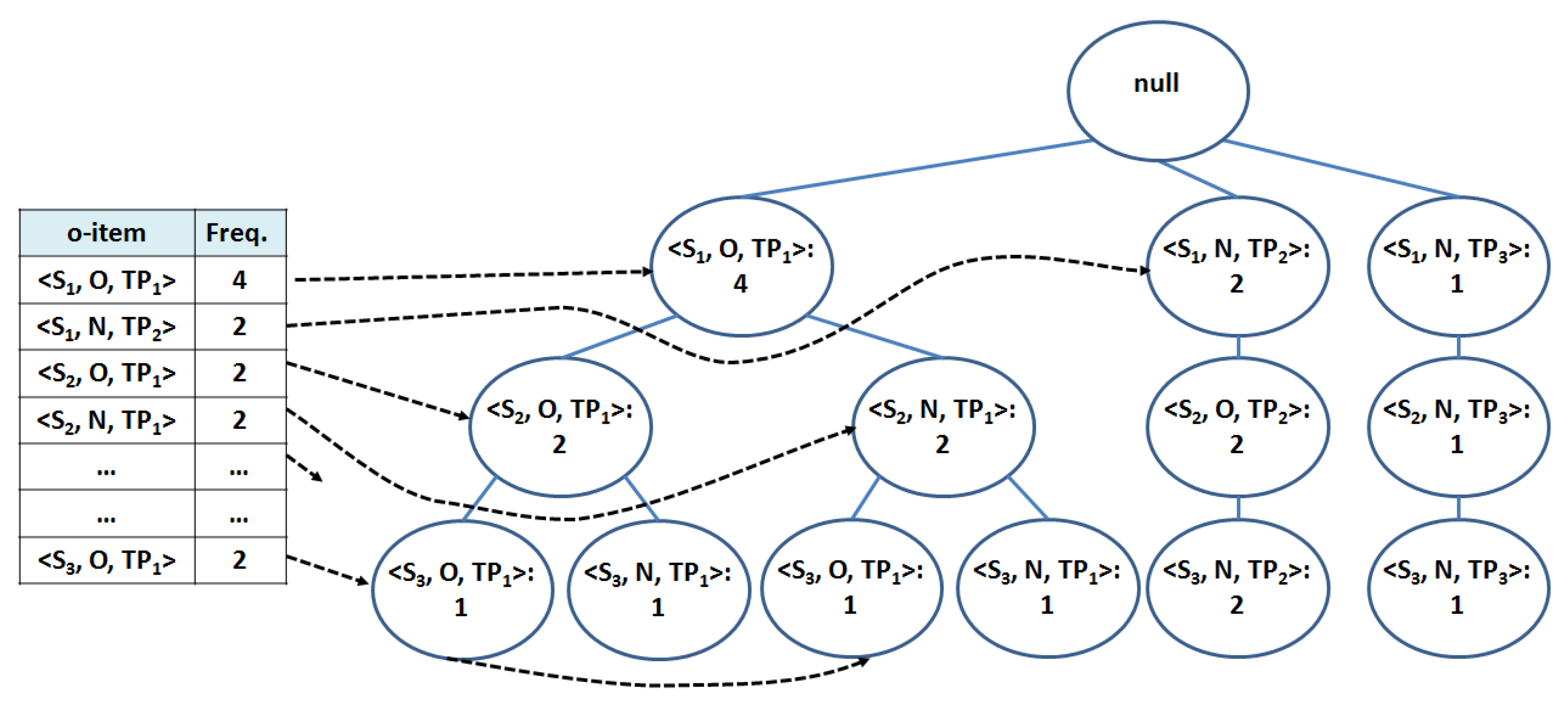
In our context, each node of the tree contains an o-item together with the frequency of the o-item in the path. A transaction in is stored in the FP-tree as a path connecting o-items corresponding to the same time period. Figure 2 reports the FP-tree that represents the transactional dataset in Table 2. For the sake of compactness and readability Overloaded and Normal conditions in o-items are denoted as O and N, respectively. The key advantage of scanning the FP-tree index instead of the original dataset in the o-itemset mining process is that in the FP-tree multiple dataset transactions containing the same o-items are stored in the same path. For example, the FP-tree path [, , ] represents transaction with TID equal to TID, but subpath [, ] represents a common part in transactions with TIDs equal to TID and TID.
The FP-tree is built as follows (Algorithm 1, line 1). For each o-item in , its frequency is computed and stored in a data structure called Header Table. O-items are ordered in the Header Table by decreasing value of their frequency, and they are linked to the FP-tree nodes including them. For the sake of compactness, in Figure 2 only a portion of the whole Header Table is shown. Transactions in are then considered one at time. First, the o-items in the transaction are ordered according to the o-item order in the Header Table; then, the ordered transaction is inserted in the FP-tree using the same approach described in [29].
Phase 2 entails generating all the critical and normal o-itemsets including only nearby stations by recursively visiting the FP-tree (Algorithm 1, line 2). The O-ITEMSETMining algorithm relies on the recursive FP-tree visit adopted by FP-Growth. However, in our proposed approach, the anti-monotonicity property of the spatial constraint (see Section 3.2.1) is exploited to reduce the number of generated combinations. The O-ITEMSETMining algorithm considers one at a time the o-items in the Header Table and generates the o-itemsets including the targeted o-item and a combination of the other o-items in the dataset. For instance, consider the FP-tree in Figure 2. First the o-item = is selected to generate the o-itemsets including it (Algorithm 2, line 3). At this first step the o-itemset I = {} with frequency equal to 2 is extracted.
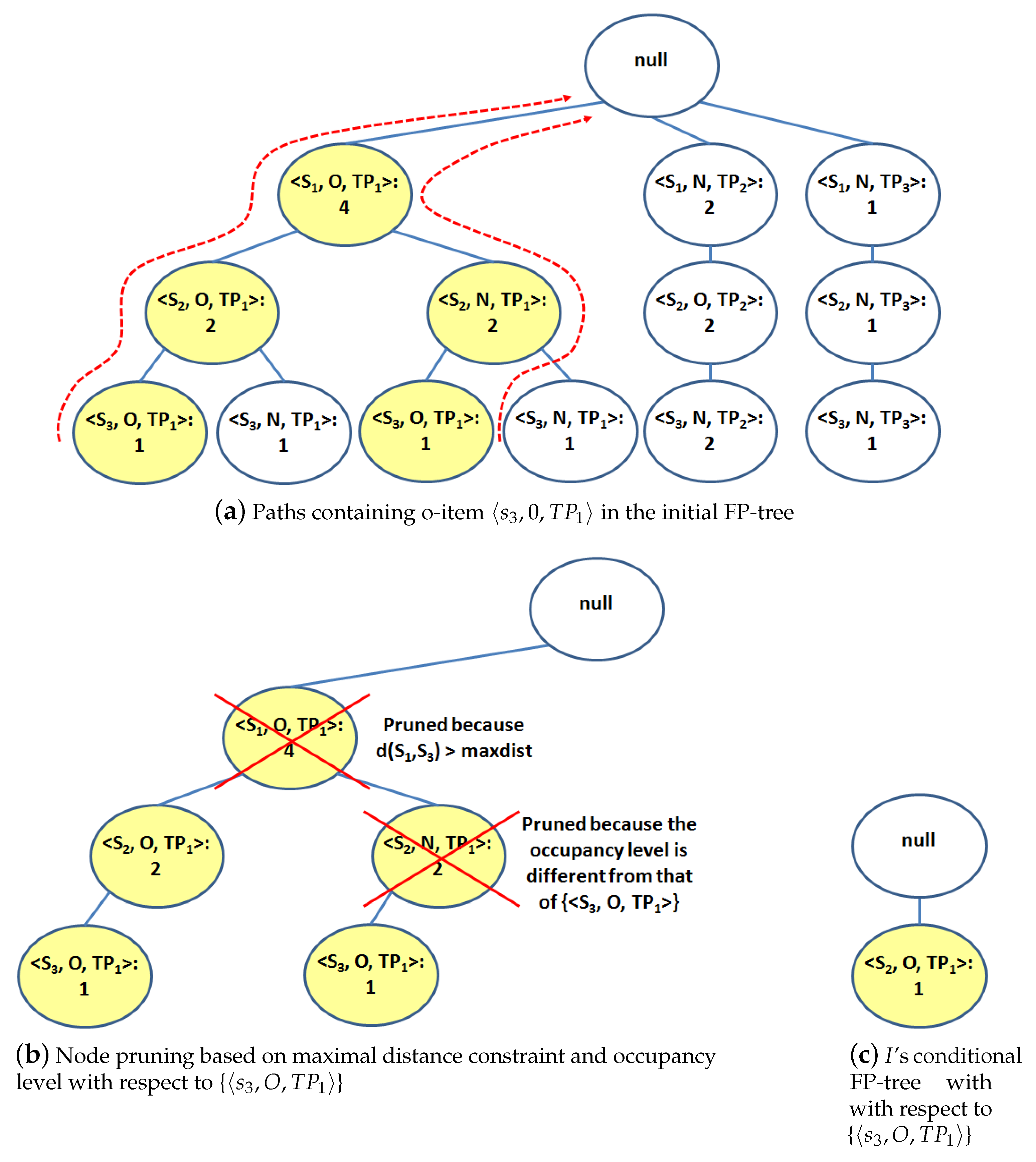
To generate further extensions of the current o-itemset I, the dataset transactions including all o-items in I should be analyzed (Algorithm 2, line 4). These transactions are represented in the FP-tree paths containing all o-items in I. For instance, when I = {}, two FP-tree paths, highlighted in Figure 3a, are selected. These paths represent transactions with TIDs TID and TID. To avoid the generation of useless new o-itemsets, nodes from each selected path are filtered as follows (Algorithm 2, line 5). (i) To guarantee the compliance with the spatial constraint, nodes containing o-items that do not satisfy the maximal distance constraint with o-items in I are discarded. (ii) To guarantee that the o-itemsets are homogeneous in the occupancy level (i.e., all o-items have level Normal or Overloaded), nodes with an occupancy level different from the o-items in I are pruned.
In the example in Figure 3b, two nodes are pruned from the selected paths. (i) We supposed that stations and do not verify the spatial constraint, i.e., > while < . Since the mined o-itemsets cannot contain both stations and , the node with o-item is pruned from the selected paths; (ii) Node with o-item is pruned because its occupancy level is different from the occupancy level in I = {}.
When the pruning phase is concluded, a conditional FP-tree, including only the selected paths is created (using the same approach used in Algorithm 1, line 1) and the O-ITEMSETMining algorithm is recursively invoked on it (Algorithm 2, line 8). This new invocation iterates over the conditional FP-tree with the aim of extending the o-itemset I with the o-items in the conditional FP-tree. A stop condition for the recursive invocation is reached when the conditional FP-tree is empty. In this case, the algorithm backtracks to the previous invocation of the O-ITEMSETMining function; then, it restarts the mining process from there by considering a different o-item in the local FP-tree.
In our running example, the conditional FP-tree associated with the second algorithm invocation contains only o-item . Thus, the o-itemset {, } with frequency equal to 1 is generated. At this point, a stop condition for the recursive invocation has been reached since the conditional FP-tree with respect to the o-itemset {, } is empty. The algorithm backtracks to FP-tree represented in Figure 2 to target the extraction of the o-itemsets including the o-item which precedes item in the Header Table.
Phase 3 aims at generating OMPs by properly combining the critical and normal o-itemsets mined at Phase 2 and stored in sets and , respectively (Algorithm 1, lines 3 and 4).
For each critical o-itemset , an OMP P is generated with criticality and intermittence value computed according to Equations (1) and (2), respectively. For instance, the critical o-itemset {, } with frequency equal to 1 and the normal o-itemset {, } with frequency equal to 1 are mined during Phase 2 from the running example dataset in Table 2. Those two o-itemsets are related to time period , which is associated with four transactions in the running example dataset. Given those two o-itemsets and the number of transactions associated with , the OMP-Miner algorithm extracts the OMP {, } associated with with criticality equal to 1 and intermittence equal to 2.
To efficiently compute the pattern intermittence value, the normal o-itemsets and their corresponding frequency values are stored in a hash map data structure. Given a critical o-itemset , the frequency of the corresponding normal o-itemset including the same stations is returned by the hash map given the key (Algorithm 1, line 7).
| Algorithm 2 O-ITEMSETMining(, maxdist, ) |
| Require:, an FP-tree |
| Require:maxdist: maximum distance between two stations in the same o-itemset |
| Require:, the set of o-items with respect to which FPTree has been generated |
| Ensure:, the set of o-itemsets extending |
| 1: |
| 2: for all o-item = in the header table of do |
| 3: {Generate a new o-itemset I by joining o-itemset and o-item } |
| 4: |
| STATE selectConditionalPaths(, I) {Select I’s conditional paths} |
| 5: applyConstraints(, I) {Prune o-items = such that |
| distance(, ) > maxdist or } |
| 6: createFP-tree(, I) {Build I’s conditional FP-tree} |
| 7: if then |
| 8: O-ITEMSETMining(, maxdist, I) {Recursive mining} |
| 9: end if |
| 10: end for |
| 11: return |
Complexity Analysis
Phases 1 and 2 of OMP-Miner are based on an FP-growth-like mining algorithm. Similar to FP-growth [29], its complexity is linear with respect to the number of mined o-itemsets, which is combinatorial with the number of items, i.e., in the worse case. However, enforcing the spatial constraint allows us to significantly reduce the number of generated itemsets (see Algorithm 2). Finally, the extracted o-itemsets are combined to mine OMPs and compute their quality measures. In addition, this final phase is linear with respect to the number of mined o-itemsets.
3.3. Knowledge Exploration
The OMPs extracted with the OMP-Miner algorithm can be explored by system managers to gain insight into system usage. This explorative analysis allows domain experts to focus their attention on a limited number of stations on given areas and in specific time periods. Based on the mined knowledge, domain experts may recommend targeted maintenance actions with the aims of reducing disruption to end users. To effectively explore the mining result, a list of recommendations is given below.
Exploration of intermittent situations. To detect significant intermittent situations, OMPs should be ranked by decreasing intermittence value. To ease the exploration process, the OMPs with very low intermittence value can be discarded. OMPs with maximal intermittence value indicate groups of stations that are frequently fully occupied in an alternate fashion. These OMPs represent station occupancy level conditions that could result in a limited disservice to the end user. If the stations in the OMP are located in the same area, then an alternative arrival station can be recommended to users who reach an occupied station. The severity of the possible disservices for end users can vary based on the criticality value of the OMP. When the pattern criticality level increases, the stations indicated by the OMP are more frequently fully occupied at the same time; thus, end users are unlikely to find a free dock at nearby stations.
To avoid disservices, system managers can suggest an alternative nearby station with free docks for parking; in case of OMPs with high intermittence but low criticality values, bicycles may be repositioned in nearby stations because they are rarely fully occupied at the same time.
Exploration of critical situations. In order to detect significant critical situations which could lead to serious disservice for end users, OMPs should be ranked by decreasing criticality value. To ease the exploration process, the OMPs with very low criticality value can be discarded. OMPs with maximal criticality value indicate groups of nearby stations that are frequently fully occupied at the same time. Thus, end users are unlikely to find free docks for their bikes in this area.
Since nearby stations are all fully occupied, maintenance actions such as bicycle repositioning should be carried out considering stations that are further away or located in other areas of the city. Therefore, to address these issues, maintenance actions could be much more expensive or even inapplicable. Alternative actions could be considered such as planning station resizing or system enlargement.
Exploration of the spatio-temporal distribution of intermittent and critical situations. To support management of the bicycle sharing system, the mined OMPs can be visualized on a map of the city area. Since each station in the OMP is characterized by a geographical position, OMPs can be represented as restricted city areas including the corresponding stations. This representation is intuitive and effective for highlighting the areas which could lead to disservices for end users. OMP representations can be differentiated based on the type of imbalance in station occupancy (i.e., critical, intermittent) and the degree of severity of the discovered pattern. Domain experts can also analyze intermittent and critical situations for different values of time periods to identify the time frames associated with more serious disruptions. For example, they can consider 1-h time slot as time period to analyze the number and significance of intermittent and critical situations for each hour in a day. Alternatively, they can adopt a courser time granularity, as a larger time slot size (e.g., morning, afternoon, evening, night), to gather a more high-level view of the dock overload conditions in the bicycle sharing system.
Domain experts are recommended to adhere to the following guideline in order to properly set up the OMP-Miner algorithm. The spatial constraints maxdist should be set according to the geographical distribution of the stations in the city area. For example, stations located at a walking distance can be considered as near while stations located in different districts can be classified as distant. To ensure that the extracted OMPs include only close stations, the user should set maxdist as the largest distance between a pair of nearby stations.
Some examples OMPs representing significant intermittent and critical situations in real data collections, and the analysis of their spatio-temporal distribution, are reported in Section 4.
4. Experimental Results
The efficiency and usability of the BELL system on real data acquired from bicycle sharing systems were validated in two important cities: Barcelona, the capital city of the autonomous community of Catalonia and Spain’s second most populated city and New York, the most populated city in the United States of America.
The experimental evaluation addresses the following aspects. Some examples of interesting OMPs representing significant intermittent and critical situations, extracted from the analyzed data collections, are presented in Section 4.2. Section 4.3 evaluates the impact of the system configuration parameters on the number of mined OMPs and on their corresponding intermittence and criticality values, while Section 4.4 reports performance evaluation in terms of execution time for the OMP-Miner algorithm. The main characteristics of the analyzed datasets are summarized in Section 4.1.
The OMP-Miner algorithm was implemented by using the C language. The experiments were performed on a 2.67 GHz six-core Intel(R) Xeon(R) X5650 machine (Turin, Italy) with 32 Gb of main memory running Ubuntu 18.04 server with the 3.5.0-23-generic kernel.
4.1. Reference Use Case Datasets
This section briefly presents the main characteristics of the two bike sharing systems considered as reference use case in this study and describes data that we have considered on the system usage.
The Bicing system in Barcelona. Bicing is the bicycle sharing system in Barcelona which consists of 377 stations distributed all over the city area. Stations have a fixed number of parkings, which vary from 15 to 39. A description of the service is given in [13]. To perform our analyses, the collection of measurements described in [13] have been taken into account. The acquired data (from a single operator) include 30 million records from the Bicing stations over a period of approximately a semester of service (i.e., between 15 May and 30 November 2008). Occupancy values were acquired every 5 min.
The Citi Bike system in New York.Citi Bike is the bicycle sharing system in New York which features thousands of bikes at 528 stations across New York and Jersey City. Bicycles are available 24/7, 365 days a year. More information about the system is given in [2]. To perform our analyzes, an ad hoc Web crawler was developed which downloaded and parsed the JSON data from the Citi Bike system feed to retrieve the historical occupancy data. Occupancy values were acquired every 5 min over a time period of approximately 13 months (i.e., between 23 October 2014 and 17 November 2015).
Characteristics of the collected data on the system usage. In both bicycle sharing systems, each station is characterized by the information on its name and geographic coordinates (latitude and longitude). Historical data on station occupancy can be collected by submitting periodical requests to the stations in the system and storing the corresponding responses. Specifically, for each station, we acquired the information on the number of free and occupied slots in different time instants within a given time window.
4.2. OMP Characterization
In what follows, some OMPs are discussed as representative examples of the insights mined through our framework. Specifically, some top ranked OMPs with maximal intermittence and criticality values are discussed as reference cases. These OMPs represent dock overload conditions that could yield to disservices for end users in the usage of the bicycle sharing system.
OMPs were extracted from the Bicing and Citi Bike datasets using a standard system configuration with maxdist = 0.5 km, full-th = 3, and time period equal to time slot size of 1 h.This configuration pinpoints a time-space granularity suitable to provide useful information to end users and system managers. For example, we set maxdist = 0.5 km because bikers are (usually) more willing to move to physically closer stations if the expected destination is fully occupied. We set the time period equal to time slot size = 1 h to determine more precisely sets of nearby stations that could lead to service disruption. Parameter full-th has been set to 3 to represent situations when the station is (almost) full. The impact of the system parameters on the characteristics of the extracted OMPs is discussed in Section 4.3.
Example OMPs with maximal intermittence. The OMP-Miner algorithm generates as output a set of OMPs with various intermittence values. The intermittence measure of an OMP is computed to measure the presence of a dock overload condition from the occupancy levels of the corresponding stations (see Algorithm 1, line 7). The higher the intermittence value, the more severe the imbalance condition. Hence, OMPs with highest intermittence values should be considered first in the result exploration.
Table 3 and Table 4 report some examples of top ranked OMPs with maximal intermittence value extracted from the Bicing and Citi Bike datasets, respectively. In both tables, OMPs are sorted by decreasing intermittence value. The example OMPs from the Bicing dataset (Table 3) are characterized as follows.
OMPs with identifiers (IDs) 5–7 represent dock overload conditions that could yield a limited disservice for end users. Each of these OMPs represents a group of stations that the end user is likely to find fully occupied in alternate fashion (in about 62–63% of the recorded timestamps according to the intermittence value). However, the low criticality values of these OMPs point out that the stations in each OMP are rarely fully occupied at the same time (in about 0.13–1.56% of the cases). It follows that, in case the user is unable to park in one station, she/he can move to another nearby station where free parking docks will be available with a high probability. For example, OMP with ID 5 indicates that the usage levels of stations Carrer de Bonavista and Pl. del Poble Romaní are critical in an alternate fashion from 7:00 a.m. to 8:00 a.m. in 63% of the cases, but they are fully occupied at the same time only in 1.56% of the cases.
On the other hand, OMPs with IDs 1–2 represent dock overload conditions that could result in a more serious disservice for end users. Each of these OMPs models a group of stations having both intermittence and criticality values higher than OMPs with IDs 5–7. For each OMP, at least one station has a high probability of being occupied (intermittence value higher than 71%), and all stations have a non-negligible probability of being fully occupied at the same time (criticality about 8%). Therefore, in case the user cannot park in one station, she/he might not find a free dock at a nearby station approximately 8% of the time. As an example, OMP with ID 1 shows that, from 4:00 a.m. to 5:00 a.m., stations Vilamara davant, Mallorca and Calabria have a critical usage level in an alternate fashion in 73.84% of the recorded timestamps, and they are simultaneously fully occupied in 8.29% of the cases.
OMPs with IDs 3-4 represent an intermediate condition between the two above. These OMPs have intermittence and criticality values higher than OMPs with IDs 5–7 (intermittence 70–71% instead of 63% and criticality 1.86–4% instead of 0.13–1.56%), but lower than OMPs with IDs 1–2 (intermittence 70–71% instead of 73% and criticality 1.86–4% instead of 8%).
Based on the mined knowledge, domain experts may recommend an alternative nearby station for parking and/or targeted maintenance actions. For instance, they may decide to relocate bicycles at the beginning of the time slot, moving them from stations with critical levels to non-critical stations.
Compared to the OMPs extracted from the Bicing dataset, the top ranked OMPs mined from the Citi Bike dataset have very high intermittence values (between 90% and 100%) and criticality equal to 0% (Table 4). For example, OMP with ID 2 consists of four nearby stations ({W 33 St & 8 Ave, W 29 St & 9 Ave, W 31 St & 8 Ave, Penn Station Valet}) with 100% intermittence and 0% criticality from 8:00 p.m. to 9:00 p.m. These stations are close to Madison Square Garden Stadium and Pennsylvania Station, which are big subway and train hubs. These OMPs indicate conditions which could lead to a limited disservice for the end users. On the one hand, since the OMP intermittence value is very high, at least one of the stations in the OMP is likely to be fully occupied, while, on the other hand, since the criticality value is 0%, at least one station has a free dock in all the recorded timestamps. Consequently, the user will probably find a free dock among nearby stations.
Example OMPs with maximal criticality. The OMP-Miner algorithm computes the criticality of each of the mined OMPs (see Algorithm 1, line 4). The criticality measure indicates the unavailability of most of the docks in a set of stations. The higher the criticality, the more critical the situation of imbalance that need to be faced.
Example OMPs with maximal criticality. The OMP-Miner algorithm computes the criticality of each of the mined OMPs (see Algorithm 1, line 4). The criticality measure indicates the unavailability of most of the docks in a set of stations. The higher the criticality, the more critical the situation of imbalance that need to be faced.
Table 5 and Table 6 report the top ranked OMPs with maximal criticality value mined from the Bicing and the Citi Bike dataset, respectively. OMPs in Table 5 and Table 6 represent potentially severe disservices for the end users of the system because they identify groups of nearby stations whose levels of usage are frequently all critical at the same time.
For example, for the Bicing in Table 5, OMP with ID 1 indicates that from 10:00 a.m. to 11:00 a.m. stations Marquas de l’Argentera and Avinguda del Marques Argentera (approximated distance 300 m) both have critical usage levels in approximately 38% of the recorded timestamps. Thus, one third of the time the parking is unavailable in this time slot in the mentioned areas. If the problem persists, users working or living in the neighborhood are strongly discouraged from using the service. Since nearby stations are all fully occupied, maintenance actions such as bicycle repositioning should be carried out considering stations that are further away or located in other areas of the city. Therefore, in order to address these issues, maintenance actions could be much more expensive or even not feasible.
Results in Table 6 report even more critical situations for some groups of stations in the Citi Bike dataset. For instance, OMP with ID 1 representing the nearby stations E 85 St & 3 Ave and E 84 St & 1 Ave has a criticality equal to 51%. Hence, in half of the cases, both stations are fully occupied.
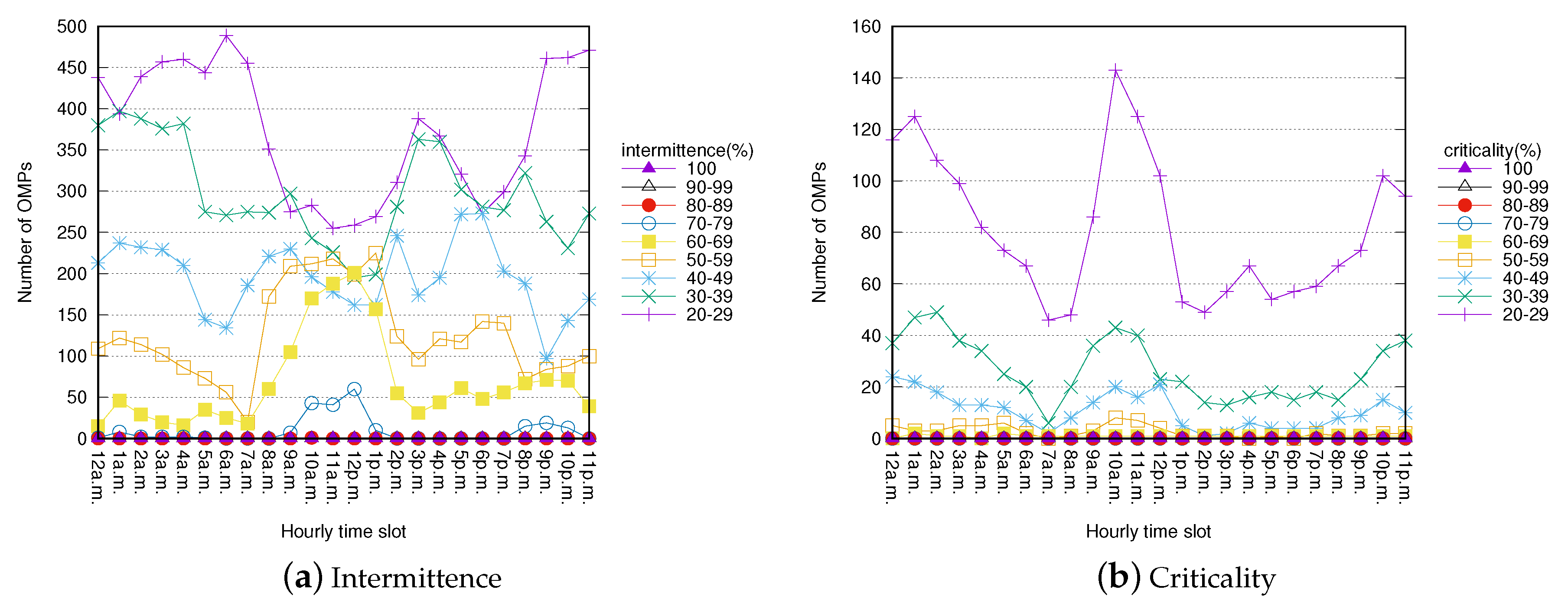
Hourly distribution of intermittent/critical OMPs. The OMP-Miner algorithm allows us to extract OMPs and store their criticality/intermittence values in different time slots (see Algorithm 1, line 5). Analyzing the quality measures in different time slots allows domain experts to detect time-constrained imbalance situations (e.g., situations arising in specific hourly time slots).
Figure 4 and Figure 5 show the hourly distribution of the number of OMPs and their corresponding levels of intermittence and criticality. The two figures report, for each hourly time slot, the total number of mined OMPs characterized by different ranges of intermittence and criticality values. In order to identify OMPs that could lead to a disservice for end users, OMPs with an intermittence/criticality value greater than or equal to 20% have been taken into consideration.
In the Bicing dataset (Figure 4), a significant number of OMPs with intermittence/criticality values greater than or equal to 20% occurs in all hourly time slots. However, OMPs with higher values of intermittence/criticality mainly occur between 1:00 a.m. and 2:00 a.m., between 7:00 a.m. and 1:00 p.m., and between 4:00 p.m and 11:00 p.m.
OMPs mined from the City Bike dataset (Figure 5) show a similar hourly distribution to OMPs from the Bicing dataset. However, a lower number of OMPs with high intermittence/criticality values comes from the City Bike dataset, probably because the stations in New York are more widespread than those in Barcelona.
Domain experts can thus gather useful insights on the usage of the bicycle sharing system. On the one hand, they can identify daily time periods in which service disruptions may occur, and, on the other hand, they can also identify the set of nearby stations which are involved in these disservices.
Geographical distribution of significant intermittent and critical OMPs. Each OMP represents a group of geo-referenced stations. To support the management of the bicycle sharing system, maps can be used to highlight the city areas associated with OMPs (i.e., groups of stations) with high intermittence and criticality values. Notice that OMPs can be easily visualized on a map because they represent groups of nearby stations. The extraction and visualization of OMPs including distant stations is prevented by enforcing the spatial constraint in the OMP-Miner algorithm (see Algorithm 2, line 5).
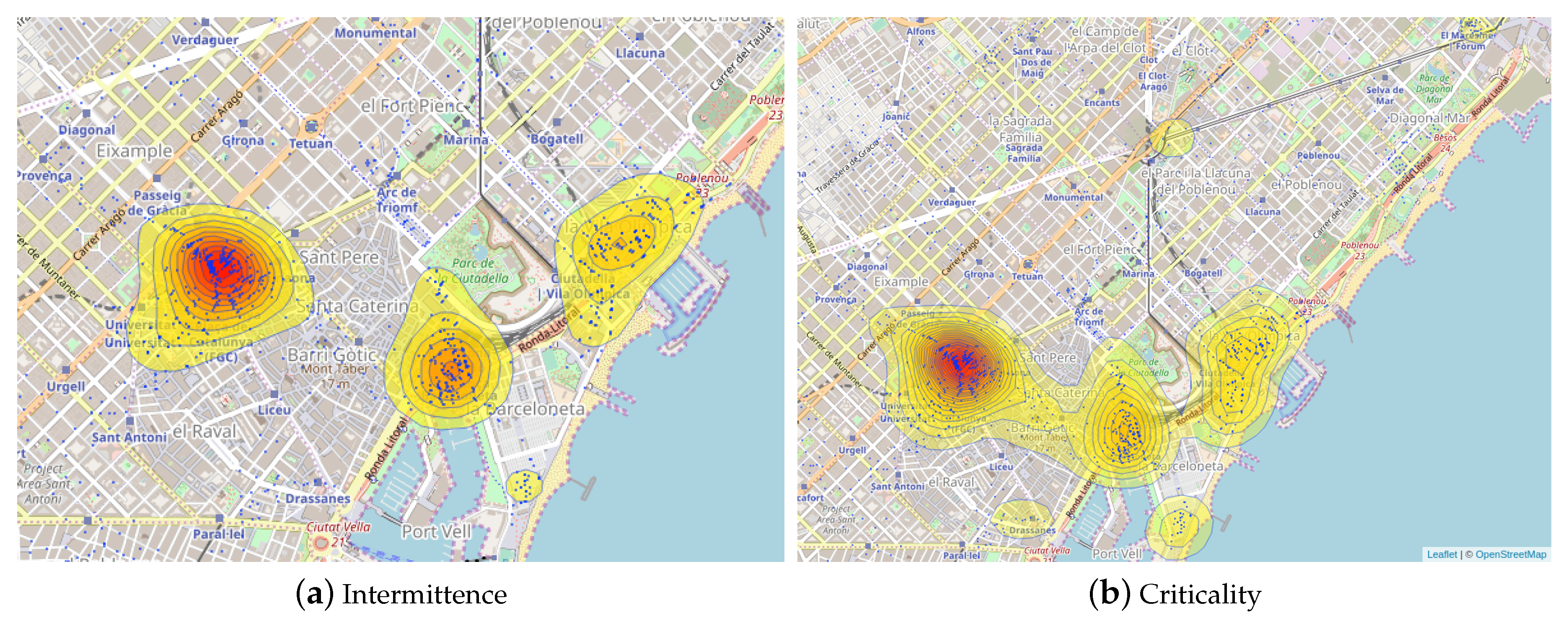
For example, Figure 6a,b show two heat maps (The heat maps have been generated by using the service provided by Babicki et al. [31].) of the areas of Barcelona identified by the OMPs in hourly time slot (between 11:00 a.m. and 12:00 a.m.). OMPs in this time slot represent significant intermittent and critical situations according to the results in Figure 4. In Figure 6a,b, the color intensity of areas increases with the density of occurrence of OMPs and their intermittence and criticality values, respectively. The higher the color intensity, the more severe the disservice to end users.
Figure 6a shows that intermittent situations are mainly localized in the city center in four distinct areas. The area with the highest intensity is centered in Placa Catalunya, while the other two large areas are centered in History Museum of Catalonia and La Vila Olimpica del Poblenou and a small area is in Pla de Miquel Tarradell.
Instead, based on Figure 6b, critical situations are more spread over the geographical areas. The larger area in Figure 6b covers all the three main areas in Figure 6a. Moreover, three additional areas show up, two of them located on the top of the map (in the Torre Glories and El Maresme Forum areas) and one on the bottom (Drassanes area).
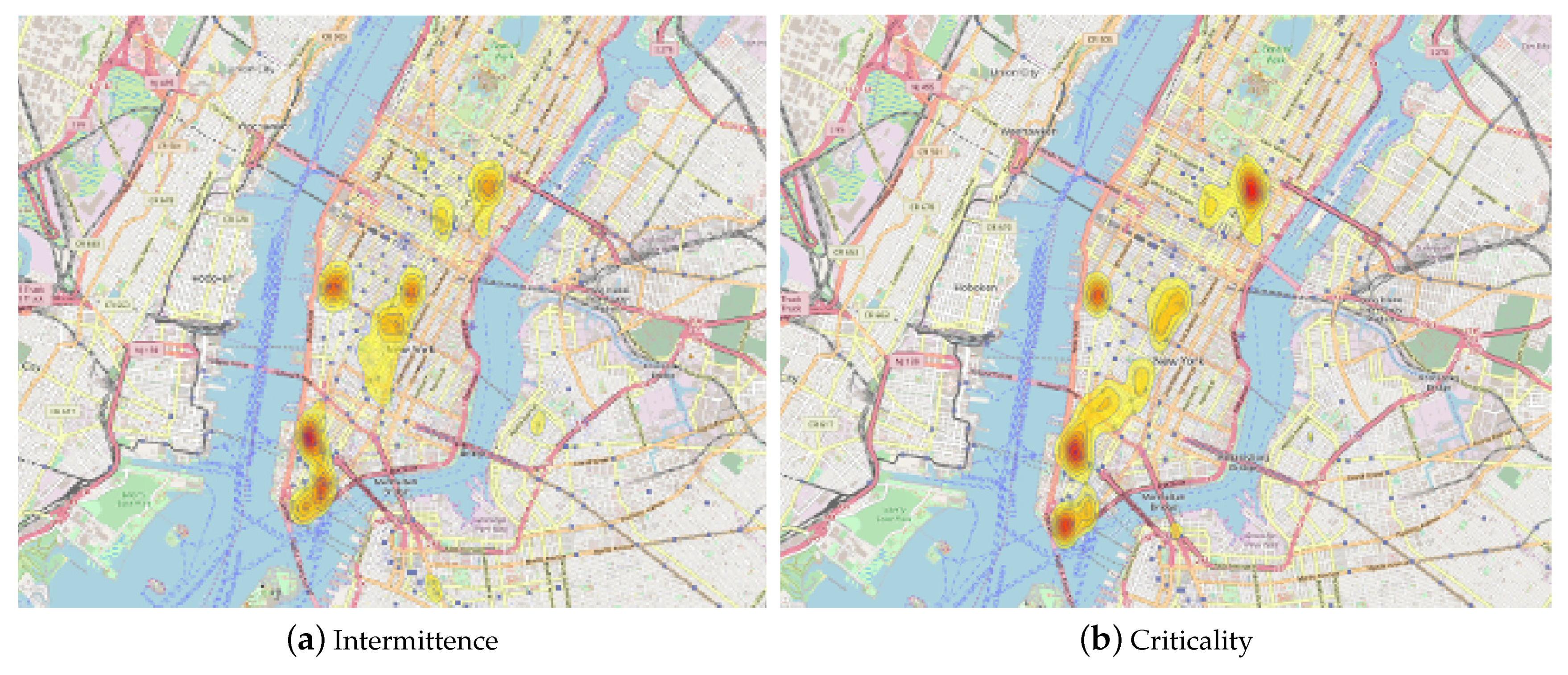
We also exploited heat maps to analyze the geographical distribution of OMPs mined in hourly time slot (between 11:00 a.m. and 12:00 a.m.) in New York (see Figure 7a,b). Compared to Barcelona, more areas in New York are characterized by OMPs with high intermittence and criticality values. The areas with the highest intensity for intermittence situations are mainly located in the World Trade Center (on the bottom of the map), while the highest intensity for critical situations is located both in the areas of the World Trade Center and of the Museum Of Modern Art (on the top of the map).
4.3. Parameter analysis
The main parameters of the OMP-Miner algorithm are as follows: (i) The threshold used to discriminate station occupancy levels into Normal and Overloaded, i.e., the occupancy threshold full-th; (ii) the threshold used to decide whether two stations are located nearby or not, i.e., the maximum distance threshold maxdist; and (iii) the time granularity used to analyze the evolution of imbalance situations over time, i.e., time slot size.
We analyzed the impact of parameters full-th, maxdist, and time slot size on (i) the cardinality of the mined OMPs (i.e., the number of OMPs per time slot), (ii) the distribution of the intermittence values of the mined OMPs, and (iii) the distribution of the criticality values of the mined OMPs. Moreover, we also analyzed the impact of the day category on the hourly distribution of the intermittence and criticality values for the mined OMPs.
In the experimental evaluation, we varied one parameter at a time, and we set the standard configuration for the remaining parameters. The standard configuration was introduced in Section 4.2 as maxdist = 0.5 km, full-th = 3, time slot size = 1 h.
For the sake of brevity, we will hereafter report the results achieved on the Bicing dataset (Barcelona) considered as a reference example study. Similar results have been obtained from the Citi Bike dataset.
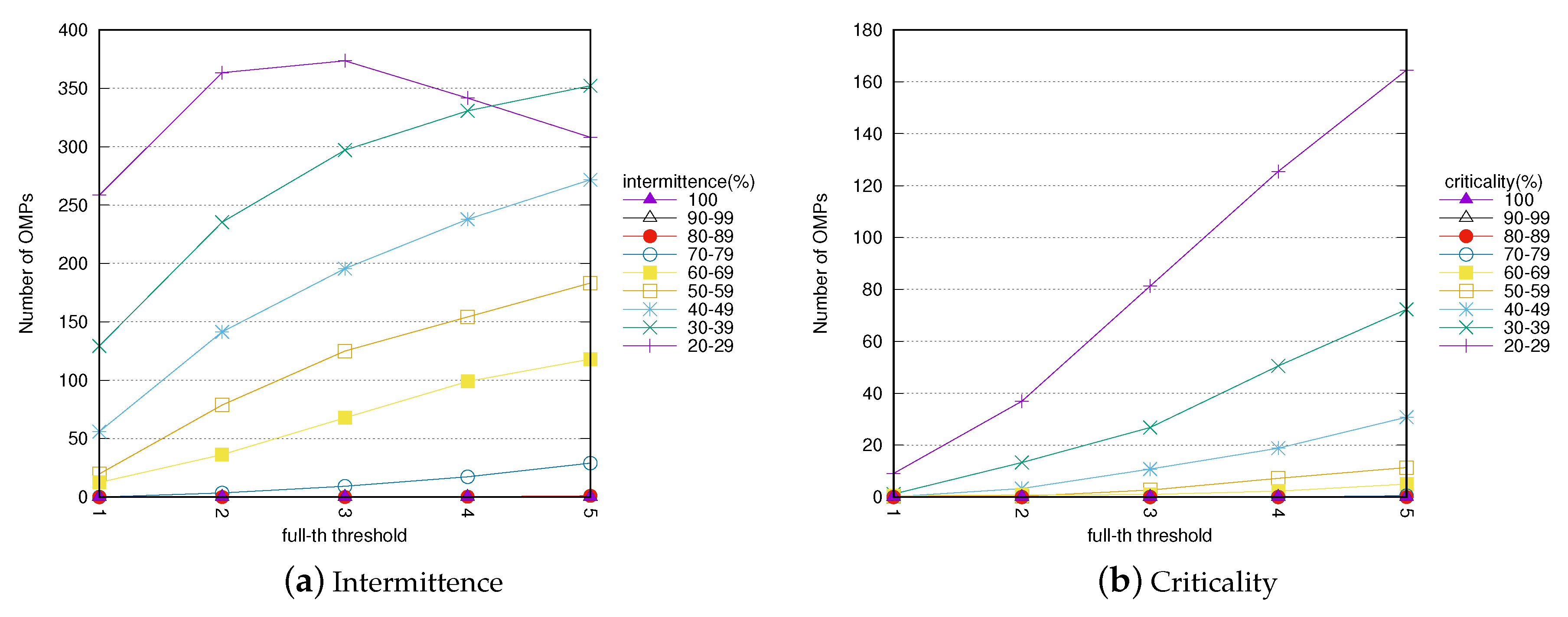
Occupancy threshold (full-th).Figure 8a,b show the impact of the full-th parameter on the mined OMPs. The two figures report the total number of mined OMPs for each range of intermittence and criticality value when increasing full-th.
A station is in an overloaded condition when less than full-th free docks are available. Therefore, the higher occupancy threshold value we set, the more OMPs with high intermittence/criticality value could be extracted. The results reported in Figure 8a,b show this trend. The number of OMPs for each intermittence and criticality range increases almost linearly when increasing the full-th value. This increase is higher for the intermittence index.
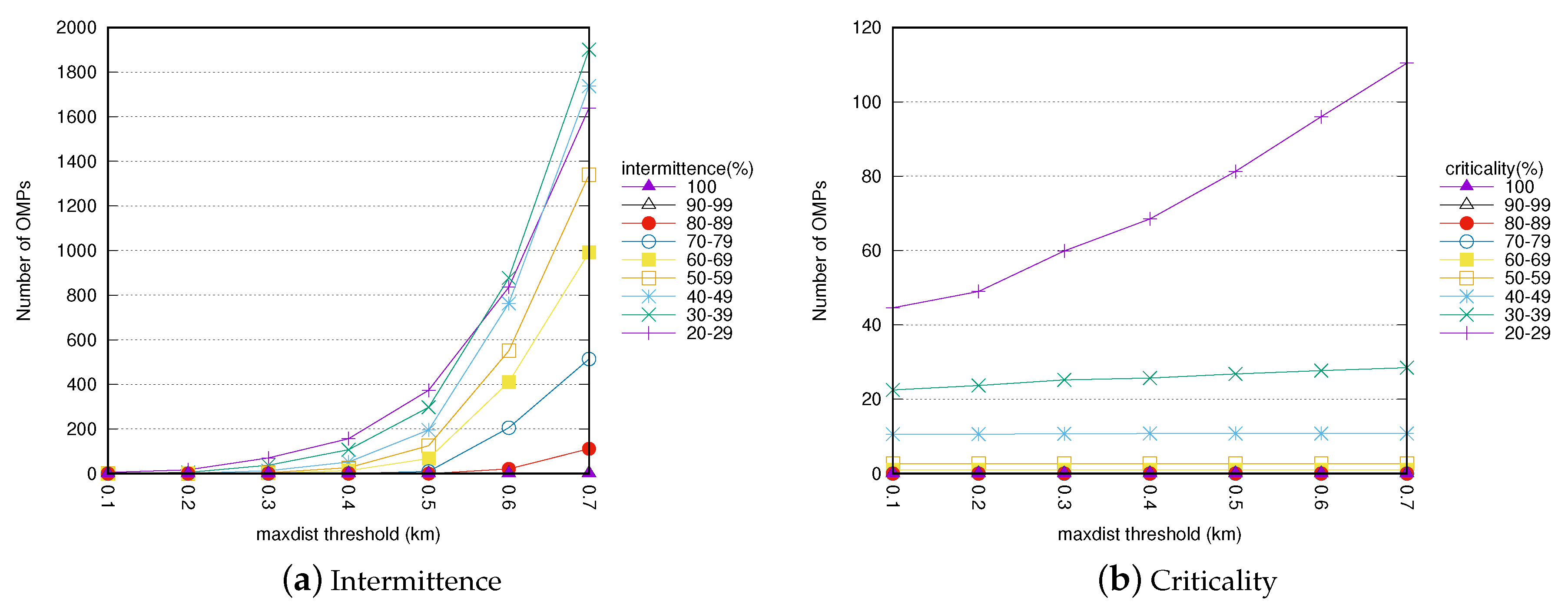
Maximum distance threshold (maxdist).Figure 9a,b show the impact of the maxdist parameter on the number of mined OMPs. The two figures report the total number of mined OMPs for each range of intermittence and criticality value when increasing maxdist.
When the maxdist value is increased, the number of nearby stations also increases. Consequently, the number of mined OMPs increases because larger patterns including more stations are also generated. Results show that when increasing maxdist the number of OMPs increases almost exponentially for each intermittence range and almost linearly for each criticality range.
However, the number of OMPs that are worth considering for manual inspection (i.e., those with high intermittence/criticality values) remains roughly stable even while enforcing maxdist values higher than 0.5 km. Setting maxdist values higher or equal to 0.6 km is less interesting in our context of analysis because the end users are willing to move to physically closer stations if the expected destination is fully occupied.
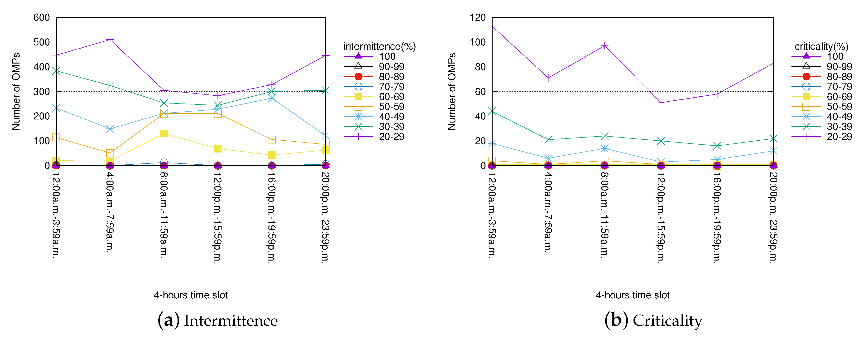
Time slot size. The distribution of the number of extracted OMPs for each intermittence and criticality range when varying the time slot size were also analyzed. Experiments were performed for time slots ranging from two to eight hours; as a representative example, Figure 10 reports the results achieved on the Bicing dataset with the 4-h time slot.
Considering a courser time granularity to analyze collected data as, for example, a larger time slot size, can provide a high-level view of the station overload conditions in the bicycle sharing system. This view can be useful for end users but expecially for system managers to identify the time frames when usage conditions are critical. For instance, results in Figure 10a point out that the number of OMPs with high intermittence value (between 50–59%) is significantly higher between 8.00 a.m. and 12:00 p.m.
Domain-experts can then focus on each selected time frame to locally analyze collected data with a finer time granularity (i.e., a time slot with lower size). This latter analysis can provide more detailed information on dock overload conditions on each selected time frame.
In some cases, using time slots with a larger size could smooth local intermittence and criticality peaks of potential interest. For instance, few OMPs with intermittence in the range 70–79% are mined with a 4-h time slot (see Figure 10a). Instead, when considering 1-h time slots, around 50 patterns with intermittence between 70–79% are generated in the 10:00 a.m., 11:00 a.m., 12:00 p.m. time slots (see Figure 4a).
Day category. Experiments have been performed to analyze the impact of the day category on the hourly distribution of intermittence and criticality. We compared the OMPs extracted by considering the station occupacy log data related to workdays with respect to those mined by considering the weekends. Results are shown in Figure 11a–d.
Extracted OMPs show a significantly different trend in weekdays and weekends. More OMPs with higher criticality and intermittence values are mined in weekdays. These OMPs are mainly located in the time period from 7:00 a.m. to 2:00 p.m. In weekends, OMPs with high intermittence and criticality values (about 70–79%) are mainly related to the period from 12:00 a.m. and 1:00 a.m. and from 7:00 p.m. to 11:00 p.m. Moreover, OMPs with high intermittence values are also mined for the 2:00 p.m. time slot.
These results highlight different usages of the bike sharing system of Barcelona during the days of the week. They support the need for different actions (such as bike rebalancing actions) depending on the type of day of the week we are considering. For example, bike rebalancing actions may be more relevant in weekdays than in weekends, and they must be scheduled in different time periods based on the day category.
4.4. Algorithm Performance
We analyzed the performance of the OMP-Miner algorithm in terms of execution time. OMP-Miner requires time both for (critical and normal) o-itemset extraction and for the consequent generation of OMPs on top of the mined o-itemsets. The o-itemsets extraction is the most computationally expensive step. With the default parameter setting, the extraction time of o-itemsets is approximately 454 s for Bicing (Barcelona) and 825 s for Citi Bike (New York), while the time for OMP generation is a few milliseconds in both cases.
We also analyzed how the system parameters impact on the execution time. Specifically, we focused our analysis on the maximum distance threshold maxdist, which can impact significantly on the number of mined OMPs, and thus on the execution time. Experiments were run by varying the maxdist value while the standard configuration was adopted for the other parameters. The execution time, similarly to the number of mined OMPs, increases more than linearly with respect to the maximum distance threshold value. The time ranges from 3 min when maxdist = 0.1 km up to 42 min when maxdist = 0.6 km. The execution time increases to more than one hour when values of maxdist greater than 0.6 km are used, i.e., when maxdist is set to values that are considered not interesting in our application domain. Most of the execution time is spent on o-itemset generation, while even in the worst case the OMP generation requires a few seconds.
5. Discussion
The BELL methodology analyzes historical occupancy data acquired from bicycle sharing systems with the aim of identifying situations of imbalance in dock occupancy levels of bike stations. The proposed methodology relies on an itemset-based approach, which extracts recurrent patterns from historical data and provides domain experts with a set of interpretable patterns to explore. The extracted OMPs describe the context (i.e., city area and time slot) in which a set of stations is in a critical/intermittent dock overload condition. The discovered patterns represent (i) groups of nearby stations whose slots are almost all occupied at most points of time, and (ii) groups of nearby stations among which at least one of them (but not all of them) has a high level of occupancy at most points of time (possibly in an alternate fashion).
The position of this paper differs to a large extent from previous works in the literature. Specifically, (i) previous works on clustering of the stations based on their usage profiles have been unable to identify intermittent dock overload situations; (ii) studies on forecasting future occupancy levels of the stations have applied supervised techniques, while the methodology presented in this paper relies on an unsupervised technique (i.e., itemset mining); (iii) previous approaches aimed at planning re-balancing actions are complementary to the proposed work because they can be applied to a subset of stations with intermittent dock occupancy levels.
The results achieved by the BELL methodology on real bicycle sharing system data have shown potentially harmful dock overload situations in the stations of bike sharing systems. Specifically, we explored the applicability of the BELL methodology in two real case studies, the Barcelona and New York bicycle sharing systems. Notably, the achieved results show behaviors peculiar to each use case. For example, in New York, the mined OMPs highlight situations of imbalance mainly due to intermittent occupancy levels (i.e., intermittence value = 100%, criticality value = 0%). This implies that, although some areas were characterized by a strongly imbalanced bike distribution among stations in certain time slots, at least one station per area had a non-critical dock occupancy in the analyzed period. Hence, planning re-balancing actions could be sufficient to counteract situations of imbalance. Conversely, in Barcelona, situations of imbalance were usually characterized by a mix of critical and intermittent conditions. Hence, re-balancing actions may not be sufficient and long-term maintenance actions (e.g., station resizing) need to be put in place to counteract the issue.
The takeaways from this study can be summarized as follows:
- The use of data mining tools to analyze bicycle sharing system data has become more and more attractive.
- Unsupervised approaches, like the BELL methodology presented in this study, characterize system usage in the medium and long-term. They identify contexts in which user experience could worsen due to recurrent system inefficiencies.
- System users may take advantage of the data-driven approaches to system monitoring because potentially critical situations can be automatically detected and managed without the need for explicit notification.
- Urban policymakers can exploit the BELL methodology to periodically monitor the dock overload situations detected in specific city areas at different time slots.
- Based on the knowledge extracted by the BELL methodology, policymakers could put in place medium-term actions, such as rebalancing actions triggered by the extraction of OMPs with high intermittence value, and long-term actions, such as station resizing or new station placement triggered by the extraction of OMPs with high criticality value.
- The results in the real case studies demonstrated the quality of the proposed methodology in supporting system managers under various aspects.
As future work, we plan to integrate other data sources to enrich the quality of the generated model. Variables such as the presence of environmental pollution, road network features, vehicular traffic, and the presence of cycling lanes as indicators of favorable/unfavorable conditions for bike sharing system usage will also be taken into consideration. In parallel, we will investigate the portability of the proposed methodology for different mobility services offered in urban contexts. For example, we plan to apply the proposed approach to charging stations of electric cars and to indoor car parks.
6. Conclusions
This study presented a novel exploratory data-driven methodology, named BELL. It identifies situations of dock overload in multiple stations which could lead to either service disruption or low customer satisfaction. To describe in a concise way situations of imbalance in the occupancy levels of spatially correlated stations, it proposes a new type of pattern, called Occupancy Monitoring Pattern. The achieved results demonstrated the effectiveness of BELL in identifying useful knowledge regarding the spatio-temporal distribution of possible service disruptions for end users of bicycle sharing systems. Possible scenarios of usage of the mined patterns, such as supporting maintenance activities and improving user experience, were discussed.
Author Contributions
Conceptualization, L.C., S.C. and P.G.; Funding Acquisition, S.C.; Investigation, P.G. and G.R.; Methodology, L.C., T.C., S.C. and P.G.; Software, G.R.; Supervision, S.C. and E.B.; Writing—Original Draft, L.C. and S.C.; Writing—Review and Editing, L.C., T.C., S.C. and P.G.
Funding
The research leading to these results was partially funded by the Italian Ministry of Research (MIUR) under the smart cities and Communities Grant Agreement n. SCN_00325 (Project s[m2]art).
Conflicts of Interest
The authors declare no conflict of interest.
Appendix A

Table A1.
Notation.
| Symbol | Description |
|---|---|
| Reference time window | |
| Set of points of time in | |
| Station of the bicycle sharing system | |
| occupancy level of station at any timestamp | |
| Set of stations | |
| Occupancy level dataset in relational format | |
| Dataset record corresponding to timestamp | |
| Occupancy level dataset in transactional format | |
| Record identifier | |
| Transaction identifier | |
| P | Occupancy Monitoring Pattern |
| maxdist | Spatial constraint |
References
- Shaheen, S.; Martin, E. Unraveling the modal impacts of Bikesharing. Access Magazine, 2009; 8–15. [Google Scholar]
- Martin, E.; Chan, N.; Cohen, A.; Pogodzinski, M. Public Bike sharing in North America During A Period of Rapid Expansion: Understanding Business Models, Industry Trends and User Impacts; Technical Report; Mineta Transportation Institute: San Jose, CA, USA, 2014. [Google Scholar]
- Susan, S.; Martin, E.; Cohen, A. Bikesharing and Modal Shift Behavior: A Comparative Study of Early Bikesharing Systems in North America. Int. J. Sustain. Transp. 2013, 1, 35–54. [Google Scholar] [CrossRef]
- Natalie, B.; Buck, D.; Chung, P.; Happ, P.; Kushner, N.; Maher, T.; Rawls, B.; Reyes, P.; Steenhoek, M.; Studhalter, C.; Watkins, A.; Buehler, R. Virginia Tech Capital Bikeshare Study; Technical Report; Virginia Tech: Blacksburg, VA, USA, 2012. [Google Scholar]
- Gleason, R.; Miskimins, L. Options for Federal Lands: Bike Sharing, Rentals and Employee Fleets; Technical Report; Western Transportation Institute: Bozeman, MT, USA, 2012. [Google Scholar]
- Wang, S.; Zhang, J.; Liu, L.; Duan, Z.Y. Bike-Sharing-A new public transportation mode: State of the practice and prospects. In Proceedings of the 2010 IEEE International Conference on Emergency Management and Management Sciences (ICEMMS), Beijing, China, 8–10 August 2010; pp. 222–225. [Google Scholar]
- Shaheen, S.; Guzman, S.; Zhang, H. Bikesharing in Europe, the Americas, and Asia: Past, Present, and Future; UC Davis: Institute of Transportation Studies (UCD): Davis, CA, USA, 2010; pp. 8–15. [Google Scholar]
- Zheng, Y.; Capra, L.; Wolfson, O.; Yang, H. Urban Computing: Concepts, Methodologies, and Applications. ACM Trans. Intell. Syst. Technol. 2014, 5, 38:1–38:55. [Google Scholar] [CrossRef]
- Etienne, C.; Latifa, O. Model-Based Count Series Clustering for Bike Sharing System Usage Mining: A Case Study with the Velib System of Paris. ACM Trans. Intell. Syst. Technol. 2014, 5, 39:1–39:21. [Google Scholar] [CrossRef]
- Sarkar, A.; Lathia, N.; Mascolo, C. Comparing cities’ cycling patterns using online shared bicycle maps. Transportation 2015, 42, 541–559. [Google Scholar] [CrossRef]
- Ciancia, V.; Latella, D.; Massink, M.; Pakauskas, R. Exploring Spatio-temporal Properties of Bike-Sharing Systems. In Proceedings of the 2015 IEEE International Conference on Self-Adaptive and Self-Organizing Systems Workshops (SASOW), Cambridge, MA, USA, 21–25 September 2015; pp. 74–79. [Google Scholar]
- Nair, R.; Miller-Hooks, E.; Hampshire, R.C.; Bušić, A. Large-Scale Vehicle Sharing Systems: Analysis of Vélib’. Int. J. Sustain. Transp. 2013, 7, 85–106. [Google Scholar] [CrossRef]
- Kaltenbrunner, A.; Meza, R.; Grivolla, J.; Codina, J.; Banchs, R. Urban Cycles and Mobility Patterns: Exploring and Predicting Trends in a Bicycle-based Public Transport System. Pervasive Mob. Comput. 2010, 6, 455–466. [Google Scholar] [CrossRef]
- Froehlich, J.; Neumann, J.; Oliver, N. Measuring the Pulse of the City through Shared Bicycle Programs. In Proceedings of the International Workshop on Urban, Community, and Social Applications of Networked Sensing Systems (UrbanSense08), Raleigh, NC, USA, 4 November 2008. [Google Scholar]
- Girardin, F.; Calabrese, F.; Fiore, F.D.; Ratti, C.; Blat, J. Digital Footprinting: Uncovering Tourists with User-Generated Content. IEEE Pervasive Comput. 2008, 7, 36–43. [Google Scholar] [CrossRef] [Green Version]
- Hasan, S.; Zhan, X.; Ukkusuri, S.V. Understanding Urban Human Activity and Mobility Patterns Using Large-scale Location-based Data from Online Social Media. In Proceedings of the 2nd ACM SIGKDD International Workshop on Urban Computing, Chicago, IL, USA, 11 August 2013; ACM: New York, NY, USA, 2013; pp. 6:1–6:8. [Google Scholar]
- ter Hofte, H.; Jensen, K.L.; Nurmi, P.; Froehlich, J. Mobile Living Labs 09: Methods and Tools for Evaluation in the Wild: Http://Mll09.Novay.Nl. In Proceedings of the 11th International Conference on Human-Computer Interaction with Mobile Devices and Services, MobileHCI’09, Bonn, Germany, 15–18 September 2009; ACM: New York, NY, USA, 2009; pp. 107:1–107:2. [Google Scholar] [CrossRef]
- Wang, I.L.; Wang, C.W. Analyzing Bike Repositioning Strategies Based on Simulations for Public Bike Sharing Systems: Simulating Bike Repositioning Strategies for Bike Sharing Systems. In Proceedings of the 2013 IIAI International Conference on Advanced Applied Informatics (IIAIAAI), Los Alamitos, CA, USA, 31 August–4 September 2013; pp. 306–311. [Google Scholar]
- Raviv, T.; Tzur, M.; Forma, I.A. Static repositioning in a bike-sharing system: Models and solution approaches. EURO J. Transp. Logist. 2013, 2, 187–229. [Google Scholar] [CrossRef]
- Vogel, P.; Greiser, T.; Mattfeld, D.C. Understanding Bike-Sharing Systems using Data Mining: Exploring Activity Patterns. Procedia Soc. Behav. Sci. 2011, 20, 514–523. [Google Scholar] [CrossRef]
- Schuijbroek, J.; Hampshire, R.; van Hoeve, W.J. Inventory rebalancing and vehicle routing in bike sharing systems. Eur. J. Oper. Res. 2017, 257, 992–1004. [Google Scholar] [CrossRef] [Green Version]
- Singla, A.; Santoni, M.; Bartók, G.; Mukerji, P.; Meenen, M.; Krause, A. Incentivizing Users for Balancing Bike Sharing Systems. In Proceedings of the Twenty-Ninth AAAI Conference on Artificial Intelligence, AAAI’15, Austin, TX, USA, 25–30 January 2015; AAAI Press: Palo Alto, CA, USA, 2015; pp. 723–729. [Google Scholar]
- O’Mahony, E.; Shmoys, D.B. Data Analysis and Optimization for (Citi)Bike Sharing. In Proceedings of the Twenty-Ninth AAAI Conference on Artificial Intelligence, AAAI’15, Austin, TX, USA, 25–30 January 2015; AAAI Press: Palo Alto, CA, USA, 2015; pp. 687–694. [Google Scholar]
- Lozano, A.; De Paz, J.F.; Villarrubia Gonzalez, G.; Iglesia, D.H.D.L.; Bajo, J. Multi-Agent System for Demand Prediction and Trip Visualization in Bike Sharing Systems. Appl. Sci. 2018, 8. [Google Scholar] [CrossRef]
- Pang-Ning, T.; Michael, S.; Vipin, K. Introduction to Data Mining; Pearson India: Uttar Pradesh, India, 2005. [Google Scholar]
- O’Brien, O.; Cheshire, J.; Batty, M. Mining bicycle sharing data for generating insights into sustainable transport systems. J. Transp. Geogr. 2014, 34, 262–273. [Google Scholar] [CrossRef]
- Formentin, S.; Bianchessi, A.G.; Savaresi, S.M. On the prediction of future vehicle locations in free-floating car sharing systems. In Proceedings of the 2015 IEEE Intelligent Vehicles Symposium (IV), Seoul, Korea, 28 June–1 July 2015; pp. 1006–1011. [Google Scholar] [CrossRef]
- Agrawal, R.; Imielinski, T.; Swami, A. Mining association rules between sets of items in large databases. In Proceedings of the 1993 ACM SIGMOD International Conference on Management of Data, Washington, DC, USA, 25–28 May 1993; pp. 207–216. [Google Scholar]
- Han, J.; Pei, J.; Yin, Y. Mining Frequent Patterns without Candidate Generation. In Proceedings of the 2000 ACM SIGMOD International Conference on Management of Data, Dallas, TX, USA, 15–18 May 2000. [Google Scholar]
- Agrawal, R.; Srikant, R. Fast Algorithms for Mining Association Rules in Large Databases. In Proceedings of the 20th International Conference on VLDB, Santiago, Chile, 12–15 September 1994; pp. 487–499. [Google Scholar]
- Babicki, S.; Arndt, D.; Marcu, A.; Liang, Y.; Grant, J.R.; Maciejewski, A.; Wishart, D.S. Heatmapper: web-enabled heat mapping for all. Nucleic Acids Res. 2016, 44, W147–W153. [Google Scholar] [CrossRef] [PubMed] [Green Version]
Figure 1.
The Bike Station OvErLoad AnaLyzer (BELL) architecture.

Figure 2.
The FP-tree representing the example transactional occupancy level dataset (Table 2).
Figure 2.
The FP-tree representing the example transactional occupancy level dataset (Table 2).

Figure 3.
O-itemset mining example.

Figure 4.
Bicing (Barcelona). Hourly distribution of the number of OMP and their corresponding levels of intermittence/criticality. maxdist = 0.5 km. time slot size = 1 h. full-th = 3.
Figure 4.
Bicing (Barcelona). Hourly distribution of the number of OMP and their corresponding levels of intermittence/criticality. maxdist = 0.5 km. time slot size = 1 h. full-th = 3.

Figure 5.
Citi Bike (New York). Hourly distribution of the number of OMPs and their corresponding levels of intermittence and criticality. maxdist = 0.5 km. time slot size = 1 h. full-th = 3.
Figure 5.
Citi Bike (New York). Hourly distribution of the number of OMPs and their corresponding levels of intermittence and criticality. maxdist = 0.5 km. time slot size = 1 h. full-th = 3.

Figure 6.
Heat maps representing intermittence and criticality values in Barcelona at the hourly time slot (between 11:00 a.m. and 12:00 a.m.). maxdist = 0.5 km, and time slot size = 1 h. full-th = 3.
Figure 6.
Heat maps representing intermittence and criticality values in Barcelona at the hourly time slot (between 11:00 a.m. and 12:00 a.m.). maxdist = 0.5 km, and time slot size = 1 h. full-th = 3.

Figure 7.
Heat maps representing intermittence and criticality values in New York at the hourly time slot (between 11:00 a.m. and 12:00 a.m.). maxdist = 0.5 km, and time slot size = 1 h. full-th = 3.
Figure 7.
Heat maps representing intermittence and criticality values in New York at the hourly time slot (between 11:00 a.m. and 12:00 a.m.). maxdist = 0.5 km, and time slot size = 1 h. full-th = 3.

Figure 8.
Barcelona. Impact of the occupancy threshold on the characteristics of the mined OMPs. maxdist = 0.5 km. time slot size = 1 h.
Figure 8.
Barcelona. Impact of the occupancy threshold on the characteristics of the mined OMPs. maxdist = 0.5 km. time slot size = 1 h.

Figure 9.
Barcelona. Impact of the maximum distance threshold on the characteristics of the mined OMPs. full-th = 3. time slot size = 1 h.
Figure 9.
Barcelona. Impact of the maximum distance threshold on the characteristics of the mined OMPs. full-th = 3. time slot size = 1 h.

Figure 10.
Bicing (Barcelona). Distribution of the number of OMPs and their corresponding levels of intermittence/criticality with a time slot granularity of 4 h. maxdist = 0.5 km. full-th = 3. time slot size = 4 h.
Figure 10.
Bicing (Barcelona). Distribution of the number of OMPs and their corresponding levels of intermittence/criticality with a time slot granularity of 4 h. maxdist = 0.5 km. full-th = 3. time slot size = 4 h.

Figure 11.
Barcelona. Characteristics of the mined OMPs related to weekdays and weekends. full-th = 3. time slot size = 1 h.
Figure 11.
Barcelona. Characteristics of the mined OMPs related to weekdays and weekends. full-th = 3. time slot size = 1 h.

Table 1.
Example of Occupancy level dataset
| Record IDentifier (RID) | Stations | Time | |||
|---|---|---|---|---|---|
| Timestamp | Time Period | ||||
| RID | Overloaded | Overloaded | Overloaded | ||
| RID | Overloaded | Normal | Overloaded | ||
| RID | Overloaded | Overloaded | Normal | ||
| RID | Overloaded | Normal | Normal | ||
| RID | Normal | Overloaded | Normal | ||
| RID | Normal | Overloaded | Normal | ||
| RID | Normal | Normal | Normal | ||
Table 2.
Example of Occupancy level dataset in transactional format.
| Transaction IDentifier (TID) | Transaction |
|---|---|
| TID | , , |
| TID | , , |
| TID | , , |
| TID | , , |
| TID | , , |
| TID | , , |
| TID | , , |
Table 3.
Bicing (Barcelona). Groups of stations with maximal intermittence in different hourly time slots.
Table 3.
Bicing (Barcelona). Groups of stations with maximal intermittence in different hourly time slots.
| OMP IDentifier (ID) | OMP | Time Slot | Crit. % | Interm. % |
|---|---|---|---|---|
| 1 | {Vilamara davant, Mallorca, Calabria} | [4:00 a.m., 5:00 a.m.] | 8.29 | 73.84 |
| 2 | {Vilamara davant, Mallorca, Calabria} | [2:00 a.m., 3:00 a.m.] | 8.58 | 73.53 |
| 3 | {Sant Pere Mas Alt, Pl. Carles Sunyer, Pl. Catalunya, Pl. Urquinaona} | [10:00 a.m., 11:00 a.m.] | 1.86 | 71.28 |
| 4 | {Pl. Catalunya A, Pl. Catalunya B, Pl. Catalunya C, Pl. Urquinaona} | [11:00 a.m., 12:00 a.m.] | 4.31 | 70.72 |
| 5 | {Carrer de Bonavista, Pl. del Poble Romaní} | [7:00 a.m., 8:00 a.m.] | 1.56 | 63.05 |
| 6 | {Carrer del Cana, Pl. del Poble Romaní} | [5:00 a.m., 6:00 a.m.] | 0.13 | 62.69 |
| 7 | {Pl. del Poble Romaní, Montmany} | [6:00 a.m., 7:00 a.m.] | 0.13 | 62.41 |
Table 4.
Citi Bike (New York). Groups of stations with maximal intermittence in different hourly time slots.
Table 4.
Citi Bike (New York). Groups of stations with maximal intermittence in different hourly time slots.
| OMP IDentifier (ID) | OMP | Time Slot | Crit. % | Interm. % |
|---|---|---|---|---|
| 1 | {W 42 St & 8 Ave, PABT Valet} | [7:00 p.m., 8:00 p.m.] | 0 | 100 |
| PABT Valet} | ||||
| 2 | {W 33 St & 8 Ave, W 29 St & 9 Ave, W 31 St & 8 Ave, Penn Station Valet} | [8:00 p.m., 9:00 p.m.] | 0 | 100 |
| 3 | {W 41 St & 8 Ave, W 45 St & 9 Ave, W 42 St & 8 Ave, PABT Valet} | [7:00 p.m., 8:00 p.m.] | 0 | 100 |
| 4 | {W 42 St & 8 Ave, PABT Valet} | [6:00 p.m., 7:00 p.m.] | 0 | 93.7 |
| 5 | {E 22 St & Broadway, E 24 St & Park Ave} | [11:00 a.m., 12:00 a.m.] | 0 | 90 |
Table 5.
Bicing (Barcelona). Groups of stations with maximal criticality in different hourly time slots.
Table 5.
Bicing (Barcelona). Groups of stations with maximal criticality in different hourly time slots.
| OMP IDentifier (ID) | OMP | Time Slot | Crit. % | Interm. % |
|---|---|---|---|---|
| 1 | {Marquas de l’Argentera, Avinguda del Marques Argentera} | [10:00 a.m., 11:00 a.m.] | 37.96 | 19.23 |
| 2 | {Gran Via, Rocafort} | [11:00 a.m., 12:00 a.m.] | 35.94 | 19.91 |
| 3 | {Gran Via, Rocafort} | [10:00 a.m., 11:00 a.m.] | 34.48 | 19.84 |
| 4 | {Marquas de l’Argentera Avinguda del Marques Argentera} | [11:00 a.m., 12:00 a.m.] | 33.52 | 21.15 |
| 5 | {Paralà lel, Pl. Jean Genet} | [1:00 a.m., 2:00 a.m.] | 32.64 | 25.42 |
| 6 | {Paralà lel, Sant Oleguer, Pl. Jean Genet} | [1:00 a.m., 2:00 a.m.] | 23.41 | 41.91 |
| 7 | {Marquas de l’Argentera, Avinguda del Marques Argentera, Pl. Comercial} | [10:00 p.m., 11:00 p.m.] | 22.99 | 37.16 |
| 8 | {Marquas de l’Argentera Avinguda del Marques Argentera, Pl. Comercial} | [12:00 p.m., 1:00 a.m.] | 22.48 | 32.55 |
Table 6.
Citi Bike (New York). Groups of stations with maximal criticality in different hourly time slots.
Table 6.
Citi Bike (New York). Groups of stations with maximal criticality in different hourly time slots.
| OMP IDentifier (ID) | OMP | Time Slot | Crit. % | Interm. % |
|---|---|---|---|---|
| 1 | {E 85 St & 3 Ave, E 84 St & 1 Ave} | [8:00 p.m., 9:00 p.m.] | 51.15 | 29.01 |
| 2 | {E 53 St & Madison Ave, E 48 St & 5 Ave} | [9:00 a.m., 10:00 a.m.] | 49.76 | 20.53 |
| 3 | {E 84 St & 1 Ave, E 82 st & 2 Ave} | [9:00 p.m., 10:00 p.m.] | 49.26 | 27.53 |
| 4 | {E 85 St & 3 Ave, E 84 St & 1 Ave} | [7:00 p.m., 8:00 p.m.] | 45.01 | 31.13 |
| 5 | {W 51 St & 6 Ave, E 48 St & 5 Ave} | [9:00 a.m., 10:00 a.m.] | 44.93 | 16.91 |
© 2018 by the authors. Licensee MDPI, Basel, Switzerland. This article is an open access article distributed under the terms and conditions of the Creative Commons Attribution (CC BY) license (http://creativecommons.org/licenses/by/4.0/).
Share and Cite
MDPI and ACS Style
Cagliero, L.; Cerquitelli, T.; Chiusano, S.; Garza, P.; Ricupero, G.; Baralis, E. Characterizing Situations of Dock Overload in Bicycle Sharing Stations. Appl. Sci. 2018, 8, 2521. https://doi.org/10.3390/app8122521
AMA Style
Cagliero L, Cerquitelli T, Chiusano S, Garza P, Ricupero G, Baralis E. Characterizing Situations of Dock Overload in Bicycle Sharing Stations. Applied Sciences. 2018; 8(12):2521. https://doi.org/10.3390/app8122521
Chicago/Turabian StyleCagliero, Luca, Tania Cerquitelli, Silvia Chiusano, Paolo Garza, Giuseppe Ricupero, and Elena Baralis. 2018. "Characterizing Situations of Dock Overload in Bicycle Sharing Stations" Applied Sciences 8, no. 12: 2521. https://doi.org/10.3390/app8122521
Note that from the first issue of 2016, this journal uses article numbers instead of page numbers. See further details here.