Size-Dependent Free Vibration of Axially Moving Nanobeams Using Eringen’s Two-Phase Integral Model

1
Department of Mathematics, ShaoXing University, Shaoxing 312000, Zhejiang, China
2
Department of Physics, ShaoXing University, Shaoxing 312000, Zhejiang, China
3
School of Statistics and Mathematics, Zhongnan University of Economics and Law, Wuhan 430073, China
*
Author to whom correspondence should be addressed.
Appl. Sci. 2018, 8(12), 2552; https://doi.org/10.3390/app8122552
Submission received: 29 September 2018
/
Revised: 4 December 2018
/
Accepted: 5 December 2018
/
Published: 10 December 2018
(This article belongs to the Special Issue Recent Advances in Non-Local Modelling of Nano-Structures)
Abstract
:In this paper, vibration of axially moving nanobeams is studied using Eringen’s two-phase nonlocal integral model. Geometric nonlinearity is taken into account for the integral model for the first time. Equations of motion for the beam with simply supported and fixed–fixed boundary conditions are obtained by Hamilton’s Principle, which turns out to be nonlinear integro-differential equations. For the free vibration of the nanobeam, the critical velocity and the natural frequencies are obtained numerically. Furthermore, the effects of parameters on critical velocity and natural frequency are analyzed. We have found that, for the two-phase nonlocal integral model, regardless of the boundary conditions considered, both the critical velocity and the natural frequency increase with the nonlocal parameter and the geometric parameter.
1. Introduction
Axially moving nanoscale beams can be used in high velocity vehicles, spacecraft antennas, flexible nanorobotic manipulators, which has been shown to exhibit outstanding mechanical and physical properties. For such nanoscale structures, as their dimensions become comparable to the microstructural characteristic lengths, experimental results of their mechanical properties have shown a significant size effect which are not present at macroscale. Thus, for the design of such engineering structures, it would be very important to investigate the size effect in the dynamic behaviors of axially moving nanoscale beams using some proper models.
At a macroscale, there are many related papers which deal with nonlinear vibrations of the axially moving beams based on classical (local) elasticity theory such as in Refs. [1,2,3,4,5], etc. According to these results, the initial excitation, external load and the axially moving velocity may lead to nonlinear transverse dynamic behaviors of the beam. However, classical elasticity assumes that the stress state at a given point depends only on the strain at the same point, which apparently does not take into account the effect of the small scales of nanostructures. With the growing need in analyzing size-dependent materials, nonlocal elasticity has received much attention. Nevertheless, there are some paradoxes concerned with nonlocal differential models [6], while particular integral formulations have been shown to be consistent. Nowadays, two integral models of pure nonlocal elasticity are available in literature. The former one was proposed by Eringen in Ref. [7] by considering an integral convolution whose input and output fields are elastic strain and stress fields, respectively. The attenuation function of the convolution was selected to be the fundamental solution of a differential problem in , under the condition of vanishing at infinity. In this framework, the constitutive convolution can be advantageously replaced with a equivalent differential law and successfully exploited in nonlocal problems involving dislocations and wave propagation. Nevertheless, later on, Eringen’s differential nonlocal law has been improperly applied to study scale phenomena in nanostructures defined on bounded domains (see e.g., [8,9,10] with reference to free vibrations of beams (without axial velocity)). More recent contributions on size-dependent dynamics of axially moving nanoscale beams are described as follows.
In Ref. [11], the vibrational properties of an axially moving SWCNT (single-walled carbon nanotube) with simply supported ends were studied using nonlocal Rayleigh beam theory. The roles of velocity, small-scale parameter and aspect ratio on the characteristics of longitudinal, transverse and torsional vibrations of axially moving SWCNTs were examined. Rezaee and Lotfan [12] studied the nonlinear vibration of axially moving nanoscale beams with time-dependent velocity. Using the multiple scales method, the small scale effect on frequency response was obtained. Lim et al. [13] studied the free vibrations of axially moving nanobeams with a constant velocity. In particular, the effects of nonlocal length scale on the critical velocity and the natural frequencies were studied. Cheng [14] applied the nonlocal theory and Euler beam model to study the thermo-electro-mechanical coupling transverse vibrations of axially moving piezoelastic nanobeams. The effects of nonlocal parameter and axial moving on the vibration of naonbeams were discussed. Cheng et al. [15] investigated the nonlinear vibration of axially moving nanobeams. The resonance vibration frequencies and nonlocal effect on the vibration were obtained. In Ref. [16], Wang et al. studied the free vibration of axially moving nanobeams based on nonlocal theory, and the size effect on the natural frequency was determined.
Recently, Eringen’s strain-driven integral law was resorted to in applications to nanobeams [17,18], without paying attention to the fact that constitutive boundary conditions on the stress field naturally appear in dealing with bounded domains [19]. As acknowledged by the scientific community, when properly formulated by adding the constitutive boundary conditions on the stress field, the resulting problem becomes ill-posed, due to conflicting constitutive and equilibrium conditions. As a consequence, no solution of the nonlocal structural problem does exist and this is the motivation why paradoxical results were reported in literature (see, e.g., [20,21]).
As shown in Refs. [22,23], a partial remedy to these difficulties has consisted in adopting Eringens two-phase integral model. Applications of this approach to bending, buckling and vibration problems of nanobeams can be found in Refs. [24,25,26]. All drawbacks of strain-driven nonlocal methodologies can be overcome, according to the proposal in Ref. [27], by exploring the stress-driven integral model, where the roles of stress and elastic strain fields are interchanged. However, both strain-driven and stress-driven models are not invertible constitutive laws. Even when they are invertible, they are definitely not one the inverse of the other [28]. Structural applications of the stress-driven model have been successfully carried out in several recent papers (see e.g., [29,30,31] and references therein).
Though there exists a lot of work which explores nonlocal integral models, the nonlinear effects (say, geometric nonlinearity) in such integral models have not been adequately examined, especially for Eringen’s nonlocal integral models. Therefore, nonlinear vibrations of axially moving nanobeams using Eringen’s nonlocal integral models will be investigated in the present paper. The arrangement of this paper is arranged as follows. In Section 2, using Eringen’s two-phase integral model, the integro-differential model equations are obtained for the axially moving nanobeam by Hamilton’s Principle. In Section 3, the critical velocity and the natural frequencies are determined for free vibrations, the small scales effect on natural frequency is also studied. Finally, we make conclusions in Section 4.
2. Model Equations
We consider an axially moving nanobeam under an applied longitudinal tension P, with a transport velocity between two boundaries where the distance is L. The beam has density and cross-section A. Here, we consider only the in-plane behavior of the beam, and the out-of-plane motion are not taken into account. The distance to the left boundary is measured by x. The transverse displacement (in y direction) is denoted by , while the longitudinal displacement is not considered for simplicity.
By Euler beam theory, the kinetic energy T for the axially moving nanoscale beam can be expressed as
We consider the Lagrange strain for the nanoscale beam, which is used in calculations where large shape changes are expected. The expression of Lagrange strain which incorporates geometric non-linearity is given by
For homogenous isotropic materials, the nonlocal stress can be expressed as
where and . denotes the nonlocal stress, is a size-dependent parameter and E is Young’s modulus. Equation (3) is the so-called two-phase nonlocal integral model: phase 1 (with volume fraction ) complies with classical (local) elasticity, while phase 2 (with volume fraction ) obeys nonlocal elasticity. It should be pointed out that the solution to two-phase model can not be reduced to the pure nonlocal model when the volume fraction tends to zero, and the pure nonlocal model has been proved to be ill-posed [19]. Thus, the model adopted herein has the advantages of well-posedness (as compared to the pure nonlocal model) and self-consistency (as compared to nonlocal differential model) [25].
With the above constitutive relation, the bending moment can be expressed as
where
are used.
The potential energy as a result of the bending moment, deformation and the external tension P is given by
Substituting Equations (2) and (3) into Equation (6), after some manipulations, we have
By Hamilton’s Principle, the governing equation for the nonlinear vibration can be obtained as
If the following nondimensionlizations are introduced
then model Equation (9) can be rewritten as
In Equation (11), the superscript “*” are all removed for convenience.
In this work, we consider the simply supported and fixed boundary conditions (for both ends) for Equation (11). For the simply supported boundary condition, it means that the displacement must be zero and the beam is free to rotate, which yields
The above equations can be rewritten as
For the fixed boundary condition, it implies that the displacement and the slope of the beam at the two ends must be zero. Then, the boundary condition is
where the subscript, “x” denotes the derivative along x.
It is to be noted that, when model, Equation (11) reduces to
which is the model equation for transverse vibration of beams in classical elasticity.
3. Free Vibrations
3.1. Critical Velocity
In this subsection, we shall determine the critical velocity of the axially moving nanoscale beam. To this end, we let
After substituting Equation (15) into Equation (11) and dropping the nonlinear terms, we get
The general solution to can be written as
where
and are constants to be determined from the boundary conditions Equations (12) and (13).
For simply supported boundary, after substituting Equation (17) into the boundary condition Equation (12), for nontrivial solutions of we have
The critical velocity can be determined by the numerical method.
It should be pointed out that the terms which have coefficients have been omitted, as the parameter would be very large. Furthermore, we find that, when the corresponding critical velocity in classical elasticity can be recovered as
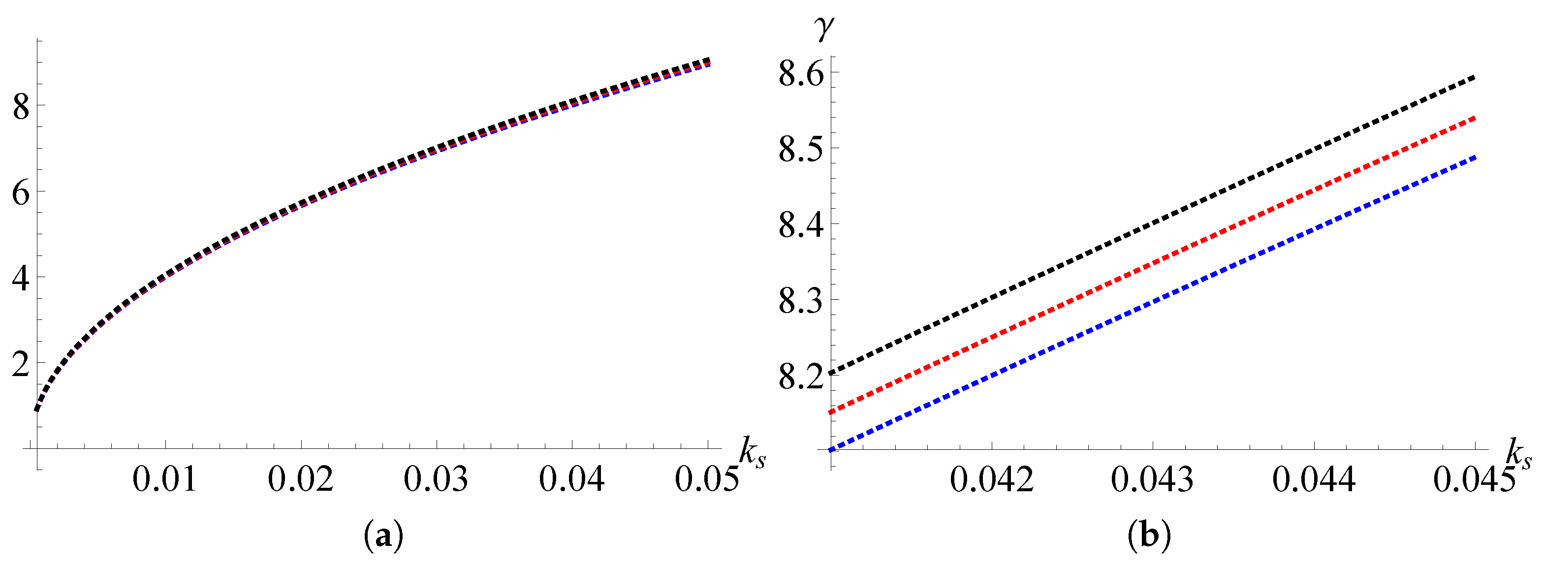
Now, we can analyze the effects of the system parameters and on the critical velocity. In Figure 1, the effects of on the have been plotted. It shows that the first three critical velocity are almost identical when the parameter is very large. In addition, it appears that the relation between critical velocity and nonlocal parameter is linear.
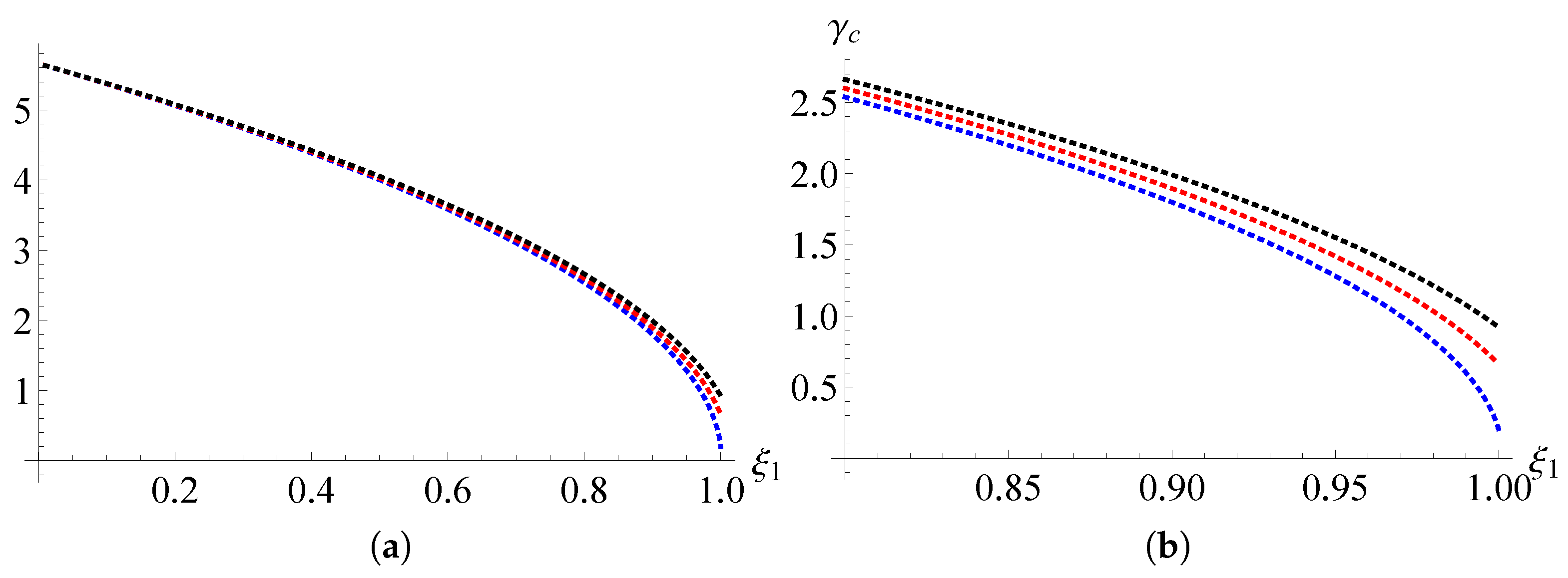
The effect of the volume fraction on the first three critical velocity is plotted in Figure 2, from which we find that the difference between the critical velocities for the first three modes decreases with the decreasing of the volume fraction .
In Figure 3, the effect of the geometric parameter on the critical velocity of the axially moving beam is plotted. We see that the critical velocity increases with the growth of the parameter for both the nonlocal beam and the classical beam. From Figure 3, we find that the critical velocity is almost identical for the first three modes. However, the critical velocity increases with the growth of the mode number k. Furthermore, the critical velocity of the nonlocal beam is always much larger than that of the classical beam (Figure 3a).
We can determine the critical velocity for the fixed boundary by a similar procedure. The critical velocity in this case can be determined by the following equation:
The effects of parameters and on the critical velocity are obtained by the numerical method. The results are plotted in the following Figure 4, Figure 5 and Figure 6. From these figures, we find that the difference of critical velocity between the results of simply supported boundary condition and the fixed boundary condition is very small. In other words, it implies that the critical velocity is almost independent of the boundary conditions for the axially moving beam.
3.2. Natural Frequencies
The mode functions and natural frequencies of axially moving nanobeam can be determined from the corresponding linear equation of the governing Equation (9). After linearizing Equation (9), mode functions and natural frequencies can be determined by the following equation
The general solutions to Equation (22) can be written as
where is the n-th natural frequency and is the mode function.
Substituting Equation (23) into Equation (22), we obtain
It is easy to know that the solution of Equation (24) can be written as
where are constants to be determined and are the roots of the following equation
Firstly, we consider the natural frequencies of beam under simply supported boundary condition. To this end, after substituting Equation (25) into boundary condition Equation (12), a linear algebraic system for can be obtained as
For non-trivial solutions, the determinant D of the coefficient matrix of Equation (27) must be zero. Here, the long expression of D have been omitted for brevity. The natural frequencies and can be solved numerically from Equation (26) and .
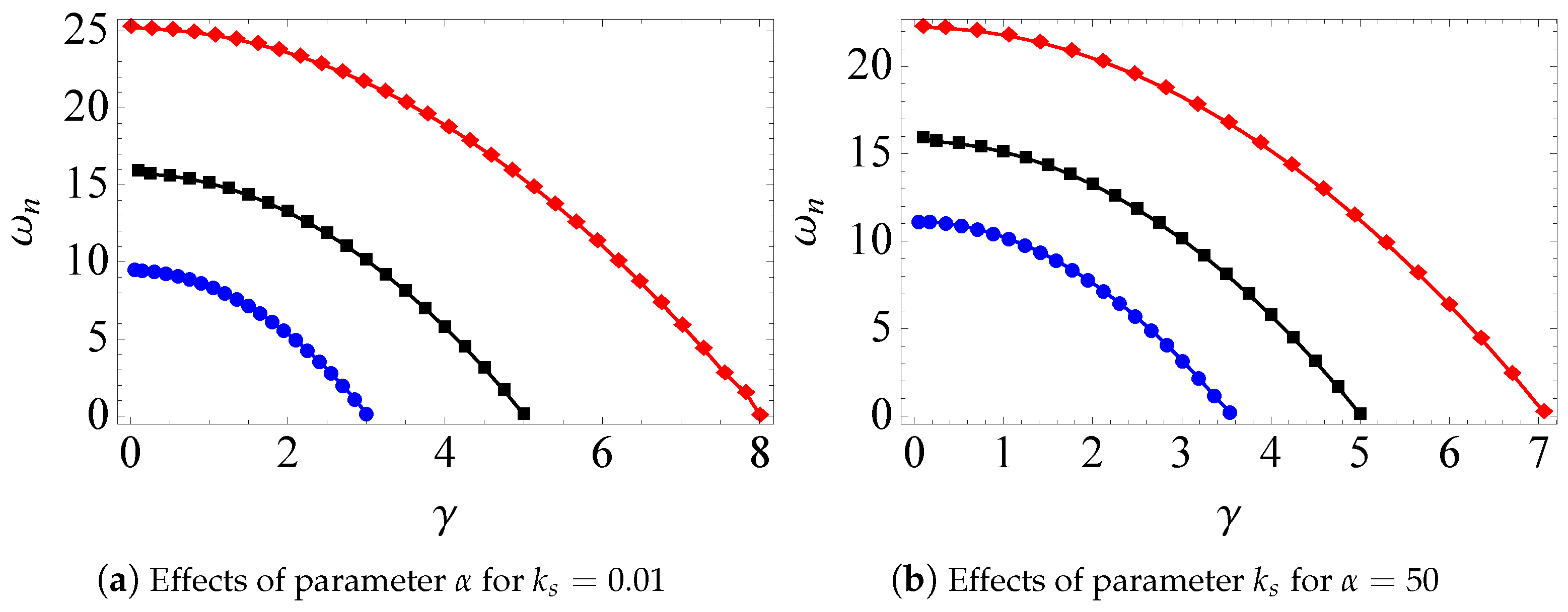
Effects of the nonlocal parameter , volume fraction and geometrical parameter on the natural frequency are shown in Figure 7 and Figure 8. The size effect on the first model of natural frequency of the axially moving nonlocal beam is shown in Figure 7a. It shows that the natural frequency increases with the increase of nonlocal parameter .
In Figure 7b, the effect of parameter on the natural frequency of the first mode is shown. It shows that the natural frequency also increases with the increase of .
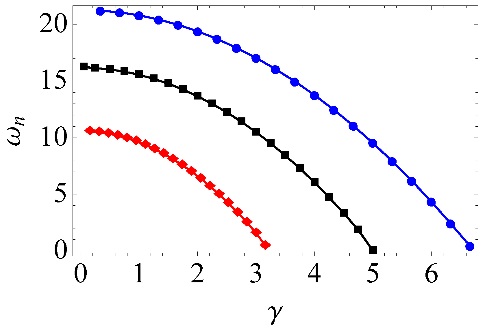
In Figure 8, the effect of parameter on the natural frequency of the first mode is shown. It can be seen that the natural frequency decreases with the increase of . It indicates that the integral model will cause larger natural frequency for nanobeams.
Now, we consider the natural frequency for the case of fixed boundary condition. In this case, the linear Equation (27) can be rewritten as
Similarly, the effects of the parameters and on the natural frequencies can be obtained by numerical method and the results are plotted in the Figure 9 and Figure 10.
From these two figures, we find that the parameters have similar effects on the natural frequencies as those of simply supported boundary condition. However, the natural frequencies of the beam under fixed boundary condition is larger than that of a simply supported boundary condition.
4. Conclusions
In this paper, for the axially moving nanobeams, Eringen’s two-phase nonlocal model is adopted. The integral governing equations for the corresponding nonlinear vibration with simple supported and fixed boundary conditions are obtained by Hamilton’s Principle. The dispersion relation and a characteristic equation are obtained for the free vibration. The critical velocity of the nanobeams are also obtained. The results show that the nonlocal parameter plays a very important role in determining the critical velocity. As for natural frequency, we find that it increases with the increasing of the nonlocal parameter . However, an increase in the volume fraction will reduce the natural frequency.
Author Contributions
Conceptualization, Y.W., X.Z.; Methodology, Y.W., Z.L.; Software, Y.W., K.H.; Writing—Original Draft Preparation, Y.W., X.Z.; Writing—Review & Editing, Z.L., K.H.; Funding Acquisition, Z.L., Y.W.
Funding
This work is supported by the Natural Science Foundation of China (Nos. 11472177, 11422214, 11501578) and the Natural Science Foundation of Zhejiang Province (No. LY19A020005).
Conflicts of Interest
The authors declare no conflict of interest.
References
- Hu, D.; Tang, Y.T.; Chen, L.Q. Frequencies of transverse vibration of an axially moving viscoelastic beam. J. Vib. Control 2015. [Google Scholar] [CrossRef]
- Wickert, J.A. Non-linear vibration of a traveling tensioned beam. Int. J. Nonlinear Mech. 1992, 27, 503–517. [Google Scholar] [CrossRef]
- Ghayesh, M.H.; Amabili, M. Nonlinear dynamics of an axially moving Timoshenko beam with an internal resonance. Nonlinear Dyn. 2013, 73, 39–52. [Google Scholar] [CrossRef]
- Hu, D.; Chen, L.Q. Galerkin methods for natural frequencies of high-velocity axially moving beams. J. Sound Vib. 2010, 329, 3484–3494. [Google Scholar]
- Ghayesh, M.H.; Amabili, M.; Farokhi, H. Global dynamics of an axially moving buckling beam. J. Vib. Control 2015, 21, 195–208. [Google Scholar] [CrossRef]
- Challamel, N.; Wang, C.M. The small length scale effect for a non-local cantilever beam: A paradox solved. Nanotechnology 2008, 19, 345703. [Google Scholar] [CrossRef] [PubMed]
- Eringen, A.C. On differential equations of nonlocal elasticity and solutions of screw dislocation and surface waves. J. Appl. Phys. 1983. [Google Scholar] [CrossRef]
- Reddy, J.N. Nonlocal theories for bending, buckling and vibration of beams. Int. J. Eng. Sci. 2007, 45, 288–307. [Google Scholar] [CrossRef]
- Reddy, J.N.; Pang, S.D. Nonlocal continuum theories of beams for the analysis of carbon nanotubes. J. Appl. Phys. 2007, 103. [Google Scholar] [CrossRef]
- Lim, C.W.; Zhang, G.; Reddy, J.N. A higher-order nonlocal elasticity and strain gradient theory and its applications in wave propagation. J. Mech. Phys. Solids 2007, 78, 298–313. [Google Scholar] [CrossRef]
- Kiani, K. Longitudinal, transverse and torsional vibrations and stabilities of axially moving single-walled carbon nanotubes. Curr. Appl. Phys. 2013, 13, 1651–1660. [Google Scholar] [CrossRef]
- Rezaee, M.; Lotfan, S. Non-linear nonlocal vibration and stability analysis of aixally moving nanoscale beams with time-dependent velocity. Int. J. Mech. Sci. 2015, 96, 36–46. [Google Scholar] [CrossRef]
- Lim, C.W.; Li, C.; Yu, J.L. Dynamic behaviour of axially moving nanobeams based on nanolocal elasticity approach. Acta Mech. Sin.-PRC 2010, 26, 755–765. [Google Scholar] [CrossRef]
- Li, C. Nonlocal Thermo-Electro-Mechanical coupling vibrations of axially moving piezoelectric nanobeams. Mech. Based Des. Struct. 2017, 45, 463–478. [Google Scholar] [CrossRef]
- Liu, J.J.; Li, C. Dynamical responses and stabilities of axially moving nanoscale beams with time-dependent velocity using a nonlocal stress gradient theory. J. Vib. Control 2016. [Google Scholar] [CrossRef]
- Wang, J.; Shen, H.M. Complex modal analysis of transverse free vibrations for axially moving nanobeams based on the nonlocal strain gradient theory. Physica E 2018, 101, 85–93. [Google Scholar] [CrossRef]
- Fernández-Sáez, J.; Zaera, R.; Loya, J.A.; Reddy, J.N. Bending of Euler-Bernoulli beams using Eringen’s integral formulation: A paradox resolved. Int. J. Eng. Sci. 2016, 99, 107–116. [Google Scholar] [CrossRef]
- Tuna, M.; Kirca, M. Exact solutions of Eringen’s nonlocal integral model for bending of Euler-Bernoulli and Timoshenko beams. Int. J. Eng. Sci. 2016, 105, 80–92. [Google Scholar] [CrossRef]
- Romano, G.; Barretta, R.; Diaco, M.; Sciarra, F.M.D. Constitutive boundary conditions and paradoxes in nonlocal elastic nanobeams. Int. J. Mech. Sci. 2016, 121, 151–156. [Google Scholar] [CrossRef]
- Li, C.; Yao, L.Q.; Chen, W.Q.; Li, S. Comments on nonlocal effects in nano-cantilever beams. Int. J. Eng. Sci. 2015, 87, 47–57. [Google Scholar] [CrossRef]
- Barretta, R.; Feo, L.; Luciano, R.; Diaco, M.; Sciarra, F.M.D. Application of an enhanced version of the Eringen differential model to nanotechnology. Compos. Part B-Eng. 2016, 96, 274–280. [Google Scholar] [CrossRef]
- Romano, G.; Barretta, R.; Diaco, M. On nonlocal integral models for elastic nano-beams. Int. J. Mech. Sci. 2017, 131–132, 490–499. [Google Scholar] [CrossRef]
- Romano, G.; Luciano, R.; Barretta, R.; Diaco, M. Nonlocal integral elasticity in nanostructures, mixtures, boundary effects and limit behaviours. Continuum Mech. Therm. 2018, 30, 641–655. [Google Scholar] [CrossRef]
- Wang, Y.B.; Zhu, X.W.; Dai, H.H. Exact solutions for the static bending of Euler-Bernoulli beams using Eringen’s two-phase local/nonlocal model. AIP Adv. 2016, 6. [Google Scholar] [CrossRef]
- Zhu, X.W.; Wang, Y.B.; Dai, H.H. Buckling analysis of Euler-Bernoulli beams using Eringen’s two-phase nonlocal model. Int. J. Eng. Sci. 2017, 116, 130–140. [Google Scholar] [CrossRef]
- Fernández-Sáez, J.; Zaera, R. Vibrations of Bernoulli-Euler beams using the two-phase nonlocal elasticity theory. Int. J. Eng. Sci. 2017, 119, 232–248. [Google Scholar] [CrossRef]
- Romano, G.; Barretta, R. Nonlocal elasticity in nanobeams: The stress-driven integral model. Int. J. Eng. Sci. 2017, 115, 14–27. [Google Scholar] [CrossRef]
- Romano, G.; Barretta, R. Stress-driven versus strain-driven nonlocal integral model for elastic nano-beams. Compos. Part B-Eng. 2017, 114, 184–188. [Google Scholar] [CrossRef]
- Barretta, R.; Diaco, M.; Feo, L.; Luciano, R.; Sciarra, F.M.D.; Penna, R. Stress-driven integral elastic theory for torsion of nano-beams. Mech. Res. Commun. 2018, 87, 35–41. [Google Scholar] [CrossRef]
- Barretta, R.; Ali Faghidian, S.; Luciano, R.; Medaglia, C.M.; Penna, R. Stress-driven two-phase integral elasticity for torsion of nano-beams. Compos. Part B-Eng. 2018, 145, 62–69. [Google Scholar] [CrossRef]
- Barretta, R.; Čanadija, M.; Luciano, R.; Sciarra, F.M.D. Stress-driven modeling of nonlocal thermoelastic behavior of nanobeams. Int. J. Eng. Sci. 2018, 126, 53–67. [Google Scholar] [CrossRef]
Figure 1.
The critical velocity versus nonlocal parameter when and . Black dotted line, red dotted line and blue dotted line denote the results for mode, respectively. (a) full graph, (b) enlarger partial of full graph.
Figure 1.
The critical velocity versus nonlocal parameter when and . Black dotted line, red dotted line and blue dotted line denote the results for mode, respectively. (a) full graph, (b) enlarger partial of full graph.

Figure 2.
The critical velocity versus volume fraction when . Black dotted line, red dotted line and blue dotted line denote the results for mode, respectively. (a) full graph, (b) enlarger partial of full graph.
Figure 2.
The critical velocity versus volume fraction when . Black dotted line, red dotted line and blue dotted line denote the results for mode, respectively. (a) full graph, (b) enlarger partial of full graph.

Figure 3.
The critical velocity versus geometric parameter when . Black dotted line, red dotted line and blue dotted line denote the results for mode, respectively. In (a), the bottom of the three dotted lines denote the critical velocity of the classical results. (b) enlarger partial of full graph for nonlocal model.

Figure 4.
The critical velocity versus geometric parameter when under fixed boundary condition. Black dotted line, red dotted line and blue dotted line denote the results for mode, respectively. (a) full graph, (b) enlarger partial of full graph.
Figure 4.
The critical velocity versus geometric parameter when under fixed boundary condition. Black dotted line, red dotted line and blue dotted line denote the results for mode, respectively. (a) full graph, (b) enlarger partial of full graph.

Figure 5.
The critical velocity versus geometric parameter when . Black dotted line, red dotted line and blue dotted line denote the results for mode, respectively. (a) full graph, (b) enlarger partial of full graph.
Figure 5.
The critical velocity versus geometric parameter when . Black dotted line, red dotted line and blue dotted line denote the results for mode, respectively. (a) full graph, (b) enlarger partial of full graph.

Figure 6.
The critical velocity versus geometric parameter when . Black dotted line, red dotted line and blue dotted line denote the results for mode, respectively. (a) full graph, (b) enlarger partial of full graph.
Figure 6.
The critical velocity versus geometric parameter when . Black dotted line, red dotted line and blue dotted line denote the results for mode, respectively. (a) full graph, (b) enlarger partial of full graph.

Figure 7.
The natural frequency for different and , with fixed. (a) from top to bottom ; (b) from top to bottom .
Figure 7.
The natural frequency for different and , with fixed. (a) from top to bottom ; (b) from top to bottom .

Figure 8.
The natural frequency for different with fixed, from top to bottom .

Figure 9.
The natural frequency for different and , with fixed. (a) from top to bottom ; (b) from top to bottom .
Figure 9.
The natural frequency for different and , with fixed. (a) from top to bottom ; (b) from top to bottom .

Figure 10.
The natural frequency for different with fixed, from top to bottom .

© 2018 by the authors. Licensee MDPI, Basel, Switzerland. This article is an open access article distributed under the terms and conditions of the Creative Commons Attribution (CC BY) license (http://creativecommons.org/licenses/by/4.0/).
Share and Cite
MDPI and ACS Style
Wang, Y.; Lou, Z.; Huang, K.; Zhu, X. Size-Dependent Free Vibration of Axially Moving Nanobeams Using Eringen’s Two-Phase Integral Model. Appl. Sci. 2018, 8, 2552. https://doi.org/10.3390/app8122552
AMA Style
Wang Y, Lou Z, Huang K, Zhu X. Size-Dependent Free Vibration of Axially Moving Nanobeams Using Eringen’s Two-Phase Integral Model. Applied Sciences. 2018; 8(12):2552. https://doi.org/10.3390/app8122552
Chicago/Turabian StyleWang, Yuanbin, Zhimei Lou, Kai Huang, and Xiaowu Zhu. 2018. "Size-Dependent Free Vibration of Axially Moving Nanobeams Using Eringen’s Two-Phase Integral Model" Applied Sciences 8, no. 12: 2552. https://doi.org/10.3390/app8122552
Note that from the first issue of 2016, this journal uses article numbers instead of page numbers. See further details here.