An Observer-Based Active Fault Tolerant Controller for Vehicle Suspension System

Abstract

This paper proposes an observer-based active fault-tolerant controller for a half-vehicle active suspension system subjected to the actuator fault as the nonzero offset fault. By constructing the augmented fault suspension system model, an H_∞ weighted output feedback controller was developed to improve the vehicle dynamics performances under a fault-free condition. Moreover, a robust observer was designed to make an accurate estimation of the fault information with the auxiliary diagnosis system and further to develop an H_∞ fault compensation controller, such that the closed-loop control system can eliminate the negative effects of the actuator faults on vehicle suspension performances. Finally, a numerical simulation investigation was provided to verify the effectiveness of the proposed controller under the random and bump road disturbances.

1. Introduction

Over the past decades, vehicle suspension design has become an important research topic due to their attribution to improving ride comfort and handling stability of the vehicle body. Generally, the suspension system can be categorized into three types as passive suspension, semi-active suspension, and active suspension systems [1,2]. Passive suspensions comprise springs and dampers installed between the vehicle body and the wheel axle, which can achieve good ride comfort or good road holding since these two criteria conflict with each other. Semi-active suspensions can offer better improvement by adjusting their variable damping coefficients and just needs lower power consumption. It should be noted that electrorheological and magnetorheological fluid dampers are usually preferred in semi-active suspension systems. In the active suspension system, an additional actuator (linear motor, hydraulic cylinder, etc.) is installed to suppress its vibrations caused by the road irregularities. As compared with the passive suspension, the semi-active and active suspension are more easily combined with the advanced control algorithms such as H_∞ control [3,4], sliding-mode control [5], adaptive backstepping control [6,7], T-S fuzzy control [8,9], and nonlinear control [10,11], wherein a good trade-off between the two conflicting suspension performances as ride quality and handling stability can be made. However, these control schemes are all based on the assumption that all of the components of vehicle suspension system work under the non-fault model, which is inconsistent with the actual application scenario [12,13] in some ways. With the growing demand for safety, reliability, and maintainability in the vehicle suspension system, it is necessary to develop a comprehensive fault-tolerant control (FTC) scheme to maintain a desirable system performance whether there occurs a fault in active suspension system or not.

It is well demonstrated in the previous studies [14,15] that FTC possesses the ability to accommodate failures automatically and then maintains a stability and sufficient level of system performance. In general, there are two types of fault-tolerant control approaches named as the passive and active ones. It should be noted that these two fault-tolerant control methods usually employ different design methodologies for the same control plants and will result in some unique properties. On the one side, for the development of the passive FTC scheme, a robust controller is often designed to deal with all the underlying faults. For instance, the authors in [16] proposed a sliding mode fault-tolerant control scheme for a nonlinear system guaranteeing the asymptotic stability of the control system under faults, yet it still possessed disadvantages like large chattering, which imposes some restrictions in its practical applications. In addition to this, a robust H_∞ fault tolerant controller was developed to maintain the stability and constraint performance of an active suspension system with the bounded actuator faults [17]. Moreover, some related research can also be found in [18,19]. Specifically, an adaptive fault tolerant controller is proposed in [20] for an active suspension system with unknown actuator faults, which ensures the boundedness of the vertical and pitch angle displacements. It was noted that the aforementioned passive FTC approaches were only reliable for the specific system faults encountered in the system operation, wherein the designed FTC may not possess a better control performance under all kinds of faults.

On the other hand, when designing active FTC schemes, it is usually aimed at ensuring the system stability with an acceptable constraint performance by reconfiguring the on-line controller with the fault detection and diagnosis (FDD) system, which can estimate and compensate for the system fault and has been used in many areas [21,22,23,24,25,26,27]. In [25], a specific actuator failure for the three-tank system was first detected and confirmed by a fault diagnosis unit, the control law was then reconfigured based on the information of the detected fault. Both the stability and the acceptable H_∞ disturbance attenuation level were guaranteed for the closed-loop system using the remaining reliable actuators. Besides, a new FTC algorithm for an automotive air suspension control system has been developed in [26], where the fault detection, diagnosis, and management of a closed-loop air suspension control system are included to enhance the robustness of the fault detection and isolation against uncertainties. However, only the height sensor faults are considered and it is of high cost in practical engineering applications. The authors in [27] developed an FTC algorithm for vehicle active suspension systems in finite-frequency with a sine wave input fault and a new H_∞ FTC controller was developed based on a GIMC (Generalized Internal Mode Control) structure by ignoring the design of the fault diagnosing system. However, the fault model is less convincing and hard to be applied in reality. Thus, it is still a challenging issue to make the related FTC scheme in the active suspension system.

Motivated by the aforementioned research and discussion, this paper investigates the problem of observer-based active fault-tolerant control design for a half-vehicle active suspension system subjected to the actuator fault as the nonzero offset fault. The system augmentation technique and Lyapunov stability theory were introduced to design the fault tolerant controller. The key contributions of this work are summarized as follows.

First, a comprehensive control scheme of active fault tolerant controller was constructed for an active suspension system, which can not only deal with the desirable performance control for active suspension system without the actuator faults, but also achieve a way for ensuring the system performance when actuator faults occur.

Second, a robust observer was designed to make an accurate estimation of the fault information with the auxiliary diagnosis system and to further develop an H_∞ fault compensation controller, such that the closed-loop control system can eliminate the negative effects of the actuator faults on vehicle suspension performances.

Finally, some illustrative examples were provided to demonstrate the validity of the control scheme proposed in this paper.

The rest of this paper is organized as follows: Section 2 presents system modeling problem formulation for active suspension system with the general faults. The proposed robust observer-based active fault-tolerant controller design is presented in Section 3. In Section 4, the simulation investigation is provided to demonstrate the effectiveness of the designed controller. The conclusions are given in Section 5.

2. System Modelling and Problem Statement

2.1. Generalized Fault Model of Active Suspension System

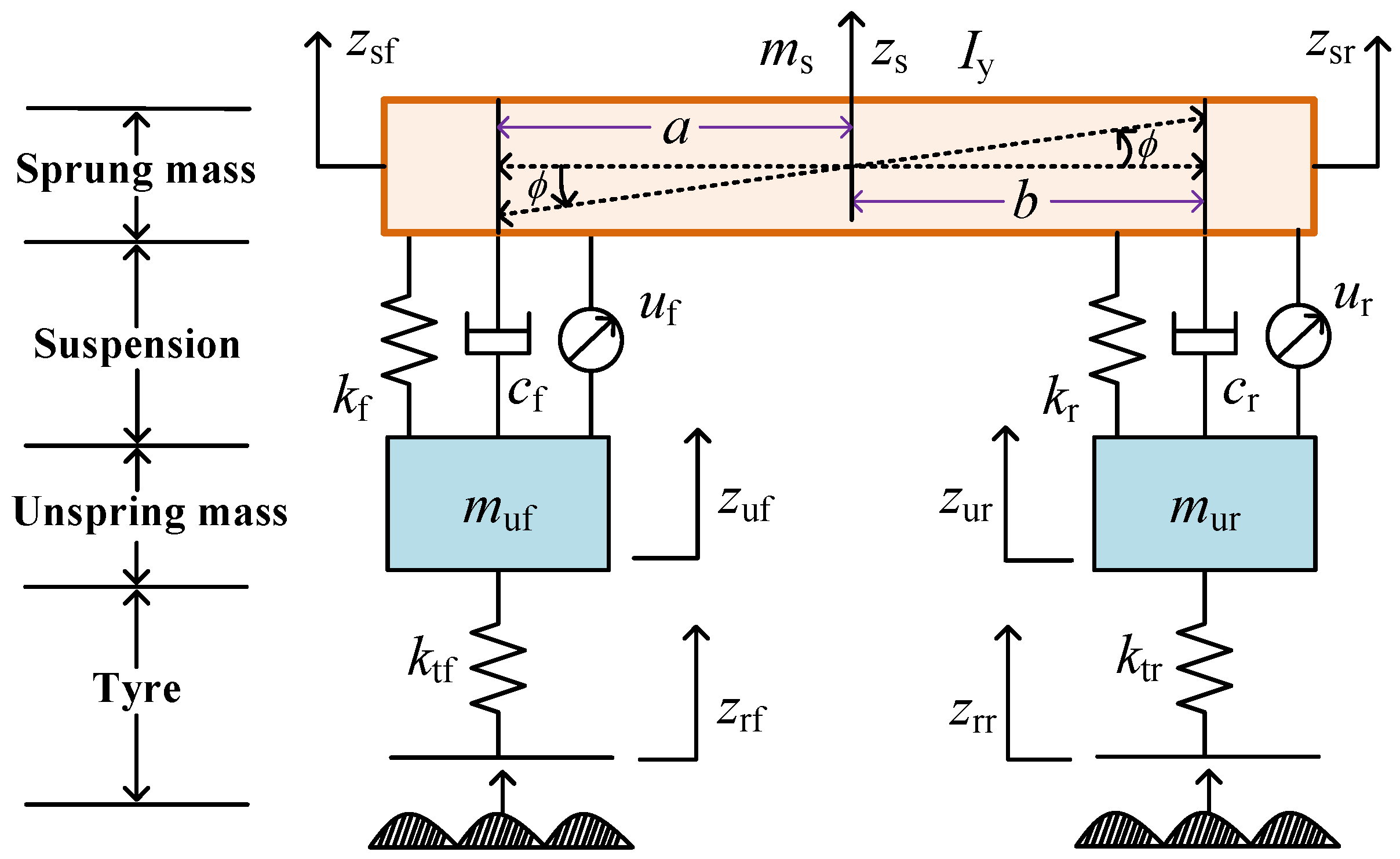
A half-vehicle suspension model with four DOFs (degree-of-freedoms) is shown in Figure 1, in which, m_s an I_y denote the sprung mass and its moment of inertia, z_s and $\phi$ denote the vertical and pitch angular displacement at the center gravity (CG) of the vehicle body, respectively; a and b denote the horizontal distances from the CG of the vehicle body to the front and rear axles, respectively; m_uf and m_ur denote the unsprung mass of the front and rear suspension, respectively; c_f and c_r represent the damping coefficients of the front and rear suspension, respectively; k_f and k_r represent the stiffness coefficients of the front and rear suspension, respectively; z_si, z_ui, and z_ri (i = f, r, stands for the front and rear suspension) denote the suspension vertical displacements of the sprung and unsprung mass, and the road disturbance inputs to the front and rear wheels, respectively; u_f and u_r represent the control forces of the front and rear suspension, respectively. Ignoring the damping characteristics of tires, k_tf and k_tr denote the tire stiffness coefficients of the front and rear wheels, respectively.

It was assumed that the front and rear wheels had the same road excitation signals, thus the vertical displacements of the front and rear suspension sprung masses had the following relationship with a smaller pitch angular $\phi$ as [28]

$$\{\begin{array}{c}{z}_{\mathrm{sf}}\cong z_{\mathrm{s}}-a\sin \varphi \approx z_{\mathrm{s}}-a\varphi \\ z_{\mathrm{sr}}\cong z_{\mathrm{s}}+b\sin \varphi \approx z_{\mathrm{s}}+b\varphi \end{array}$$

(1)

Based on Newton’s second law, the dynamics equations of the half-vehicle suspension system was written as follows:

$$\{\begin{array}{l}{m}_{\mathrm{s}}{\ddot{z}}_{\mathrm{s}}=-k_{\mathrm{f}}(z_{\mathrm{sf}}-z_{\mathrm{uf}})-c_{\mathrm{f}}({\dot{z}}_{\mathrm{sf}}-{\dot{z}}_{\mathrm{uf}})-k_{\mathrm{r}}(z_{\mathrm{sr}}-z_{\mathrm{ur}})-c_{\mathrm{r}}({\dot{z}}_{\mathrm{sr}}-{\dot{z}}_{\mathrm{ur}})+u_{\mathrm{f}}+u_{\mathrm{r}}\\ I_{\mathrm{y}}\ddot{\varphi }=-a{k}_{\mathrm{f}}(z_{\mathrm{sf}}-z_{\mathrm{uf}})-a{c}_{\mathrm{f}}({\dot{z}}_{\mathrm{sf}}-{\dot{z}}_{\mathrm{uf}})+b{k}_{\mathrm{r}}(z_{\mathrm{sr}}-z_{\mathrm{ur}})+b{c}_{\mathrm{r}}({\dot{z}}_{\mathrm{sr}}-{\dot{z}}_{\mathrm{ur}})+a{u}_{\mathrm{f}}-b{u}_{\mathrm{r}}\\ m_{\mathrm{uf}}{\ddot{z}}_{\mathrm{uf}}=k_{\mathrm{f}}(z_{\mathrm{sf}}-z_{\mathrm{uf}})+c_{\mathrm{f}}({\dot{z}}_{\mathrm{sf}}-{\dot{z}}_{\mathrm{uf}})-k_{\mathrm{tf}}(z_{\mathrm{uf}}-z_{\mathrm{rf}})-u_{\mathrm{f}}\\ m_{\mathrm{ur}}{\ddot{z}}_{\mathrm{ur}}=k_{\mathrm{r}}(z_{\mathrm{sr}}-z_{\mathrm{ur}})+c_{\mathrm{r}}({\dot{z}}_{\mathrm{sr}}-{\dot{z}}_{\mathrm{ur}})-k_{\mathrm{tr}}(z_{\mathrm{ur}}-z_{\mathrm{rr}})-u_{\mathrm{r}}\end{array}$$

(2)

Define the state vector as $\mathit{x}\left(t\right)={\left[z_{\mathrm{s}},{\dot{z}}_{\mathrm{s}},\phi ,\dot{\phi },z_{\mathrm{uf}},z_{\mathrm{ur}},{\dot{z}}_{\mathrm{uf}},{\dot{z}}_{\mathrm{ur}}\right]}^T$, the disturbance input as $\mathit{d}\left(t\right)={[z_{\mathrm{rf}},z_{\mathrm{rr}}]}^T$, the control input as $\mathit{u}\left(t\right)={\left[u_{\mathrm{f}}{,u}_{\mathrm{r}}\right]}^T$, the control output as $\mathit{z}\left(t\right)={\left[{\ddot{z}}_{\mathrm{s}},\ddot{\phi }{,z}_{\mathrm{sf}}-z_{\mathrm{uf}}{,z}_{\mathrm{sr}}-z_{\mathrm{ur}}{,u}_{\mathrm{f}}{,u}_{\mathrm{r}}\right]}^T$, and the measured output as $\mathit{y}\left(t\right)={\left[{\dot{z}}_{\mathrm{s}},\dot{\phi }{,z}_{\mathrm{sf}}-z_{\mathrm{uf}}{,z}_{\mathrm{sr}}-z_{\mathrm{ur}}\right]}^T$, wherein ${\ddot{z}}_{\mathrm{s}}$ and $\ddot{\phi }$ represent the vertical and pitch angular accelerations of the vehicle body, respectively; ${\dot{z}}_{\mathrm{s}}$ and $\dot{\phi }$ represent the vertical and pitch angular velocities of the vehicle body, respectively; $z_{\mathrm{sf}}-z_{\mathrm{uf}}$ and $z_{\mathrm{sr}}-z_{\mathrm{ur}}$ represent the dynamic deflections of the front and rear suspension, respectively. Then, the system state-space equation of half-vehicle suspension was given by

$$\{\begin{array}{l}\dot{\mathit{x}}(t)=\mathit{A}\mathit{x}(t)+\mathit{B}\mathit{u}(t)+{\mathit{B}}_d\mathit{d}(t)\\ \mathit{y}(t)={\mathit{C}}_1\mathit{x}(t)\\ \mathit{z}(t)={\mathit{C}}_2\mathit{x}(t)+{\mathit{D}}_2\mathit{u}(t)\end{array}$$

(3)

where A, B, B_d, C₁, C₂, and D₂ were the matrices with appropriate dimensions to be determined, which are expressed in Appendix A.

It is widely accepted that the fault has the characteristic of randomness, fuzziness, and unpredictability. The common faults like actuator jam or offset in sensor outputs were firstly tested in the experiment bench and were then modeled in a finite parameter family as a constant gain fault or slow drift fault [29]. Without loss of generality, the following exosystem was used to describe the actuator fault model as [30,31]

$$\{\begin{array}{l}{\dot{\mathit{x}}}_f(t)={\mathit{A}}_{wf}{\mathit{x}}_f(t)+{\mathit{B}}_{wf}\mathit{\delta }(t)\hfill \\ \mathit{f}(t)={\mathit{C}}_{wf}{\mathit{x}}_f(t)\hfill \end{array}$$

(4)

where x_f $\in R^{n_f}$ denotes the state vector of the fault model, δ(t) denotes the virtual input signal with the bounded L₂ norm. It should be noted that the auxiliary fault diagnosis system was needed to confirm the value of the coefficient matrix and δ(t). In brief, this paper adopted the random ramp signal to describe the actuator fault f(t). Let the coefficient matrix be A_wf = 0, B_wf = I, C_wf = I and δ(t) satisfying:

$$\delta (t)=\{\begin{array}{l}0,t<t_f\\ {\beta }_f,t\ge t_f\end{array}$$

(5)

where t_f and β_f stand for the occurring time and the amplitude of the suspension fault. It is noted that an arbitrarily random ramp signal could be generated by tuning the value of t_f and β_f.

Combining (3) and (4) yields the state-space equations of the half-vehicle suspension system with the generalized actuator faults as:

$$\{\begin{array}{l}\dot{\mathit{x}}(t)=\mathit{A}\mathit{x}(t)+\mathit{B}\mathit{u}(t)+{\mathit{B}}_d\mathit{d}(t)+{\mathit{B}}_f\mathit{f}(t)\\ \mathit{y}(t)={\mathit{C}}_{1}x(t)\\ \mathit{z}\left(t\right)={\mathit{C}}_{2}x(t)+{\mathit{D}}_{2}u(t)+{\mathit{D}}_{2f}\mathit{f}(t)\end{array}$$

(6)

where B_f and D_2f are the known matrices with appropriate dimensions, and there exists a known gain matrix M satisfying [${\mathit{B}}_f^T$ ${\mathit{D}}_{2f}^T$]^T = [${\mathit{B}}^T$ ${\mathit{D}}_2^T$]^TM [26]. It is noted that when f(t) = 0, the active suspension system works under normal operations, and when f(t) ≠ 0, it can be confirmed that there occurs some actuator faults in the active suspension system.

2.2. Problem Statement of Active Fault-Tolerant Control

For the active suspension system in (6), our main objective was to develop a fault-tolerant controller to improve the vehicle dynamics performance in the presence of the actuator faults and the external road disturbance. The proposed control scheme for this active suspension system is shown in Figure 2.

As shown in Figure 2, when the system (6) has no fault, that is, f(t) = 0, the H_∞ output feedback controller works as the proposed active FTC scheme, which can guarantee a better control performance of vehicle suspension system. When there are some systematic faults in (6), i.e., f(t) ≠ 0, the proposed active FTC scheme is composed of the H_∞ output feedback controller and H_∞ observer-based fault compensation controller, in which the fault compensation controller is employed to observe and estimate the fault information and further, to design the fault compensative control law to eliminate the effects of the faults on vehicle suspension system performances. At the same time, the H_∞ output feedback controller starts to work so as to ensure that the closed-loop system is stable and robust to the external disturbance inputs. In this control scheme, both of the fault compensation controller and robust H_∞ output feedback controller work together to achieve the active fault-tolerant control for active suspension system (6).

To sum up, the designed active fault-tolerant controller is formed as:

$$\mathit{u}(t)={\mathit{u}}_N(t)+{\mathit{u}}_C(t)$$

(7)

where u_N(t) is the control law of H_∞ output-feedback controller, and u_C(t) is the control law of fault compensation controller.

Substituting (7) into (6) gives the closed-loop system as:

$$\{\begin{array}{l}\dot{\mathit{x}}(t)=\mathit{A}\mathit{x}(t)+\mathit{B}{\mathit{u}}_N(t)+\mathit{B}{\mathit{u}}_C(t)+{\mathit{B}}_d\mathit{d}(t)+{\mathit{B}}_f\mathit{f}(t)\\ \mathit{y}(t)={\mathit{C}}_1\mathit{x}(t)\\ \mathit{z}(t)={\mathit{C}}_2\mathit{x}(t)+{\mathit{D}}_2{\mathit{u}}_N(t)+{\mathit{D}}_2{\mathit{u}}_C(t)+{\mathit{D}}_{2f}\mathit{f}(t)\end{array}$$

(8)

Therefore, the control objective in this article can be defined as: For the system (8), one can design u_C(t) = $-\mathit{M}\widehat{\mathit{f}}(t)$ to make Bu_C(t) + B_ff(t) = 0, and D₂u_C(t) + D_2ff(t) = 0, thus to compensate for the performance penalties caused by the actuator faults. Moreover, the control law u_N(t) = K(s)y(t) is designed to ensure the asymptotic stability of the closed-loop system (8). It should be noted here that $\widehat{\mathit{f}}(t)$ is the estimation of f(t).

To fulfill the fault estimation and compensation, substituting (4) into (6) yields the following augmented system as:

$$\{\begin{array}{l}\dot{\mathit{\varsigma }}(t)={\mathit{A}}_{ef}\mathit{\varsigma }(t)+{\mathit{B}}_{ef}\mathit{u}(t)+{\mathit{F}}_e\mathit{w}(t)\\ \mathit{y}(t)={\mathit{C}}_e\mathit{\varsigma }(t)\\ \mathit{f}(t)={\mathit{C}}_{ef}\mathit{\varsigma }(t)\end{array}$$

(9)

where

$$\mathit{\varsigma }(t)=\left[\begin{array}{c}\mathit{x}(t)\\ {\mathit{x}}_f(t)\end{array}\right],\mathit{w}(t)=\left[\begin{array}{c}\mathit{d}(t)\\ \mathit{\delta }(t)\end{array}\right],$$

$${\mathit{A}}_{ef}=\left[\begin{array}{cc}\mathit{A}& {\mathit{B}}_f{\mathit{C}}_{wf}\\ \mathbf{0}& {\mathit{A}}_{wf}\end{array}\right],{\mathit{B}}_{ef}=\left[\begin{array}{c}\mathit{B}\\ \mathbf{0}\end{array}\right],$$

$${\mathit{F}}_e=\left[\begin{array}{cc}{\mathit{F}}_{1e}& {\mathit{F}}_{2e}\end{array}\right],{\mathit{F}}_{1e}=\left[\begin{array}{c}{\mathit{B}}_d\\ \mathbf{0}\end{array}\right]{\mathit{F}}_{2e}=\left[\begin{array}{c}\mathbf{0}\\ {\mathit{B}}_{wf}\end{array}\right],$$

$${\mathit{C}}_e=\left[\begin{array}{cc}{\mathit{C}}_1& {\mathit{D}}_{1f}{\mathit{C}}_{wf}\end{array}\right],{\mathit{C}}_{ef}=\left[\begin{array}{cc}\mathbf{0}& {\mathit{C}}_{wf}\end{array}\right].$$

It is assumed that in the augmented system (9), (A_ef, B_ef) is controllable, and (C_ef, A_ef) is measurable, thus an augmented observer can be constructed to detect the system state and fault signal information after the system faults occur, and the full-order state observer of the system (9) is then expressed as:

$$\{\begin{array}{l}\dot{\widehat{\mathit{\varsigma }}}(t)={\mathit{A}}_{ef}\stackrel{⌒}{\mathit{\varsigma }}(t)+{\mathit{B}}_{ef}u(t)+\mathit{L}(\mathit{y}(t)-{\mathit{C}}_e\widehat{\mathit{\varsigma }}(t))\\ \stackrel{⌒}{\mathit{f}}(t)={\mathit{C}}_{ef}\widehat{\mathit{\varsigma }}(t)\end{array}$$

(10)

where $\widehat{\mathit{\varsigma }}(t)\in R^{n+n_f}$ and L are the state vector and gain matrix for the augmented observer, respectively.

Let

$$\mathit{e}(t)=\mathit{\varsigma }(t)-\stackrel{⌒}{\mathit{\varsigma }}(t)$$

(11)

$$\tilde{\mathit{f}}(t)=\mathit{f}(t)-\widehat{\mathit{f}}(t)$$

(12)

From (9) and (10), we have

$$\{\begin{array}{l}\dot{\mathit{e}}(t)=({\mathit{A}}_{ef}-\mathit{L}{\mathit{C}}_e)\mathit{e}(t)+{\mathit{F}}_e\mathit{w}(t)\\ \tilde{\mathit{f}}(t)={\mathit{C}}_{ef}\mathit{e}(t)\end{array}$$

(13)

Synthesizing (8) and (13) gives the active fault-tolerant control system of half-vehicle suspension as follows:

$$\{\begin{array}{l}\dot{\mathit{x}}(t)=\mathit{A}\mathit{x}(t)+\mathit{B}{\mathit{u}}_N(t)+{\mathit{B}}_f{\mathit{C}}_{ef}\mathit{e}(t)+{\mathit{B}}_w\mathit{w}(t)\\ \dot{\mathit{e}}(t)=({\mathit{A}}_{ef}-\mathit{L}{\mathit{C}}_e)\mathit{e}(t)+{\mathit{F}}_e\mathit{w}(t)\\ \mathit{z}(t)={\mathit{C}}_2\mathit{x}(t)+{\mathit{D}}_2{\mathit{u}}_N(t)+{\mathit{D}}_{2f}{\mathit{C}}_{ef}\mathit{e}(t)\end{array}$$

(14)

where B_w = [B_d 0].

Through establishing the augmented system (14), the design of active FTC control scheme can be transformed into solving the gain vector L of the fault observer and the control law u_N(t) of H_∞ output-feedback controller by satisfying the following performance conditions:

(a) The closed-loop system (14) is asymptotically stable.

(b) Under zero initial conditions, $\forall \mathit{w}(t)\in L_2\left[0,+\infty \right)$, supposing that the transfer function from the disturbance input $\mathit{w}(t)$ to the fault error $\tilde{\mathit{f}}(t)$ is $T_{\tilde{f}w}$(s), solving L makes the system (13) satisfying H_∞ performance index ||$T_{\tilde{f}w}$(s)|| < β.

(c) Under zero initial conditions, $\forall \mathit{w}(t)\in L_2\left[0,+\infty \right)$, supposing that the transfer function from the disturbance input $\mathit{w}(t)$ to the control output $\mathit{z}(t)$ is T_zw(s), solving u_N(t)=K(s)y(t) makes the system (13) satisfying ||T_zw(s)||_∞< λ.

To facilitate the following descriptions and our fault-tolerant controller design, Lemma 1 was introduced.

Lemma 1 ([32]).

Consider the following linear time-invariant system

$$\{\begin{array}{l}\mathit{x}(t)=\mathit{A}\mathit{x}(t)+\mathit{B}\mathit{w}(t)\\ \mathit{z}(t)=\mathit{C}\mathit{x}(t)+\mathit{D}\mathit{w}(t)\end{array}$$

(15)

Given a positive constant γ, if there exists a positive definite matrix P > 0 satisfying

$$\left[\begin{array}{ccc}{\mathit{A}}^T\mathit{P}+\mathit{P}\mathit{A}& \mathit{P}\mathit{B}& {\mathit{C}}^T\\ *& -{\gamma }^2\mathit{I}& {\mathit{D}}^T\\ *& *& -\mathit{I}\end{array}\right]$$

(16)

Thus, the system (15) will reach the asymptotical stability and the inequality ||z(t)||₂ < γ||w(t)||₂ holds under zero initial condition.

3. Robust H_∞ Fault-Tolerant Controller Design

From the aforementioned discussions, the proposed active fault-tolerant control scheme was composed of two sub-controllers, that is, the H_∞ weighed output feedback controller and H_∞ observer-based fault compensation controller, which are demonstrated in detail, in this section.

3.1. The Design of H_∞ Fault Compensation Controller

Based on the above discussion in Section 2.2, the proposed H_∞ observer-based fault compensation controller can be summarized as Theorem 1.

Theorem 1.

Consider the full-order state observer of active suspension system in (13), given a positive constant β, if there exist positive matrices P₁ and Y₁ with appropriate dimensions, such that the following linear matrix inequalities (LMIs) hold:

$$\left[\begin{array}{ccc}{\mathit{A}}_{ef}^T{\mathit{P}}_1+{\mathit{P}}_1{\mathit{A}}_{ef}-{\mathit{C}}_e^T{{\mathit{Y}}_1}^T-{\mathit{Y}}_1{\mathit{C}}_e& {\mathit{P}}_1{\mathit{F}}_e-{\mathit{Y}}_1{\mathit{D}}_e& {\mathit{C}}_{ef}^T\\ *& -{\beta }^2\mathit{I}& 0\\ *& *& -\mathit{I}\end{array}\right]<0$$

(17)

Thus, there exists a gain matrix L = P₁⁻¹Y₁ for the designed observer satisfying the following performance conditions:

(a) The closed-loop system (13) is asymptotically stable

(b) Under zero initial conditions, the H_∞ performance index ||$T_{\tilde{f}w}$_(s)|| < β is satisfied.

From Equation (10), the fault compensation control law is designed as:

$$u_C(t)=-M{\mathit{C}}_{ef}\widehat{\varsigma }(t)=-M\widehat{f}(t)$$

(18)

Proof. 

By applying Lemma 1 to the closed-loop system (13), we have:

$$\left[\begin{array}{ccc}{({\mathit{A}}_{ef}-\mathit{L}{\mathit{C}}_e)}^T{\mathit{P}}_1+{\mathit{P}}_1({\mathit{A}}_{ef}-\mathit{L}{\mathit{C}}_e)& {\mathit{P}}_1({\mathit{F}}_e-\mathit{L}{\mathit{D}}_e)& {{\mathit{C}}_{ef}}^T\\ *& -{\beta }^2\mathit{I}& \mathbf{0}\\ *& *& -\mathit{I}\end{array}\right]<0$$

(19)

Based on Lemma 1, the closed-loop system (13) is asymptotically stable and the H_∞ performance index ||$T_{\tilde{f}w}$(s)|| < β is satisfied under a zero initial condition if and only if there exists P₁ > 0 such that inequality (19) holds, and (19) can be further written as:

$$\left[\begin{array}{ccc}{\mathit{A}}_{ef}{\mathit{P}}_1+{\mathit{P}}_1{\mathit{A}}_{ef}-{\mathit{C}}_e^T{\mathit{L}}^T{\mathit{P}}_1-{\mathit{P}}_1\mathit{L}{\mathit{C}}_e& {\mathit{P}}_1{\mathit{F}}_e-{\mathit{P}}_1\mathit{L}{\mathit{D}}_e& {{\mathit{C}}_{ef}}^T\\ *& -{\beta }^2\mathit{I}& \mathbf{0}\\ *& *& -\mathit{I}\end{array}\right]<0$$

(20)

Let Y₁ = P₁L, we can get that (20) is equivalent to (17), and the gain matrix L of the fault compensation observer is given by L = P₁⁻¹Y₁. The proof is completed. □

3.2. The Design of H_∞ Weighted Output Feedback Controller

Because it is easy to measure the output variable y(t) with an explicit physical property, the weighed H_∞ output feedback controller is developed in this paper to improve the vehicle dynamics performances, the control block of which is shown in Figure 3, where $\tilde{\mathit{w}}(t)={[\mathit{d}(t)\tilde{\mathit{f}}(t)]}^T$ is the disturbance input, S_w is the weighted coefficient matrix of $\tilde{\mathit{w}}(t)$, G(s) is the transfer function of the closed-loop system (14), K(s) is the weighted H_∞ output feedback controller to be designed, W_z and S_z are the weighted transfer function matrix and coefficient matrix of control output z(t), respectively, u_N(t) = K(s)y(t) is the weighted H_∞ output feedback control law satisfying [33]:

$$\{\begin{array}{l}{\dot{\mathit{x}}}_c(t)={\mathit{A}}_c{\mathit{x}}_c(t)+{\mathit{B}}_c\mathit{y}(t)\\ {\mathit{u}}_N(t)={\mathit{C}}_c{\mathit{x}}_c(t)+{\mathit{D}}_c\mathit{y}(t)\end{array}$$

(21)

In Equation (21), ${\mathit{x}}_c\in R^{n_c}$ is the state vector of the desirable H_∞ weighted output feedback controller, and A_c, B_c, C_c, and D_c are the parameter matrices of the designed controller.

Substituting (21) to (14), we can obtain the active fault-tolerant control system of the half-vehicle suspension system as [33]:

$$\{\begin{array}{l}{\dot{\mathit{x}}}_{cl}(t)={\mathit{A}}_{cl}{\mathit{x}}_{cl}(t)+{\mathit{B}}_{cl}\tilde{\mathit{w}}(t)\\ \mathit{z}(t)={\mathit{C}}_{cl}{\mathit{x}}_{cl}(t)+{\mathit{D}}_{cl}\tilde{\mathit{w}}(t)\end{array}$$

(22)

where ${\mathit{x}}_{cl}\left(t\right)=[\mathit{x}\left(t\right){,\mathit{x}}_{\mathrm{c}}\left(t\right){]}^T$ is the state vector of the augmented system (22), and the corresponding coefficient matrices are as follows:

$${\mathit{A}}_{cl}=\left[\begin{array}{cc}\mathit{A}+\mathit{B}{\mathit{D}}_c{\mathit{C}}_1& \mathit{B}{\mathit{C}}_c\\ {\mathit{B}}_c{\mathit{C}}_2& {\mathit{A}}_c\end{array}\right],{\mathit{B}}_{cl}=\left[\begin{array}{c}{\mathit{B}}_{\tilde{w}}\\ \mathbf{0}\end{array}\right],$$

$${\mathit{C}}_{cl}=\left[\begin{array}{cc}{\mathit{C}}_2+{\mathit{D}}_2{\mathit{D}}_c{\mathit{C}}_1& {\mathit{D}}_2{\mathit{C}}_c\end{array}\right],{\mathit{D}}_{cl}=\left[\mathbf{0}\right].$$

Now, the objective of the controller design is converted into solving the coefficient matrix A_cl, B_cl, C_cl, and D_cl to guarantee the asymptotic stability of the closed-loop system (22), and the H_∞ norm ||T(s)||_∞ of the system (22) is bounded by λ. It was noted that the parameter matrices A_c, B_c, C_c and D_c could be obtained by using the MATLAB internal function hinflmi (2017a, The MathWorks, Inc., Natick, MA, USA) to obtain the control law u_N(t). Subsequently, substituting A_c, B_c, C_c and D_c into A_cl, B_cl, C_cl and D_cl could yield to the active fault-tolerant control system (18).

According to ISO2631-1:1997 (E) criteria, the human body is more sensitive to the vertical vibrations of 4–12.5 Hz and the horizontal vibrations of 1–2 Hz. In order to improve the ride comfort in these two specific frequency ranges, the weight functions shown in (23) and (24) were selected to achieve the corresponding frequency attenuation [33].

$$W_1=\frac{s^2+314.2s+987}{s^2+43.98s+987}$$

(23)

$$W_2=\frac{s^2+50.27s+25.72}{s^2+7.037s+25.72}$$

(24)

Thus, the weighting transfer function matrix was defined as W_z = diag(W₁, W₂, 1, 1, 1, 1). Additionally, the weighting coefficient matrix of the interference input and the controlled output was obtained as S_w = diag(0.0014, 0.0014, 1, 1), S_z = diag(6, 3, 20, 20, 0.15, 0.15) after iterative trial calculations.

4. Simulation and Discussion

A numerical simulation example is provided to demonstrate the effectiveness of the proposed controller under bump and random road disturbances in this section. The half-vehicle model parameters are listed in

Table 1. Model parameters of the half-vehicle active suspension system.

Parameters	Value	Unit
ms	600	kg
muf (mur)	36	kg
Iy	3000	kg·m2
kf (kr)	16,000	N·m−1
ktf (ktr)	160,000	N·m−1
cf	980	N·s·m−1
cr	1200	N·s·m−1
a	1.2	m
b	1.5	m

. The H_∞ performance index of the fault compensation controller is given as β = 0.8. The coefficient matrices of H_∞ output feedback controller are calculated as A_cl, B_cl, C_cl, and D_cl. All of the gain and coefficient matrices mentioned in Section 2 are given in Appendix B.

4.1. Random Road Response

The random road excitation was adopted as the first road disturbance input to validate the designed fault-tolerant controller, which was assumed as a vibration signal that is consistent and typically specified as a white noise process given by [34]:

$$\dot{q}(t)=-2\pi f_{0}q(t)+2\pi n_0\omega (t)\sqrt{G_q(n_0)v}$$

(25)

where f₀ is the lower cut-off frequency of road profile, n₀ is the reference spatial frequency, G_q(n₀) is the road roughness coefficient, ω(t) is zero mean white Gaussian noise with identity power spectral density. In this case, we choose G_q(n₀) = 256 × 10⁻⁶ (m³) as C-class road, and v = 20 (km/h).

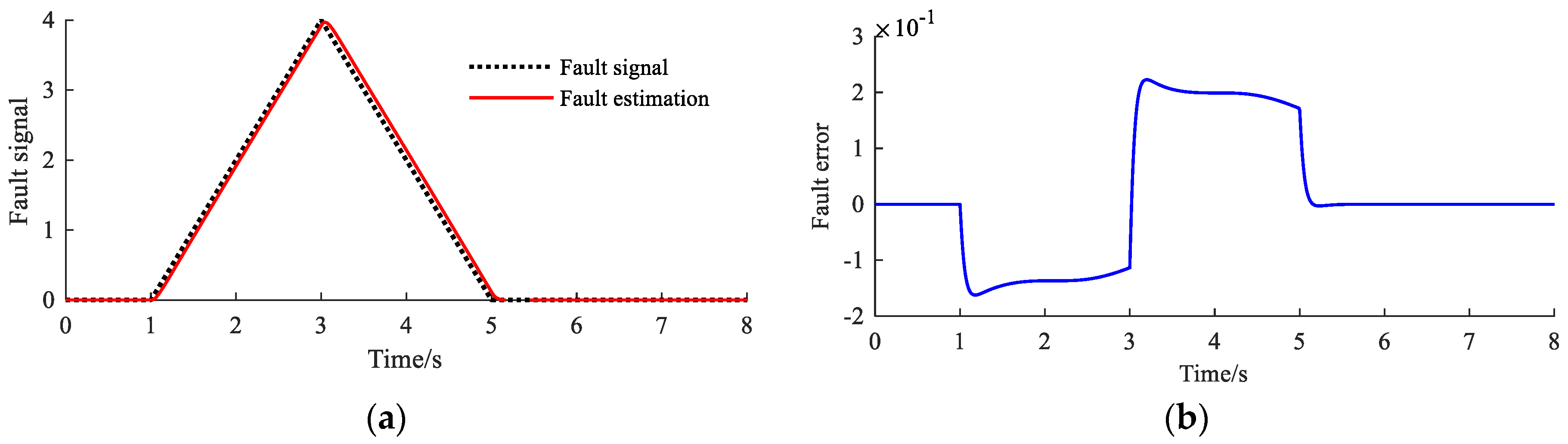
It is assumed that there was an actuator ramp fault at the front and rear suspension, i.e., the system faults occurred at t_f = 1 s with a slope of β_f = 2, and t_f = 3 s with a slope of β_f = −2, successively. Figure 4a shows the time evolution of the fault with its estimate value, whereas Figure 4b reveals the fault error. It was observed that the amplitude of the fault error remained no more than ±0.2. Additionally, the root-mean-square (RMS) values of the fault and fault estimation were 1.4535 and 1.4756, respectively, and the fault estimated error was only 1.52% for the fault signal.

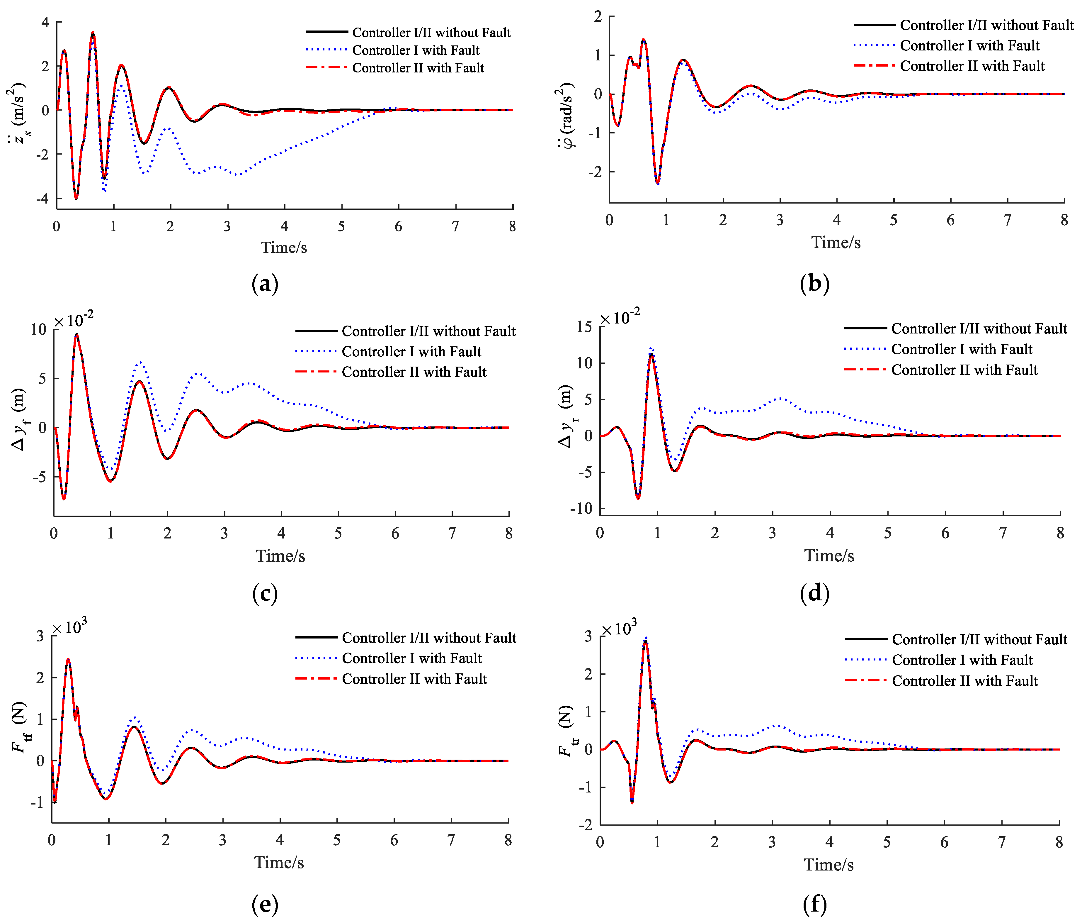
The comparisons of ${\ddot{z}}_s$, $\ddot{\varphi }$, Δy_f, Δy_r, and F_tf, F_tr for an active suspension system with different control schemes in a time-domain are presented in Figure 5, wherein the conventional H_∞ weighted output feedback controller was denoted as Controller I, the proposed active fault-tolerant controller was denoted as Controller II. It is seen from the black solid line in Figure 5 that the performance responses of Controller II and Controller I were almost the same under fault-free condition, which showed that the designed fault compensator controller was only activated when fault occurred. Besides, it can also be obtained from Figure 5 that with the proposed Controller II, the performance indicators of ${\ddot{z}}_s$, $\ddot{\varphi }$, Δy_f, Δy_r, and F_tf, F_tr for the active suspension system could stay stable within a certain range, which demonstrated the robustness of the proposed controller.

By further observing Figure 5a,b, we can arrive at the conclusion that the vertical and pitch angular accelerations of the vehicle body with Controller I could obviously be deteriorated, however, the vertical accelerations of the active suspension system with Controller II could well suppress and eliminate the degradation phenomena caused by the faults, which improved the ride quality of the vehicle suspension system. Moreover, it was clear from Figure 5c,d that the dynamic suspension displacements of the front and rear suspension could be reduced using Controller II, thus preventing suspension breakdown when the suspension deflection was out of range, and further ensuring that vehicle suspension had a better ride comfort and handling stability. Simultaneously, from Figure 5e,f, the tire dynamic loads of the front and rear suspension yielded a smaller variation by using Controller II in the presence of the faults, which improved the tire lifespan and vehicle handling stability.

Figure 6 shows the variation of control force for the designed active fault-tolerant controller. From which, we can obtain the conclusion that the control compensation item will be timely produced to eliminate the performance penalties of the active suspension system brought by the random ramp fault.

4.2. Bump Road Response

A pronounced bump on a smooth road surface was also adopted as the second road disturbance input to further demonstrate the effectiveness of the proposed controller, which is expressed by:

$$x_r(t)=\{\begin{array}{cc}\frac{A_m}{2}(1-\cos \frac{2\pi u}{L}t),\hfill & \hfill 0\le t\le \frac{L}{u}\\ 0,\hfill & \hfill t>\frac{L}{u}\end{array}$$

(26)

where A_m, L and u denote the height and length of bump road, and vehicle forward speed, respectively, and their corresponding values were extracted from literature [27] as A_m = 100 (mm), L = 5 m and u = 45 (km/h).

Meanwhile, in order to verify the effectiveness and applicability of the fault compensation controller, the random fault model of (4) was reconfigured as that, the system faults occurred at t_f = 0.3 s with a slope of β_f = 5, and t_f = 3 s with a slope of β_f = −5, continuously. The fault input signal and its estimation are displayed in Figure 7a, and Figure 7b shows the corresponding fault error with a peak error value of ±0.6. Moreover, the RMS values of the fault and fault estimation were 5.7276 and 5.7829, the fault estimated error was only 0.97% of the fault signal, all of which implied that the designed compensation controller could accurately estimate the fault.

Figure 8 reveals the comparisons of time-domain responses of ${\ddot{z}}_s$, $\ddot{\varphi }$, Δy_f, Δy_r, and F_tf, F_tr for the active suspension system with different control schemes. It was concluded from Figure 7 and Figure 8 that under the fault-free condition, the control performances of the active suspension system with Controller II and Controller I were identical since the fault compensation controller did not work when there was no fault in the system (15). Moreover, it could also be obtained that Controller II could ensure better dynamic responses as opposed to Controller I in the presence of system stochastic faults. Besides, with the Controller II, the performance responses of the active suspension system could reach an asymptotic stability within a short time (about 3 to 5 s), which showed that Controller II had a good robustness to the actuator faults and external disturbances.

Additionally, the variation of control forces for the designed active fault-tolerant controller is shown in Figure 9, and it is seen that the control force will be tuned to compensate for the performance penalties of the active suspension system imposed by the actuator random ramp fault.

It is well known that the RMS value of the acceleration is strictly related to the ride comfort of passengers and it is often used to quantify the amount of the acceleration transmitted to the vehicle body [35]. Additionally, the RMS value of suspension deflection and tire dynamic loads are usually used to verify the performance of the controller [36]. The following equation is used to calculate the RMS value of an n-dimensional vector x as $x_{\mathrm{RMS}}=\frac{\left|\right|x\left|\right|}{\sqrt{n}}=\sqrt{\frac{1}{n}{\displaystyle \sum _{i=1}^n{x}_i^2}}$ $(i=1,2\cdots n)$.

Table 2. Comparisons of root mean square (RMS) values for vehicle suspension performance under bump road.

Index	Controller I/II without Fault	Controller I with Fault	Controller II with Fault
$\ddot{z}$s/(m/s2)	0.8770	1.5053	0.8772
$\ddot{\phi }$/(m2/s3)	0.4141	0.4290	0.4145
Δyf/m	0.0196	0.0277	0.0196
Δyr/m	0.0190	0.0276	0.0191
Ftf/N	411.8726	470.1569	413.0139
Ftr/N	439.6549	486.6650	439.0177

shows the RMS values of $z_{\mathrm{s}}$, $\phi$, Δy_f, Δy_r, and F_tf, F_tr for the active suspension system with the different fault-tolerant control scheme. It was observed that, compared to the dynamic performance indicators of the active suspension system with Controller I and Controller II under the fault-free condition, the RMS values of $z_{\mathrm{s}}$, $\phi$, Δy_f, Δy_r, and F_tf, F_tr for the active suspension system with Controller I under the fault condition had a distinct increase by 71.64%, 3.5%, 40.91%, 40.89%, 14.15%, and 15.02%, respectively. In contrast, the dynamic performance indicators of the active suspension system with Controller II under the same faults were substantially unchanged.

5. Conclusions

In this paper, an observer-based active fault-tolerant controller was proposed for a half-vehicle active suspension system subjected to some generalized stochastic faults. By constructing the augmented fault suspension model, a robust H_∞ weighted output feedback controller was developed to improve the vehicle dynamics performance under a fault-free condition. Then, an H_∞ observer was designed to accurately estimate the fault information with an auxiliary diagnosis system and further to design an H_∞ fault compensation controller to eliminate the effect of the faults on vehicle system performances. Finally, a numerical simulation investigation was provided to verify the effectiveness of the proposed controller under random and bump road surface compared with the classical H_∞ output feedback controller. The results showed that under a fault-free condition, both of the proposed controller and H_∞ output feedback controller could stabilize a vehicle active suspension system with better dynamic performances within a finite time; while under fault condition, compared with the H_∞ output feedback controller, our designed active fault-tolerant controller could accurately estimate the fault information and compensate for the system performance penalties to make the fault suspension system approximate to the performance indicators of the active suspension without faults, which could ensure the reliability of the vehicle active suspension system with the stochastic faults. Future work will focus on the robustness of the control strategy and the experiment for the auxiliary system.

References

- Yildiz, A.S.; Sivrioğlu, S.; Zergeroğlu, E.; Çetin, Ş. Nonlinear adaptive control of semi-active MR damper suspension with uncertainties in model parameters. Nonlinear Dyn. 2014, 79, 2753–2766. [Google Scholar] [CrossRef]
- Savaresi, S.M.; Spelta, C. A single-sensor control strategy for semi-active suspensions. IEEE Trans. Control Syst. Technol. 2009, 17, 143–152. [Google Scholar] [CrossRef]
- Guo, L.; Zhang, L. Robust H∞ control of active vehicle suspension under non-stationary running. J. Sound Vib. 2012, 331, 5824–5837. [Google Scholar] [CrossRef]
- Sun, W.; Pan, H.; Zhang, Y.; Gao, H. Multi-objective control for uncertain nonlinear active suspension systems. IEEE/ASME Trans. Mechatron. 2014, 24, 318–327. [Google Scholar] [CrossRef]
- Wang, H.P.; Mustafa, G.I.; Tian, Y. Model-free fractional-order sliding mode control for an active vehicle suspension system. Adv. Eng. Softw. 2018, 115, 452–461. [Google Scholar] [CrossRef]
- Sun, H.; Li, Y.; Xu, K.; Tong, S. Fuzzy Adaptive Backstepping Control for a Class of Active Suspension Systems. IFAC PapersOnLine 2018, 51, 136–141. [Google Scholar] [CrossRef]
- Yagiz, N.; Hacioglu, Y. Backstepping control of a vehicle with active suspensions. Control Eng. Pract. 2008, 16, 1457–1467. [Google Scholar] [CrossRef]
- Du, H.; Zhang, N. Takagi-Sugeno fuzzy control scheme for electrohydraulic active suspensions. Control Cybern. 2010, 39, 1095–1115. [Google Scholar]
- Li, H.; Yu, J.; Hilton, C.; Liu, H. Adaptive sliding-mode control for nonlinear active suspension vehicle systems using T–S fuzzy approach. IEEE Trans. Ind. Electron. 2013, 60, 3328–3338. [Google Scholar] [CrossRef]
- Bououden, S.; Chadli, M.; Karimi, H.R. A Robust Predictive Control Design for Nonlinear Active Suspension Systems. Asian J. Control 2016, 18, 122–132. [Google Scholar] [CrossRef]
- Bououden, S.; Chadli, M.; Zhang, L.; Yang, T. Constrained model predictive control for time-varying delay systems: Application to an active car suspension. Int. J. Control Autom. 2016, 14, 51–58. [Google Scholar] [CrossRef]
- Urrea, C.; Jamett, M. Sensor and actuator fault analysis in active suspension in view of fault tolerant control. In Proceedings of the Fifth International Conference on Informatics in Control, Automation and Robotics, Intelligent Control Systems and Optimization, Funchal, Madeira, Portugal, 11–15 May 2008; pp. 179–186. [Google Scholar]
- Moradi, M.; Fekih, A. Adaptive PID-sliding-mode fault-tolerant control approach for vehicle suspension systems subject to actuator faults. IEEE Trans. Veh. Technol. 2014, 63, 1041–1054. [Google Scholar] [CrossRef]
- Blanke, M.; Kinnaert, M.; Lunze, J.; Staroswiecki, M. Diagnosis and Fault-Tolerant Control; Springer: Berlin, Germany, 2006. [Google Scholar]
- Jiang, J.; Yu, X. Fault-tolerant control systems: A comparative study between active and passive approaches. Annu. Rev. Control 2012, 36, 60–72. [Google Scholar] [CrossRef]
- Mekki, H.; Boukhetala, D.; Azar, A.T. Sliding modes for fault tolerant control. In Advances and Applications in Sliding Mode Control Systems; Springer: Cham, Switzerland, 2015; pp. 407–433. [Google Scholar]
- Li, H.; Liu, H.; Gao, H.; Shi, P. Reliable fuzzy control for active suspension systems with actuator delay and fault. IEEE Trans. Fuzzy Syst. 2012, 20, 342–357. [Google Scholar] [CrossRef]
- Li, H.; Gao, H.; Liu, H.; Liu, M. Fault-tolerant H∞ control for active suspension vehicle systems with actuator faults. Proc. Inst. Mech. Eng. Inst. J. Syst. Control Eng. 2012, 226, 348–363. [Google Scholar] [CrossRef]
- Sun, W.C.; Pan, H.H.; Yu, J.Y.; Gao, H.J. Reliability control for uncertain half-car active suspension systems with possible actuator faults. IET Control Theory Appl. 2014, 8, 746–754. [Google Scholar] [CrossRef]
- Liu, B.; Saif, M.; Fan, H. Adaptive fault tolerant control of a half-car active suspension systems subject to random actuator failures. IEEE/ASME Trans. Mechatron. 2016, 21, 2847–2857. [Google Scholar] [CrossRef]
- Castaldi, P.; Mimmo, N.; Simani, S. Differential geometry based active fault tolerant control for aircraft. Control Eng. Pract. 2014, 32, 227–235. [Google Scholar] [CrossRef]
- Huang, C.; Naghdy, F.; Du, H. Observer-based fault tolerant controller for uncertain Steer-by-Wire systems using the delta operator. IEEE/ASME Trans. Mechatron. 2018. [Google Scholar] [CrossRef]
- Yin, S.; Wang, G.; Karimi, H.R. Data-driven design of robust fault detection system for wind turbines. Mechatronics 2014, 24, 298–306. [Google Scholar] [CrossRef]
- Lee, T.H.; Lim, C.P.; Nahavandi, S.; Roberts, R.G. Observer-Based H∞ Fault-Tolerant Control for Linear Systems With Sensor and Actuator Faults. IEEE Syst. J. 2018, 2, 1012–1016. [Google Scholar]
- He, X.; Wang, Z.; Qin, L.; Zhou, D. Active fault-tolerant control for an internet-based networked three-tank system. IEEE Trans. Control Syst. Technol. 2016, 24, 2150–2157. [Google Scholar] [CrossRef]
- Kim, H.; Lee, H. Model-based fault-tolerant control for an automotive air suspension control system. Proc. Inst. Mech. Eng. Part D. J. Automob. Eng. 2011, 225, 1462–1480. [Google Scholar] [CrossRef]
- Qiu, J.; Ren, M.; Zhao, Y.; Guo, Y. Active fault-tolerant control for vehicle active suspension systems in finite-frequency domain. IET Control Theory Appl. 2011, 5, 1544–1550. [Google Scholar] [CrossRef]
- Du, H.; Zhang, N. Constrained H∞ control of active suspension for a half-car model with a time delay in control. Proc. Inst. Mech. Eng. Part D J. Automob. Eng. 2008, 222, 665–684. [Google Scholar] [CrossRef]
- Chen, L.; Zhong, M.Q. Parity based fault detection for singular fuzzy systems. Control Decis. 2011, 26, 182–186. [Google Scholar]
- Ping, Z.; Huang, J. Global robust output regulation for a class of multivariable systems. Int. J. Robust Nonlinear 2011, 23, 241–261. [Google Scholar] [CrossRef]
- Chen, Z.; Liu, L.; Huang, J. Global tracking and disturbance rejection of a class of lower triangular systems subject to an unknown exosystem. In Proceedings of the IEEE International Conference on Control and Automation, Christchurch, New Zealand, 9–11 December 2009; pp. 53–58. [Google Scholar]
- Chen, H.; Guo, K.H.; Sun, P.-Y. Constrained H∞ control of active suspensions: An LMI approach. IEEE Trans. Control Syst. Technol. 2005, 13, 412–421. [Google Scholar] [CrossRef]
- Jeung, E.T.; Kim, J.; Hong, P. H∞ output feedback controller design for linear systems with time-varying delayed state. IEEE Trans. Autom. Control 1998, 43, 971–974. [Google Scholar] [CrossRef]
- Pang, H.; Fu, W.Q.; Liu, K. Stability analysis and fuzzy smith compensation control for semi-active suspension systems with time delay. J. Intell. Fuzzy Syst. 2015, 29, 2513–2525. [Google Scholar] [CrossRef] [Green Version]
- Sun, W.; Gao, H.; Kaynak, O. Adaptive backstepping control for active suspension systems with hard constraints. IEEE/ASME Trans. Mechatron. 2013, 18, 1072–1079. [Google Scholar] [CrossRef]
- Pang, H.; Fan, L.; Zeren, X. Variable universe fuzzy control for vehicle semi-active suspension system with MR damper combining fuzzy neural network and particle swarm optimization. Neurocomputing 2018, 306, 130–140. [Google Scholar] [CrossRef]
Figure 1.
Half-vehicle active suspension model.
Figure 2.
The diagram of the active fault tolerant controller.
Figure 3.
The diagram of output feedback H∞ controller for the active suspension system.
Figure 4.
Fault estimation and fault estimation error: (a) Fault estimation, (b) fault error.
Figure 5.
Vehicle performance responses under random road (a) vertical acceleration (b) pitch angular acceleration (c) front suspension deflection (d) rear suspension deflection (e) front tire dynamic load (f) Rear tire dynamic load.
Figure 6.
The control forces of the proposed controller: (a) Front wheel control force and (b) rear wheel control force.
Figure 7.
Fault estimation and fault estimation error: (a) Fault estimation and (b) fault error.
Figure 8.
Vehicle performance responses under random road: (a) Vertical acceleration, (b) pitch angular acceleration, (c) front suspension deflection, (d) rear suspension deflection, (e) front tire dynamic load, (f) rear tire dynamic load.
Figure 9.
The control forces of the proposed controller at (a) the front wheel and (b) the rear wheel.