An Efficient Method to Learn Overcomplete Multi-Scale Dictionaries of ECG Signals

Abstract

The electrocardiogram (ECG) was the first biomedical signal for which digital signal processing techniques were extensively applied. By its own nature, the ECG is typically a sparse signal, composed of regular activations (QRS complexes and other waveforms, such as the P and T waves) and periods of inactivity (corresponding to isoelectric intervals, such as the PQ or ST segments), plus noise and interferences. In this work, we describe an efficient method to construct an overcomplete and multi-scale dictionary for sparse ECG representation using waveforms recorded from real-world patients. Unlike most existing methods (which require multiple alternative iterations of the dictionary learning and sparse representation stages), the proposed approach learns the dictionary first, and then applies a fast sparse inference algorithm to model the signal using the constructed dictionary. As a result, our method is much more efficient from a computational point of view than other existing algorithms, thus becoming amenable to dealing with long recordings from multiple patients. Regarding the dictionary construction, we located first all the QRS complexes in the training database, then we computed a single average waveform per patient, and finally we selected the most representative waveforms (using a correlation-based approach) as the basic atoms that were resampled to construct the multi-scale dictionary. Simulations on real-world records from Physionet’s PTB database show the good performance of the proposed approach.

1. Introduction

Since the development of the first practical apparatus for the recoding of the electrocardiogram (ECG) by Willem Einthoven in 1903, ECGs have been widely used by physicians to diagnose and monitor many cardiac disorders. Indeed, the use of the ECG has become so widespread that it is nowadays routinely used in both clinical and ambulatory settings to obtain a series of indicators related to the health status of patients [1]. This ubiquitous presence of ECGs in the medical field has been greatly enabled by digital signal processing (DSP) techniques: ECGs were the first biomedical signals where DSP algorithms were extensively applied to remove noise and interferences, detect and characterize the different waveforms contained in the ECG, extract the signals of interest (e.g., the fetal ECG) from the composite ECG, etc. [1,2].

By its own nature, the ECG is typically a sparse signal, composed of regular activations (the QRS complexes and other waveforms, such as the P and T waves) and periods of inactivity (corresponding to isoelectric intervals, such as the PQ or ST segments), as well as noise and interferences (baseline wander, powerline interference, electromyographic noise, motion artifacts, etc.) [1]. Since the introduction of the Least Absolute Shrinkage and Selection Operator (LASSO) regularizer by Tibshirani in 1996 [3], many sparse inference and representation techniques have been developed and successfully applied for all kinds of signals [4]: images, sound/audio recordings, biomedical waveforms, etc. However, to obtain a good sparse model for a given signal, it is essential to have an adequate dictionary composed of atoms that properly represent the significant waveforms contained in the observed signals. This has led to the development of many families of dictionaries (based on wavelets and wavelet packets, curvelets, contourlets, etc.) for different applications, as well as several on-line dictionary learning algorithms (e.g., see [5,6,7] for reviews of different dictionary learning methods for sparse inference) that typically require multiple alternative iterations of the dictionary learning and sparse representation stages.

In electrocardiographic signal processing, many approaches have been proposed for the sparse representation of single-channel and multi-channel ECGs using different types of simple analytical waveforms: Gaussians [8,9,10], generalized Gaussians and Gabor dictionaries [11], several families of wavelets (e.g., the Mexican hat or the coiflet4) [12,13], etc. Although these approaches can lead to good practical results, the resulting models usually contain many spurious activations that must be removed to obtain physiologically interpretable signals, for instance by means of a post-processing stage [9,13] or through the minimization of a complex non-convex cost function [14]. Conversely, a customized dictionary, built from real-world signals, will provide a better performance in terms of the reconstruction error obtained for a given level of sparsity. Consequently, several on-line dictionary learning approaches have also been applied, both in the context of sparse inference and compressed sensing (CS), to ECG signals: the K-SVD algorithm in [15], the shift-invariant K-SVD in [16], and the method of optimal directions in [17]. Unfortunately, all these methods have a high computational cost (due to their need to iterate between the dictionary learning and sparse approximation stages) and lead to dictionaries whose atoms do not correspond to real-world signals (thus reducing the interpretability of the sparse model, as well as the ability to easily locate the relevant waveforms). Alternatively, an off-line dictionary construction methodology (where a dictionary with real-world waveforms is initially built and then directly used for CS and sparse modeling without any further modification) was recently proposed by Fira et al. [12,18,19,20]. However, the atoms of the dictionary are either selected randomly from segments of the signal or taken directly from the first half of the ECG without any attempt to determine the most relevant waveforms.

In this work, we describe an efficient method to construct an overcomplete and multi-scale dictionary for sparse ECG representation using waveforms recorded from real-world patients. Unlike on-line dictionary methods (which require multiple alternative iterations of the dictionary learning and sparse representation stages), the proposed approach learns the dictionary first, and then applies a fast sparse inference algorithm, Convolutional Sparse Approximation (CoSA) [21], to model the signal using the constructed dictionary. As a result, our method is much more efficient from a computational point of view than other existing algorithms, thus becoming amenable to deal with long recordings from multiple patients. Regarding the dictionary construction, we locate all the QRS complexes in the training database first, then we compute a single average waveform per patient, and finally we select the most representative waveforms (using a correlation-based approach) as the basic atoms that will be resampled to construct the multi-scale dictionary. With respect to the approach of Fira et al., our method selects the optimal atoms to construct the dictionary, thus resulting in a much more compact solution. Numerical simulations demonstrate that the proposed approach is able to obtain a very sparse representation without missing any QRS complex or introducing spurious activations. Note that a preliminary version of this paper, where a single waveform was used to construct the overcomplete and multi-scale dictionary, was published in [22]. From a theoretical point of view, the main extension with respect to [22] is the proposal of a precise and novel procedure to incorporate multiple waveforms in the construction of the dictionary. Additional improvements, such as the simple and effective approach to remove the edge effects that appear after each resampling stage, have also been introduced in the pre-processing stages. Finally, a much more detailed literature review has been performed and many more numerical simulations, including both patients and channels (leads) not used to derive the dictionary, have been performed to characterize the behavior of the novel scheme.

The rest of the paper is organized as follows. Section 2 formulates the sparse representation problem of ECGs, emphasizing the importance of an appropriate dictionary. Then, in Section 3, we describe in detail the procedure followed to derive a multi-scale dictionary from real-world signals: the database used, the pre-processing steps, and the actual dictionary construction. Finally, Section 4 validates the proposed approach (focusing on the capability of the derived dictionary to model different ECG leads from multiple patients), and the paper is closed by the conclusions and future lines in Section 5. Throughout the paper, we concentrate on the description of the proposed method without focusing on any particular application. However, note that the constructed dictionary can be useful in many practical applications: lossy compression of ECG signals for their storage and transmission [17,20], denoising of ECGs contaminated by different types of interferences using sparse inference techniques [23], compressed sampling and sparse inference for heart rate variability analysis [24], sparse coding for atrial fibrillation (AF) classification [25], etc.

2. Problem Formulation

Let us assume that we have a single discrete-time ECG, $x\left[n\right]$, that has been obtained from a properly filtered and amplified continuous-time ECG, $x_c\left(t\right)$, through uniform sampling with a sampling period $T_s=1/f_s$, i.e., $x\left[n\right]=x_c\left(n{T}_s\right)$. An external ECG captures the electrical activity occurring within the heart that triggers the mechanical cycle (systole and diastole) of the heart. Consequently, it is composed of a set of waveforms that reflect the different stages of the electrical cycle of the heart [1]: atrial depolarization (P waveform), ventricular depolarization (QRS complex) and ventricular repolarization (T waveform). Note that atrial repolarization cannot be observed in external ECGs, since it is masked by the ventricular depolarization, which happens simultaneously and produces a much stronger signal.All of these waveforms repeat themselves regularly during the heart’s electrical cycle (thus leading to the well-known P-QRS-T cycle), although important changes in morphology, as well as fluctuations in amplitude, duration and interarrival times can be observed both for intra-patient and inter-patient recordings. Figure 1 shows an example of a single cycle from a clean synthetic ECG generated using the ECGSYN waveform generator [26] downloaded from Physionet [27], where all the relevant P-QRS-T waveforms, as well as the QRS onset and offset (also known as $\mu$ and j points [28]) can be clearly identified.

On top of the relevant electrical activity, the ECG also contains several types of noise and interference signals [1]: additive white Gaussian noise introduced by the electronic equipment used to acquire the ECGs (sensors, amplifiers and filters), baseline wander caused by the patient’s respiration, powerline interference arising from the electrical network, electromyographic noise, motion artifacts, electrode contact noise, etc. Mathematically, this situation can be modeled as the superposition of the waveforms of interest (QRS complexes, P and T waveforms) as well as all the noise and interferences:

$$x\left[n\right]=\sum _{k=-\infty }^{\infty }{E}_k{\mathsf{\Phi }}_k(t_n-T_k)+ϵ\left[n\right],n=0,\dots ,N-1,$$

(1)

where $T_k$ denotes the arrival time of the kth electrical pulse; $E_k$ its amplitude; ${\mathsf{\Phi }}_k$ is the associated, unknown pulse shape corresponding to QRS complexes, P and T waveforms; and $ϵ\left[n\right]$ the noise and interference term. Note that, in real-world applications, ${\mathsf{\Phi }}_k$, $T_k$, and $E_k$ are not precisely known. However, for the ECG, the typical shapes and durations of the ${\mathsf{\Phi }}_k$ are known for all of the relevant waveforms. Therefore, they can be approximated by a time-shifted, multi-scale dictionary of known waveforms with finite support $M\ll N$ that can then be used to infer the $E_k$ and $T_k$.

More precisely, let us define a set of P candidate waveforms, ${\mathsf{\Gamma }}_p$ for $p=1,\dots ,P$, with a finite support of $M_p$ samples such that $M_1<M_2<\cdots <M_P$ and $M={max}_{p=1,\dots ,P}{M}_p=M_P$. If properly chosen, these waveforms can provide a good approximation of the local behavior of the signal around each sampling point, thus allowing us to approximate Equation (1) through the following model:

$$x\left[n\right]=\sum _{k=0}^{N-M-1}\sum _{p=1}^P{\beta }_{k,p}{\mathsf{\Gamma }}_p[n-k]+\epsilon \left[n\right],n=0,\dots ,N-1,$$

(2)

where the ${\beta }_{k,p}$ are coefficients that indicate the amplitude of the pth waveform shifted to the kth time instant, $t_k=k{T}_s$; and $\epsilon \left[n\right]$ includes also the additional approximation error associated to using Equation (2) instead of Equation (1), as well as all the noise and interferences already contained in $ϵ\left[n\right]$. Let us now group all the candidate waveforms into a single matrix $\mathbf{A}=\left[{\mathbf{A}}_0{\mathbf{A}}_1\cdots {\mathbf{A}}_{N-M-1}\right]$, where the $N\times P$ matrices ${\mathbf{A}}_k$ (for $k=0,\dots ,N-M-1$) have column entries equal to ${\mathsf{\Gamma }}_p[m-k]$ for $m=k,\dots ,k+M-1$ and 0 otherwise. Then, the model of Equation (2) can be expressed more compactly in matrix form as follows:

$$\mathbf{x}=\mathbf{A}\mathit{\beta }+\mathit{\epsilon },$$

(3)

where $\mathbf{x}={[x\left[0\right],\dots ,x[N-1]]}^{\top }$ is an $N\times 1$ vector with all the ECG samples, $\mathit{\beta }={[{\beta }_{0,1},\dots ,{\beta }_{0,P},{\beta }_{1,1},\dots ,{\beta }_{1,P},\dots ,{\beta }_{N-M-1,1},\dots ,{\beta }_{N-M-1,P}]}^{\top }$ is an $(N-M)P\times 1$ coefficients vector, and $\epsilon ={[\epsilon \left[0\right],\dots ,\epsilon [N-1]]}^{\top }$ is the $N\times 1$ noise vector.

Note that the matrix $\mathbf{A}$ can be considered as a global dictionary composed of $N-M$ sub-dictionaries, ${\mathbf{A}}_k$ for $k=0,1,\dots ,N-M-1$, that contain replicas of the candidate waveforms time shifted to $t_0=0$, $t_1=T_s$, …, $t_{N-M-1}=(N-M-1)T_s$. In practice, the usual approach is to either use a single or several different waveforms with different time scales (atoms) to cope with the uncertainty about the shape and duration of the pulses that can be found in $x\left[n\right]$. Hence, as a result, we obtain an overcomplete dictionary (as the number of columns is larger than the number of rows, i.e., $(N-M)P>N$) composed of time-shifted, multi-scale waveforms which resemble the relevant electrical impulses that can be observed in the recorded ECGs. Now, two key questions arise:

• Which is the optimal dictionary to model external ECG signals and how can we construct it?
• Given an overcomplete dictionary, how can we obtain the optimal set of coefficients that represent only the relevant signal components?

Regarding the second question, let us remark that the only unknown term in Equation (3) is $\mathit{\beta }$ when the dictionary is fixed. A classical solution to obtain this set of coefficients $\mathit{\beta }$ is then minimizing the $L_2$ norm of the error between the model and the observed signal, thus obtaining the least squares (LS) solution:

$${\widehat{\mathit{\beta }}}_{LS}={argmin}_{\mathit{\beta }}{\parallel \mathbf{x}-\mathbf{A}\mathit{\beta }\parallel }_2^2,$$

(4)

with ${\parallel ·\parallel }_2$ denoting the $L_2$ norm of a vector. The solution of Equation (4) is not unique, as it requires solving an overdetermined system of linear equations, but the standard solution (i.e., the solution that minimizes the $L_2$ norm of the obtained coefficients) is ${\widehat{\mathit{\beta }}}_{LS}={\mathbf{A}}^{♯}\mathbf{x}$, where ${\mathbf{A}}^{♯}={\left({\mathbf{A}}^{\top }\mathbf{A}\right)}^{-1}{\mathbf{A}}^{\top }$ denotes the pseudoinverse of $\mathbf{A}$. (Note that, even though ${\widehat{\mathit{\beta }}}_{LS}$ can be computed analytically from a theoretical point of view, it requires inverting an $(N-M)P\times (N-M)P$ matrix. Hence, we can easily encounter computational or numerical problems when $(N-M)P$ is large and/or $\mathbf{A}$ is ill-conditioned.) However, the LS approach leads to a solution where all the coefficients in ${\widehat{\mathit{\beta }}}_{LS}$ are likely to be non-zero. This solution does not take into account the sparse nature of the relevant waveforms in $x\left[n\right]$ and results in overfitting, as part of the noise and interference terms are also implicitly modeled by the first term in Equation (3). Hence, a better alternative in this case is explicitly enforcing sparsity in $\mathit{\beta }$ by applying the so-called LASSO approximation [3], which minimizes a cost function composed of the $L_2$ norm of the reconstruction error and the $L_1$ norm of the coefficient vector:

$$\widehat{\mathit{\beta }}={argmin}_{\mathit{\beta }}{\parallel \mathbf{x}-\mathbf{A}\mathit{\beta }\parallel }_2^2+\lambda {\parallel \mathit{\beta }\parallel }_1,$$

(5)

where ${\parallel ·\parallel }_1$ denotes the $L_1$ norm, and $\lambda$ is a parameter defining the trade-off between the sparsity of $\mathit{\beta }$ and the precision of the estimation: the larger is the value of $\lambda$, the sparser is the solution obtained, but also the larger is the mean squared error.

Regarding the first question, it is obvious that a good dictionary, tailored to the shapes of the relevant waveforms in the ECG, will lead to a sparser representation and thus a better temporal localization of those waveforms. In the particular case of ECG modeling, many families of waveforms have been proposed within the related fields of sparse inference and compressed sensing, as discussed in the Introduction. However, there is increasing evidence that the best dictionaries are those constructed using atoms directly extracted from the signals to be modeled [15,17,20]. In the following, we describe a novel approach to construct a single overcomplete and multi-scale dictionary by learning the most representative waveforms from multiple patients. The goal of this paper is then investigating whether the resulting dictionary is able to model the outputs from multiple patients with a single set of representative waveforms.

3. Multi-Scale Dictionary Derivation

In this section, we describe the novel approach for off-line construction of a single overcomplete and multi-scale dictionary using QRS complexes extracted from multiple ECGs recorded from healthy patients. The database used to construct the dictionary is described first in Section 3.1, and the method is described next: the pre-processing stage in Section 3.2 and the dictionary creation stage in Section 3.3. Finally, the obtained dictionary was stored and applied to attain a sparse reconstruction of the desired ECGs (which may be in the database or not) using the LASSO approach, as described in Section 4.

3.1. Database

To construct the dictionary, we used the Physikalisch-Technische Bundesanstalt (PTB) database, compiled by the National Metrology Institute of Germany for research, algorithmic benchmarking and teaching purposes [29]. The ECGs were collected from healthy volunteers and patients with different heart diseases by Prof. Michael Oeff, at the Dep. of Cardiology of Univ. Clinic Benjamin Franklin in Berlin (Germany), and can be freely downloaded from Physionet [27]. (https://www.physionet.org/physiobank/database/ptbdb/). The database contains 549 records from 290 subjects (aged 17–87 years) composed of 15 simultaneously measured signals: the 12 standard leads plus the 3 Frank lead ECGs [1,2]. Each signal lasts approximately 2 min and is digitized using a sampling frequency $f_s=1000$ Hz with a 16 bit resolution. Out of the 268 subjects for which the clinical summary is available, we selected channel 10 (lead V4) of the first recording of the $Q=51$ healthy patients available in order to build the dictionary.

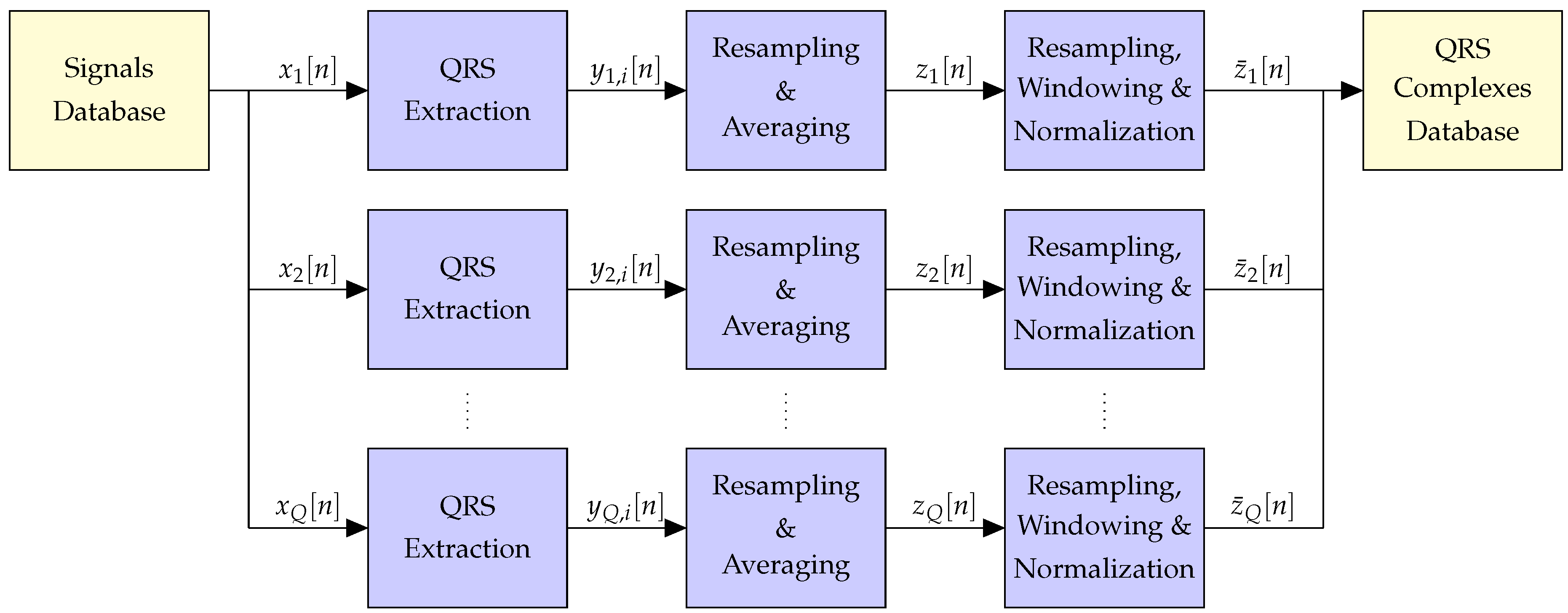
3.2. Pre-Processing

The block diagram of the pre-processing stage is shown in Figure 2. (Let us remark that we focus here on the QRS complexes because they are the most relevant waveforms that can be found in the ECGs. However, the proposed approach can also be applied to construct dictionaries of typical P and T waveforms.) Firstly, all the QRS complexes were extracted separately from each of the Q available ECGs, and those patients for which a significant number of QRS complexes cannot be reliably obtained wree removed from subsequent stages. After resampling to the maximum length of all the QRS complexes found for each of the remaining $Q^{\prime }\le Q$ patients, an individual average QRS complex was obtained per patient. Then, a second resampling stage was applied to the average QRS complexes of all the $Q^{\prime }$ valid patients to ensure that they have the same length, followed by a windowing stage to obtain initial and final samples equal to zero, and a normalization to remove the mean and enforce unit energy on all the signals. Finally, these $Q^{\prime }$ waveforms were stored in a QRS complexes database and used to construct the desired overcomplete dictionary. In the sequel, we provide a detailed description of each of the blocks in Figure 2.

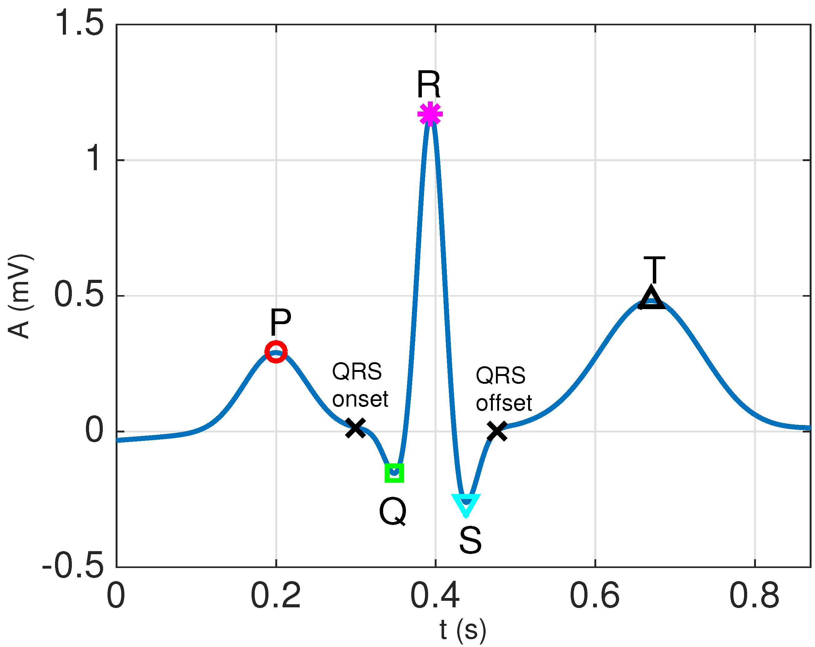
3.2.1. QRS Extraction

The first pre-processing step consists in extracting all the QRS complexes from each of the Q ECGs, $x_q\left[n\right]$ for $q=1,\dots ,Q$. To attain this goal, we followed the approach described in [30]:

• Apply a 4th order Butterworth bandpass filter with cut-off frequencies $f_{c1}=1$ Hz and $f_{c2}=40$ Hz to remove noise and interferences. Forward–backward filtering, with an appropriate choice of the initial state to remove transients [31], is used to avoid phase distortion.
• Locate the positions of the R waveforms using the Pan–Tompkins QRS detector [32].
• Determine the fiducial points that mark the beginning and end of the QRS complexes by tracking backwards and forward from the R peaks, estimating the QRS onset and offset points using the minimum radius of curvature technique, as described in Section 4.2 of [30].

This approach resulted in $Q^{\prime }=44$ valid subjects (i.e., ≈84.6% out of the $Q=51$ available individuals), for which a significant and variable number of QRS complexes ($y_{q,i}\left[n\right]$ for $1\le q\le Q^{\prime }$, $1\le i\le P_q$ and $0\le n\le L_{q,i}-1$), with a variable length of samples for each of them, were extracted for the database used. A total of 6266 QRS complexes were extracted, implying an average of 142.4 QRS complexes per patient (with a maximum of 194 QRS complexes obtained from a single subject) with lengths from 90 to 124 samples (i.e., from 90 to 124 ms).

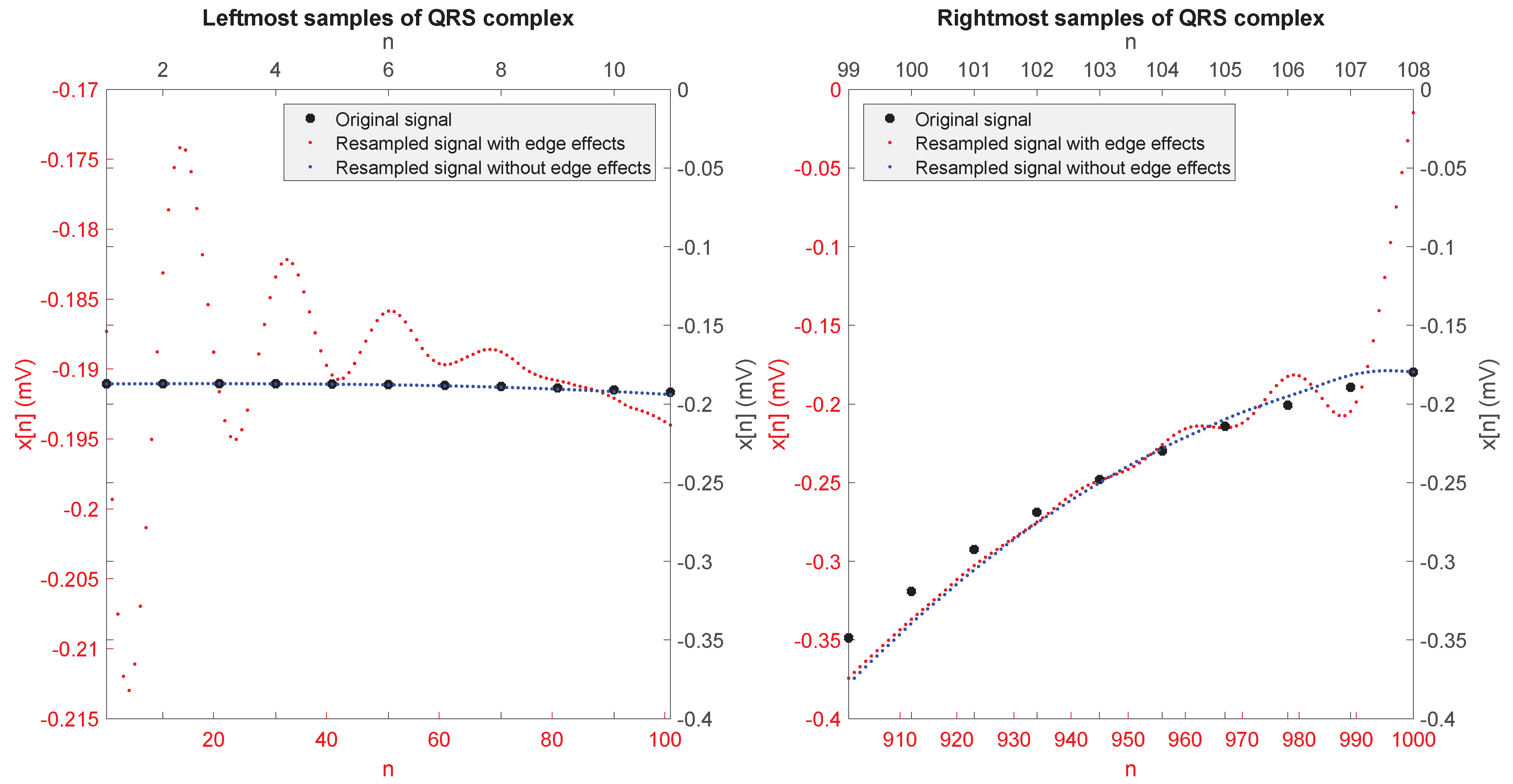
3.2.2. Resampling and Averaging

To compute an average QRS complex for each individual, we need to work with QRS complexes that have a fixed length. (Note that extracting a single waveform per patient can be a limitation. However, since the recordings used in this work correspond to healthy patients and are rather short (less than 2 min), a single waveform is often enough to represent the average QRS complex for each patient. Developing an efficient method to extract multiple waveforms from each patient is a challenging issue that will be considered in future works.) The easiest solution to achieve this goal is resampling the extracted QRS complexes to the maximum length for each patient, $L_{max}^q={max}_{1\le i\le P_q}{L}_{q,i}\le L_{max}={max}_{1\le q\le Q^{\prime }}{L}_{max}^q=124$ samples. A change in the sampling rate of discrete time signals can be accomplished by means of interpolation and decimation [33]. If the ith QRS complex ($i=1,\dots ,P_q$) has a length $L_{q,i}\le L_{max}^q$ samples and $M_{q,i}=\mathrm{GCD}(L_{q,i},L_{max}^q)$, with the Greatest Common Divisor (GCD) being the largest positive integer that divides each of the two integer numbers, then we need first to interpolate by a factor $L_{max}^q/M_{q,i}$ and then to decimate by a factor $L_{q,i}/M_{q,i}$ (i.e., the fractional resampling rate is $L_{max}^q/L_{q,i}\ge 1$).

The aforementioned approach includes a digital lowpass antialiasing filter between the interpolator and the decimator, with a cut-off frequency ${\omega }_c^{q,i}=\pi M_{q,i}/L_{max}^q$ rad, which assumes that the sequence to process starts and ends with sequences of zeroes. Although the recorded ECGs have been initially bandpass filtered to remove baseline wander and other artifacts, the QRS complexes cannot be assumed to start and end with the required zero samples. In fact, the set of available QRS complexes (from the QRS onset to the QRS offset) always contain negative starting and ending values: from −0.0219 to −0.2349 mV for the initial sample, and from −0.0318 to −0.1796 mV for the final sample. As the starting and ending samples of all the QRS complexes are not equal to zero, resampling produces an undesired effect (edge effect), which consists on deviations from the expected values in the starting and ending values of the resampled signals. To remove the edge effect, we propose the following simple and effective approach:

• From the ith QRS complex signal, $y_{q,i}\left[n\right]$ for $n=0,1,\dots ,L_{q,i}-1$, we first constructed the following two sequences:

  $$\begin{array}{cc}\hfill y_{\ell }^{(q,i)}\left[n\right]& =y_{q,i}\left[n\right]-y_{q,i}\left[0\right],\hfill \\ \hfill y_r^{(q,i)}\left[n\right]& =y_{q,i}\left[n\right]-y_{q,i}[L_{q,i}-1],\hfill \end{array}$$

  which are not likely to be affected by the edge effect on their leftmost and rightmost samples, respectively.
• We performed the resampling by the factor $L_{q,i}/L_{max}^i$ separately on $y_{\ell }^{(q,i)}\left[n\right]$ and $y_r^{(q,i)}\left[n\right]$, obtaining two resampled sequences ${\tilde{y}}_{\ell }^{(q,i)}\left[n\right]$ and ${\tilde{y}}_r^{(q,i)}\left[n\right]$.
• The desired resampled sequence is finally given by

  $${\tilde{y}}_{q,i}\left[n\right]=\left\{\begin{array}{cc}{\tilde{y}}_{\ell }^{(q,i)}\left[n\right],\hfill & 0\le n\le ⌊\frac{N}{2}\frac{L_{max}^q}{L_{q,i}}⌋-1;\hfill \\ {\tilde{y}}_r^{(q,i)}\left[n\right],\hfill & ⌊\frac{N}{2}\frac{L_{max}^q}{L_{q,i}}⌋\le n\le ⌊N\frac{L_{max}^q}{L_{q,i}}⌋-1.\hfill \end{array}\right.$$

  (6)

Figure 3 shows the leftmost and rightmost samples corresponding to one of the resampled QRS complexes (from patient 214 in the PTB database) when resampling is performed directly on $y_{q,i}\left[n\right]$. The edge effect on the left and right parts of the signals (i.e., the deviation of the red line with respect to the desired values indicated by the black dots) is evident in this case. On the other hand, when the proposed approach was applied, the resampled sequence (${\tilde{y}}_{q,i}\left[n\right]$) is not affected by the edge effect on either its left or its right side, as also seen in Figure 3.

Finally, the averaged QRS complex for each patient was obtained simply by computing the sample mean for each time instant:

$$z_q\left[n\right]=\frac{1}{P_q}\sum _{i=1}^{P_q}{\tilde{y}}_{q,i}\left[n\right],$$

(7)

with $P_q$ denoting the number of QRS complexes found in the qth ECG.

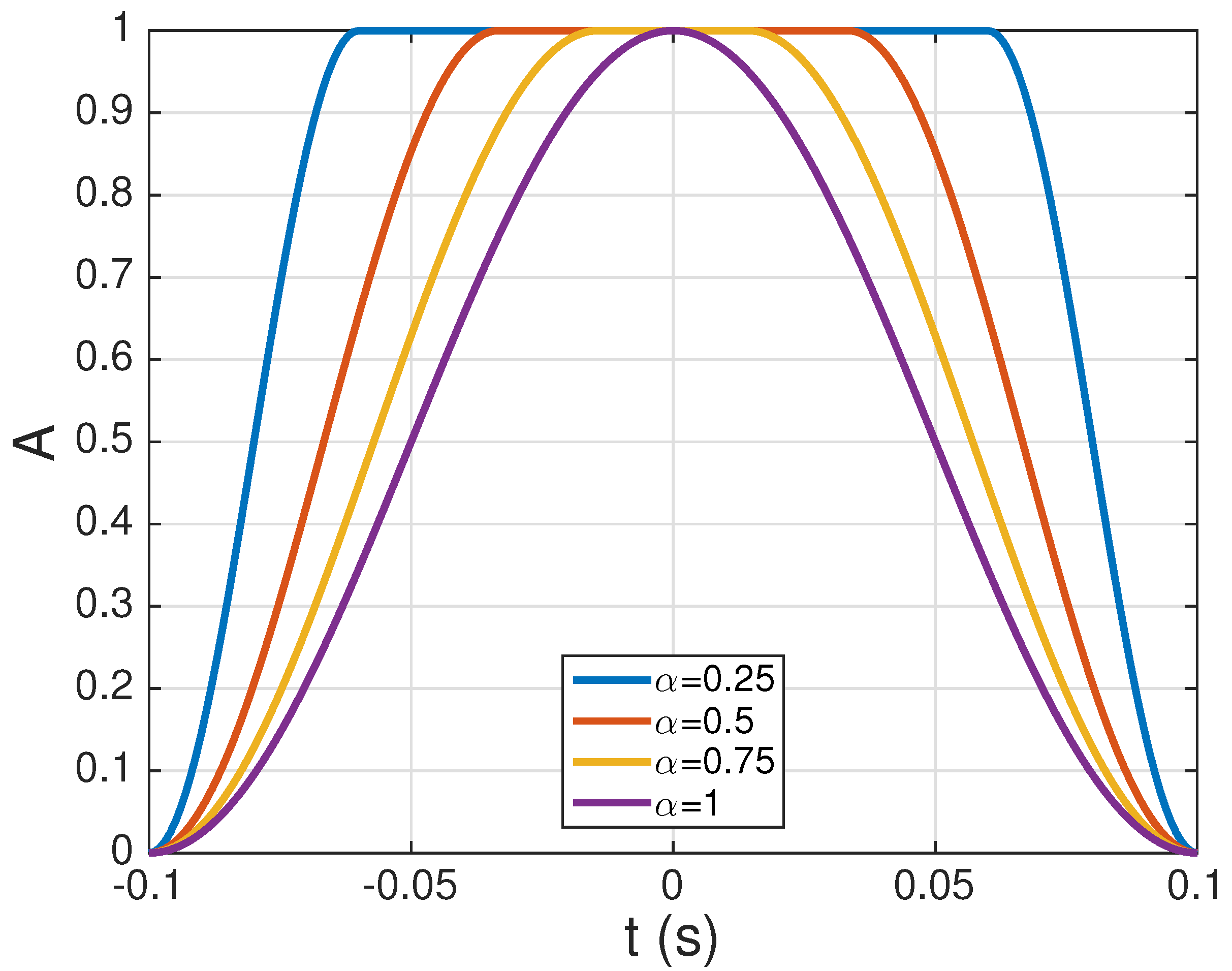
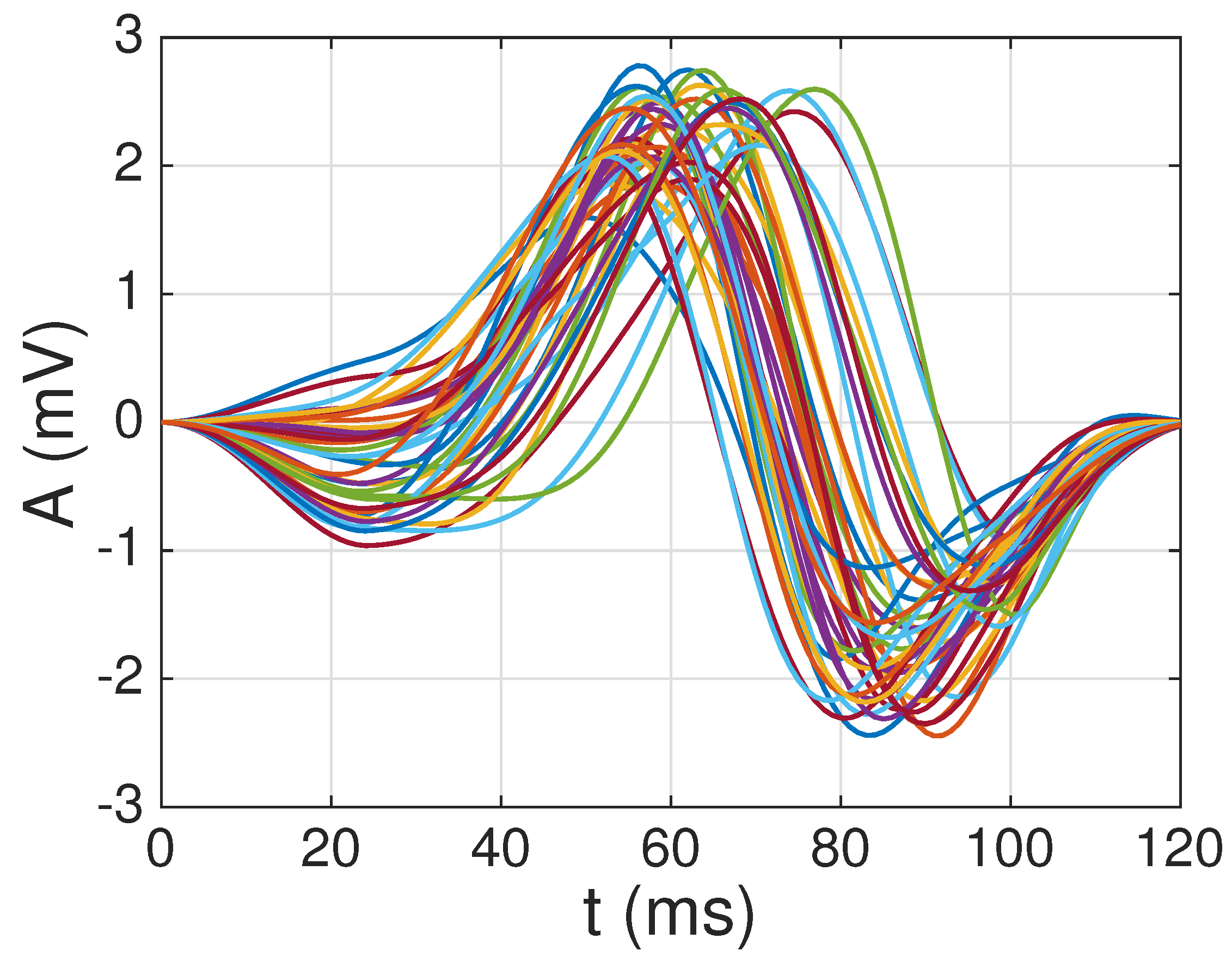
3.2.3. Windowing and Normalization

After averaging, all the averaged QRS complexes were resampled again to obtain $Q^{\prime }$ signals with the same number of samples, $L_{max}={max}_{1\le q\le Q^{\prime }}{L}_{max}^q=124$, using a resampling factor $L_{max}/L_{max}^q$. Then, the resulting signals were windowed to ensure a smooth decay of the QRS complexes towards zero, and normalized by removing their mean and dividing by their standard deviation. The signals that were finally stored in the QRS complex database are

$${\overline{z}}_q\left[n\right]=\frac{{\tilde{z}}_q\left[n\right]w\left[n\right]-{\mu }_q}{{\sigma }_q},$$

(8)

where ${\tilde{z}}_q\left[n\right]$ are the averaged QRS complexes after the second resampling stage (i.e., after ensuring that their sample length is equal to $L_{max}$), ${\mu }_q$ and ${\sigma }_q$ are their sample mean and standard deviations, respectively,

$$\begin{array}{cc}\hfill {\mu }_q& =\frac{1}{L_{max}}\sum _{n=0}^{L_{max}-1}{\tilde{z}}_q\left[n\right]w\left[n\right],\hfill \end{array}$$

(9)

$$\begin{array}{cc}\hfill {\sigma }_q& =\sqrt{\frac{1}{L_{max}-1}\sum _{n=0}^{L_{max}-1}{({\tilde{z}}_q\left[n\right]w\left[n\right]-{\mu }_q)}^2},\hfill \end{array}$$

(10)

and $w\left[n\right]$ is the window used in this case, a window that follows the spectral shape of the raised cosine filter, widely used in digital communications [34], in the time domain: $w\left[n\right]=w_c\left(n{T}_s\right)$ for $n=-(L_{max}-1)/2,\dots ,-1,0,1,\dots ,(L_{max}-1)/2$, with

$$w_c\left(t\right)=\left\{\begin{array}{cc}1,\hfill & \left|t\right|\le (1-\alpha )T_0;\hfill \\ \frac{1}{2}\left[1+cos\left(\frac{\pi }{2\alpha T_0}|t-(1-\alpha )T_0|\right)\right],\hfill & (1-\alpha )T_0<\left|t\right|<(1+\alpha )T_0,\hfill \end{array}\right.$$

(11)

$T_0=\frac{L_{max}-1}{1+\alpha }\frac{T_s}{2}$, and $\alpha$ denoting the roll-off factor that controls the decay of $w_c\left(t\right)$ towards zero: for $\alpha =0$, we have a rectangular window that abruptly goes to zero at $\pm T_0$, whereas for $\alpha =1$ the window is bell-shaped and starts decaying smoothly towards zero immediately after $\left|t\right|>0$. This window, whose time-domain shape is shown in Figure 4 for several values of $\alpha$, ensures that the central samples of the QRS complexes remain undistorted, while their amplitudes quickly decay towards zero at the borders. Throughout the paper, we have always used $\alpha =0.25$.

3.3. Dictionary Construction

After the pre-processing described in the previous section, we have $Q^{\prime }\le Q$ waveforms from different patients stored in the QRS complexes database. These waveforms (${\overline{z}}_q\left[n\right]$ for $1\le q\le Q^{\prime }$ and $0\le n\le L_{max}-1$) could be directly used to build the sub-dictionaries. However, they are highly correlated and thus the resulting dictionary would provide a poor performance and lead to a high computation time. Therefore, to obtain a reduced dictionary composed of distinct shapes, we performed the procedure described in the following sections.

3.3.1. Selection of the First Atom

For the first atom of the dictionary, we sought the most representative waveform in the QRS complexes database. Indeed, if we intend to construct a sparse model for all the ECGs of all the patients using a single basis signal, then we should choose a waveform which resembles as closely as possible the set of QRS complexes (the most relevant part of the ECGs) in the different patients. To achieve this goal, using the average signals stored in the QRS complexes database, we followed two steps:

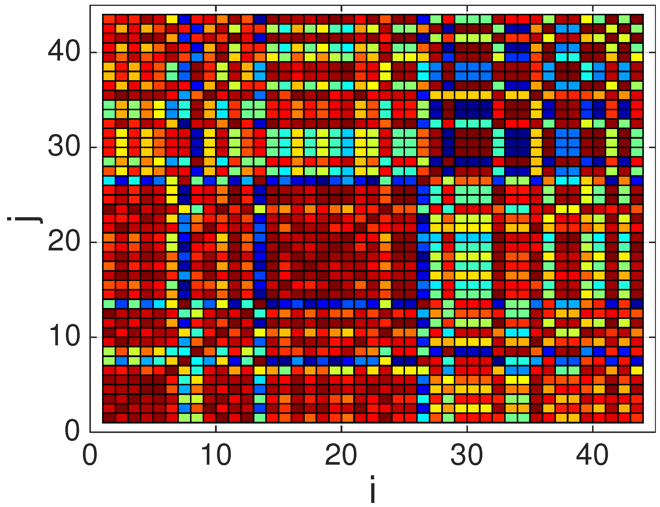
• Compute a $Q^{\prime }\times Q^{\prime }$ correlation matrix $\mathbf{C}$, whose ${\left(Q^{\prime }\right)}^2$ elements correspond to Pearson’s correlation coefficient among each pair of waveforms in the QRS complexes database (in practice, only $Q^{\prime }(Q^{\prime }-1)/2$ coefficients have to be computed, since ${\rho }_{ii}=1$ and ${\rho }_{ij}={\rho }_{ji}$$\forall i,j\in \{1,\dots ,Q^{\prime }\}$).

  $${\rho }_{ij}=\frac{C_{ij}}{\sqrt{C_{ii}{C}_{jj}}}=C_{ij},$$

  (12)

  where $C_{ij}$ denotes the cross-covariance between the ith and jth waveforms at lag 0 (i.e., without any time shift), and the last expression (${\rho }_{ij}=C_{ij}$) is due to the energy normalization described in Section 3.2.3, which implies that $C_{ii}=0\forall i$.
• Select the waveform with the highest average correlation (in absolute value) with respect to all the other candidate waveforms, i.e.,

  $${\ell }_0={argmax}_{i=1,\dots ,Q^{\prime }}\sum _{j=1}^{Q^{\prime }}|{\rho }_{ij}|,$$

  (13)

  which corresponds to the most representative waveform of all the candidate waveforms.

3.3.2. Selection of Additional Atoms

Additional atoms can be incorporated to the dictionary in order to increase its flexibility in representing different ECGs. These atoms should be constructed using highly correlated waveforms with respect to the remaining candidates (to obtain representative dictionary atoms), as well as with low absolute correlation with respect to already selected waveforms (to avoid similar atoms). Here, we propose to use the following procedure to select a total of K representative waveforms:

• Set the number of accepted atoms equal to one ($k=1$), the pool of candidate waveforms as $\mathcal{C}=\{1,\dots ,{\ell }_0-1,{\ell }_0+1,\dots ,Q^{\prime }\}$ (i.e., all the waveforms except for the one selected for the first atom), the pool of accepted waveforms as $\mathcal{A}=\left\{{\ell }_0\right\}$, and construct a reduced correlation matrix by removing the row and column corresponding to the first atom selected from the global correlation matrix $\mathbf{C}$:

  $${\mathbf{C}}_r=\left[\begin{array}{cc}{\mathbf{C}}_{1:{\ell }_0-1,1:{\ell }_0-1}& {\mathbf{C}}_{1:{\ell }_0-1,{\ell }_0+1:Q^{\prime }}\\ {\mathbf{C}}_{{\ell }_0+1:Q^{\prime },1:{\ell }_0-1}& {\mathbf{C}}_{{\ell }_0+1:Q^{\prime },{\ell }_0+1:Q^{\prime }}\end{array}\right].$$

  (14)
• WHILE$k<K$:

  (a)

  Select, from the remaining waveforms in the pool of candidates, the one with the highest average correlation (in absolute value) with respect to all the other candidate waveforms in the pool, i.e.,

  $${\tilde{\ell }}_k={argmax}_{i=1,\dots ,Q^{\prime }-k}\sum _{j=1}^{Q^{\prime }-k}|{\mathbf{C}}_r(i,j)|,$$

  (15)

  and obtain the associated index, ${\ell }_k$, in the original set of candidate waveforms.

  (b)

  Compute the maximum correlation (in absolute value) between the selected candidate and all the already accepted atoms,

  $${\rho }_{max}=\underset{i=0,\dots ,k-1}{max}\left|\mathbf{C}({\ell }_k,{\ell }_i)\right|.$$

  (16)

  (c)

  Remove the ${\ell }_k$th waveform from the pool of candidates (i.e., set $\mathcal{C}=\mathcal{C}\backslash \left\{{\ell }_k\right\}$), and construct a new reduced matrix (${\mathbf{C}}_r$) by removing the ${\tilde{\ell }}_k$th row and column from the current ${\mathbf{C}}_r$.

  (d)

  IF${\rho }_{max}<\gamma$ (with $0\le \gamma \le 1$ denoting a pre-defined maximum correlation threshold), THEN add the selected waveform to the pool of accepted atoms (i.e., $\mathcal{A}=\mathcal{A}\cup \left\{{\ell }_k\right\}$), and set $k=k+1$.

  END

Note that the value of $\gamma$ sets an upper bound on the number of waveforms that can be accepted for a given set of candidate waveforms. Therefore, K is the maximum number of waveforms that can be accepted in the previous algorithm, but the number of waveforms selected can actually be smaller than K. See Section 4.1 for a detailed description of the values of $\gamma$ and K used in this work.

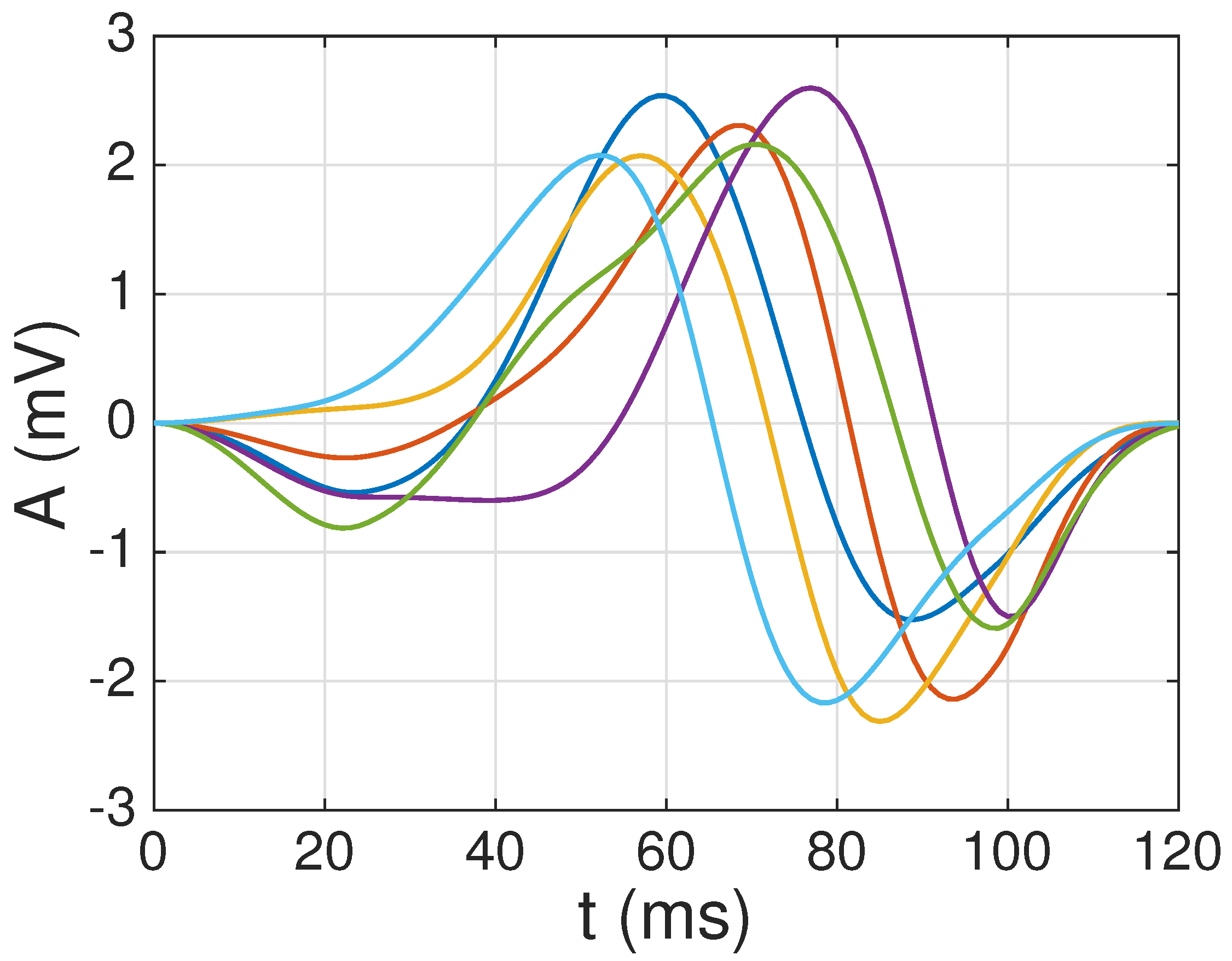
3.3.3. Construction of the Multi-Scale Dictionary

Finally, the K selected waveforms were resampled to obtain an overcomplete and multi-scale sub-dictionary composed of R different time scales. Note that the total number of atoms is thus $P=KR$, corresponding to K different waveforms with R distinct time scales for each one. In this case, we used $R=11$ different time scales spanning a time frame slightly wider than the typical durations of QRS complexes: $60,70,\dots ,160$ ms. Note also that the global dictionary is simply obtained by performing $N-M$ different time shifts of the resulting sub-dictionary [13].

4. Numerical Results

In this section, we first detail the construction of the dictionary and then present the application of the resulting dictionary to perform the sparse reconstruction of the signals from different patients.

4.1. Dictionary Construction

As mentioned earlier, to construct the dictionary, we used channel 10 (lead V4) from the first register of the $Q=51$ healthy patients in the PTB database: Patients 104, 105, 116, 117, 121, 122, 131, 150, 155, 156, 166, 169, 170, 172–174, 180, 182, 184, 185, 198, 214, 229, 233–248, 251, 252, 255, 260, 263, 264, 266, 267, 276, 277, 279, and 284. From this whole set of patients, we were able to obtain reliable average QRS complexes for $Q^{\prime }=44$ Patients: 104, 105, 117, 121, 122, 131, 150, 155, 156, 169, 170, 174, 180, 182, 184, 185, 198, 214, 229, 234–248, 251, 252, 260, 263, 264, 267, 276, 277, 279, and 284. The remaining $Q-Q^{\prime }=7$ patients (116, 166, 172, 173, 233, 255, and 266), where the extraction of the QRS complexes fails, were used as the test set. The average waveforms for the $Q^{\prime }=44$ patients, after resampling to $L=124$ samples (i.e., 124 ms), windowing and normalization, can be seen in Figure 5. Note that, as expected, there is a large degree of similarity among all the waveforms, since they all correspond to regular heartbeats from healthy patients. This similarity is illustrated also by the color plot of the absolute value of the correlation coefficient in Figure 6. Note the large correlation (corresponding to dark red points) among most waveforms. For this reason, in [22], we decided to extract a single waveform in order to construct the multi-scale and overcomplete dictionary. However, in Figure 6, we also notice that some waveforms exhibit low correlation values (as shown by blue points). This motivates us to explore here the performance as more than one waveform is extracted from the pool of average QRS complexes shown in Figure 5 in order to construct the dictionary.

To build dictionaries composed of different waveforms, we tested several threshold levels: $\gamma =0.1,0.2,\dots ,0.9$. Note that the larger is the value of $\gamma$ the less restrictive is the condition to incorporate a new atom to the dictionary, and thus the larger is the number of final atoms (K) used: for $\gamma =0$, we would always obtain $K=1$ atoms (since no new atoms can be incorporated after the first one), whereas, for $\gamma =1$, we would obtain $K=Q^{\prime }$ (as all waveforms would be considered valid). Following this approach, we obtained $K=1$ atoms for $\gamma \le 0.2$, $K=2$ atoms for $0.3\le \gamma \le 0.6$, $K=3$ atoms when $\gamma =0.7$, $K=4$ atoms when $\gamma =0.8$, and $K=6$ atoms when $\gamma =0.9$. Figure 7 shows the six atoms selected for $\gamma =0.9$. Note that, since we followed a deterministic procedure, the first atom was the one obtained for $K=1$ (i.e., when $\gamma \le 0.2$), the first and second ones were those obtained for $K=2$ (i.e., for $0.3\le \gamma \le 0.6$), and so on.

Finally, the selected waveforms for $K=1,\dots ,6$ were resampled in such a way that their duration ranged from 60 ms to 160 ms (with a time step of 10 ms). The resulting base dictionary, composed of $P=11\times K=11,22,\dots ,66$ atoms, is shown in Figure 8 for $K=6$. The final multi-scale and overcomplete dictionary consists of these P waveforms time shifted to the $N-M$ locations of the sampled ECGs, implying that its size is $N\times P(N-M)$. For instance, for $N=115,200$ samples (a typical signal size in the PTB database) and $M=160$ samples (the maximum support of the selected waveforms), the size of the matrix dictionary ranges from $N\times 11(N-M)=115,200\times 1,265,440$ for $K=1$ up to $N\times 66(N-M)=115,200\times 7,592,640$ for $K=6$.

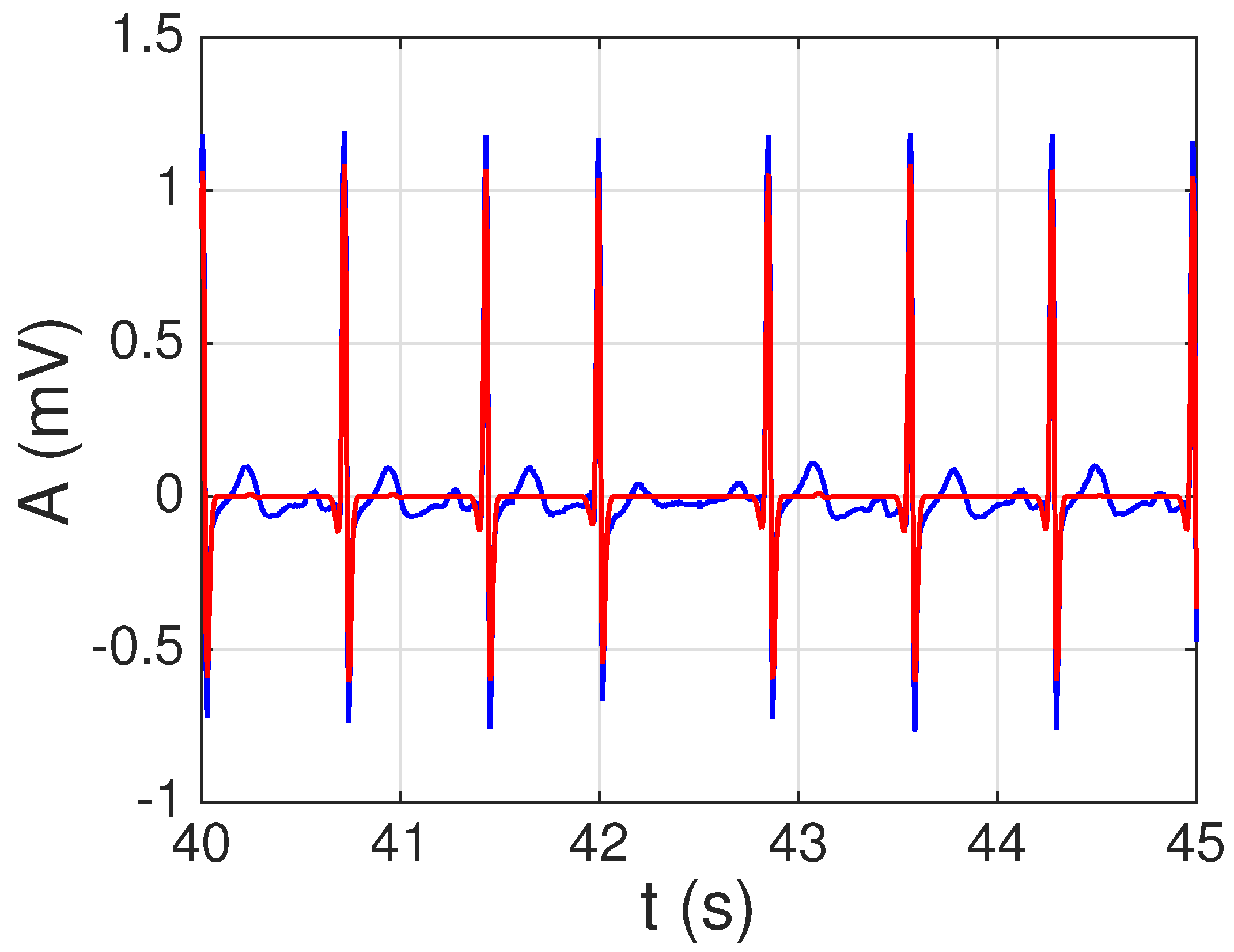
4.2. Sparse ECG Representation

We next tested the constructed dictionary on 21 recordings corresponding to 17 healthy patients from the PTB database. Our main goal was determining whether the constructed dictionary (which is not patient-specific) can be effectively used to perform a sparse representation of ECG signals from multiple patients. To solve Equation (5), we used the CoSA algorithm recently proposed in [21], which allows us to process the $N\approx$ 115,200 samples (almost 2 min of recorded time) of the whole signal at once (i.e., without having to partition it into several segments that have to be processed separately) in a reasonable amount of time. Since several signals showed a significant degree of baseline wander, before applying CoSA all signals were filtered using a third-order high-pass IIR (infinite impulse response) Butterworth filter designed using Matlab’s filterDesigner tool: stop-band frequency $f_{stop}=0.1$ Hz; pass-band frequency $f_{pass}=1$ Hz; minimum stop-band attenuation $A_{stop}=40$ dB; and maximun pass-band attenuation $A_{pass}=1$ dB. Forward–backward filtering was applied again to avoid phase distortion. An example of the reconstructed signal using $K=1$ and $\lambda =20$ is shown in Figure 9. Note that all the QRS complexes (our main goal here) are properly represented by the sparse model. By increasing the number of signals (K), and especially by decreasing the sparsity factor ($\lambda$), a better model that also includes the P and T waveforms can be obtained. However, let us remark that this is not our main goal. Indeed, a better option to model the P and T waveforms would be constructing specific dictionaries of P and T waveforms: either using synthetic waveforms (e.g., Gaussians) or applying the proposed approach to construct real-world dictionaries of P and T waveforms. We intend to explore this issue in future works, constructing mega-dictionaries of P-QRS-T waveforms which are able to model all the relevant activations in the ECGs.

To measure the effectiveness of the proposed approach, we used several performance metrics that measure both the model’s sparsity and its accuracy in representing the original signal. On the one hand, the sparsity was gauged by the coefficient sparsity (C-Sp),

$$\mathrm{C-Sp}(\%)=\frac{{\parallel \mathit{\beta }\parallel }_0}{(N-M)P}\times 100$$

(17)

which measures how many non-null coefficients (out of the total ones) are required to represent the signal, and the signal sparsity (S-Sp),

$$\mathrm{S-Sp}(\%)=\frac{{\parallel \mathbf{x}\parallel }_0}{N}\times 100$$

(18)

which measures how many samples of the signal’s approximation (out of the total number of samples) are not equal to zero. Note that ${\parallel ·\parallel }_0$ indicates the $L_0$ “norm” of a vector, i.e., its number of non-null elements. On the other hand, the reconstruction error was measured by the normalized mean squared error (NMSE) and its logarithmic counterpart, the reconstruction signal to noise ratio (R-SNR):

$$\begin{array}{cc}\hfill \mathrm{NMSE}(\%)& =\frac{{\parallel \mathbf{x}-\mathbf{A}\mathit{\beta }\parallel }_2^2}{{\parallel \mathbf{x}\parallel }_2^2}\times 100\hfill \end{array}$$

(19)

$$\begin{array}{cc}\hfill \mathrm{R-SNR}\left(\mathrm{dB}\right)& =10·{log}_{10}\left(\mathrm{NMSE}\right),\hfill \end{array}$$

(20)

where ${\parallel ·\parallel }_2^2$ denotes the squared $L_2$ norm of a vector.

The results, for the four performance measured previously described, are displayed in Figure 10. On the left hand side, we show the results (mean value and standard deviation) for the first 10 patients in the training set: Patients 104, 105, 117, 121, 122, 131, 150, 155, 156, and 169. On the right hand side, we show the results (mean value and standard deviation again) for the 11 signals in the test set: Patients 116, 166, 172, 173, 233 (5 recordings), 255, and 266. Note the large sparsity attained in all cases (especially as $\lambda$ increases), and the good reconstruction error for small/moderate values of $\lambda$ (i.e., $\lambda \le 5$). Note also the improvement in performance when incorporating additional waveforms to the dictionary (e.g., for $\lambda =2$ there is a 3.32 dB improvement in mean R-SNR for the patients in the test set when using $K=6$ instead of $K=1$), although this comes at the expense of a reduction in the signal sparsity (e.g., for the same case, the mean S-Sp goes down by 4.2% when using $K=6$ instead of $K=1$). Finally, let us remark that there are no substantial differences between the performance on signals from the test set (i.e., signals used to build the dictionary) and signals from the training set (i.e., signals not used to build the dictionary), as evidenced by the similarity of curves on the left hand side and right hand side of Figure 10.

As a last performance check, we applied the Pan–Tompkins algorithm to the reconstructed signal in order to test whether the sparse model introduced some distortion in the location of the QRS complexes. As a result, we found that all the QRS complexes were always properly detected and located within two samples (i.e., $\pm 2$ ms) of the QRS complexes found in the original signal, even in the sparsest case (i.e., with $K=1$ and $\lambda =20$). Therefore, if we are only interested in the QRS complexes or some analysis derived from them (e.g., heart rate variability studies), the proposed model is a very good option to construct a sparse model that keeps all the relevant information.

4.3. Sparse ECG Representation of Other Channels

In this section, we investigate the feasibility of using the dictionary learnt on lead V4 to represent ECGs recorded in other leads. To do so, we used the constructed dictionary to model all 15 channels (leads) available for Patient 104. Let us emphasize that no signals at all from any of the other 14 leads available were used to derive the dictionary, since all samples used from all the patients during the dictionary construction stage correspond to lead V4.

Table 1. Performance of the constructed dictionary (using waveforms extracted from lead V4) on other leads from Patient 104 not used to construct the dictionary.

Channel	Lead	C-Sp (%)	S-Sp (%)	NMSE (%)	R-SNR (dB)
1	I	86.5245	11.0095	4.1476	13.8220
2	II	83.6901	5.1302	1.8310	17.3732
3	III	92.0191	38.1580	5.1706	12.8646
4	aVR	85.4093	6.0408	2.5404	15.9510
5	aVL	92.9162	61.9314	10.2057	9.9116
6	aVF	88.1383	12.0894	3.0323	15.1823
7	V1	87.4629	5.5182	3.1652	14.9960
8	V2	90.7240	51.0356	3.0689	15.1302
9	V3	86.5196	40.1319	2.3935	16.2097
10	V4	83.1699	26.8689	2.9814	15.2557
11	V5	80.9004	5.1181	2.1296	16.7170
12	V6	81.0859	3.4931	1.6270	17.8862
13	Vx	80.1663	4.3333	1.7768	17.5037
14	Vy	93.0671	62.7804	11.4420	9.4150
15	Vz	94.0583	69.9991	5.8457	12.3316

displays the results for $\lambda =1$ and $K=2$, showing that good results are obtained in general for most of the leads. Indeed, the performance for several leads (II, aVR, V5, V6 and Vx) in terms R-SNR is better than for lead v4, which was used to construct the dictionary, and poor R-SNR results were only attained for leads aVL and Vy. Similar conclusions were obtained when considering other values of $\lambda$ and K. Overall, this shows the feasibility of constructing a single multi-scale and overcomplete dictionary (possibly using QRS complexes extracted from several leads) for multiple channels.

5. Conclusions

In this paper, we have described a novel mechanism to derive a realistic, multi-scale and overcomplete dictionary from recorded real-world ECG signals. The dictionary was constructed offline, thus avoiding the computational burden of on-line approaches and ensuring the scalability of the proposed methodology for large datasets with many individuals and/or sample sizes. The obtained dictionary was been used to perform an accurate sparse representation of several ECGs recorded from healthy patients, showing that it can properly capture all the QRS complexes without introducing false alarms. Potential future lines include testing the proposed approach on a larger number of patients (especially including subjects with cardiac pathologies), the construction of dictionaries composed of multiple waveforms (e.g., P and T waveforms), and the combination of waveforms extracted from real patients with synthetic waveforms.

References

- Sörnmo, L.; Laguna, P. Bioelectrical Signal Processing in Cardiac and Neurological Applications; Academic Press: Cambridge, MA, USA, 2005. [Google Scholar]
- Clifford, G.; Azuaje, F.; McSharry, P. (Eds.) Advanced Methods and Tools for ECG Data Analysis; Artech House: Norwood, MA, USA, 2009. [Google Scholar]
- Tibshirani, R. Regression shrinkage and selection via the Lasso. J. R. Stat. Soc. Ser. B (Methodol.) 1996, 58, 267–288. [Google Scholar] [CrossRef]
- Elad, M. Sparse and Redundant Representations: From Theory to Applications in Signal and Image Processing; Springer: Berlin, Germany, 2010. [Google Scholar]
- Kreutz-Delgado, K.; Murray, J.F.; Rao, B.D.; Engan, K.; Lee, T.W.; Sejnowski, T.J. Dictionary learning algorithms for sparse representation. Neural Comput. 2003, 15, 349–396. [Google Scholar] [CrossRef] [PubMed]
- Rubinstein, R.; Bruckstein, A.M.; Elad, M. Dictionaries for sparse representation modeling. Proc. IEEE 2010, 98, 1045–1057. [Google Scholar] [CrossRef]
- Tosic, I.; Frossard, P. Dictionary learning. IEEE Signal Process. Mag. 2011, 28, 27–38. [Google Scholar] [CrossRef]
- Billah, M.; Mahmud, T.; Snigdha, F.; Arafat, M. A novel method to model ECG beats using Gaussian functions. In Proceedings of the 2011 4th International Conference on Biomedical Engineering and Informatics (BMEI), Shanghai, China, 15–17 October 2011; Volume 2, pp. 612–616. [Google Scholar]
- Monzón, S.; Trigano, T.; Luengo, D.; Artés-Rodríguez, A. Sparse spectral analysis of atrial fibrillation electrograms. In Proceedings of the 2012 IEEE International Workshop on Machine Learning for Signal Processing, Santander, Spain, 23–26 September 2012; pp. 1–6. [Google Scholar]
- Trigano, T.; Kolesnikov, V.; Luengo, D.; Artés-Rodríguez, A. Grouped sparsity algorithm for multichannel intracardiac ECG synchronization. In Proceedings of the 2014 22nd European Signal Processing Conference (EUSIPCO), Lisbon, Portugal, 1–5 September 2014; pp. 1537–1541. [Google Scholar]
- Divorra-Escoda, O.; Granai, L.; Lemay, M.; Hernandez, J.M.; Vandergheynst, P.; Vesin, J.M. Ventricular and atrial activity estimation through sparse ECG signal decompositions. In Proceedings of the 2006 IEEE International Conference on Acoustics Speech and Signal Processing Proceedings, Toulouse, France, 14–19 May 2006; Volume II, pp. 1060–1063. [Google Scholar]
- Fira, M.; Goras, L.; Barabasa, C.; Cleju, N. On ECG compressed sensing using specific overcomplete dictionaries. Adv. Electr. Comput. Eng. 2010, 10, 23–28. [Google Scholar] [CrossRef]
- Luengo, D.; Monzón, S.; Trigano, T.; Vía, J.; Artés-Rodríguez, A. Blind analysis of atrial fibrillation electrograms: A sparsity-aware formulation. Integr. Comput.-Aided Eng. 2015, 22, 71–85. [Google Scholar] [CrossRef]
- Luengo, D.; Vía, J.; Monzón, S.; Trigano, T.; Artés-Rodríguez, A. Cross-products LASSO. In Proceedings of the 2013 IEEE International Conference on Acoustics, Speech and Signal Processing, Vancouver, BC, Canada, 26–31 May 2013; pp. 6118–6122. [Google Scholar]
- Wang, C.; Liu, J.; Sun, J. Compression algorithm for electrocardiograms based on sparse decomposition. Front. Electr. Electron. Eng. China 2009, 4, 10–14. [Google Scholar] [CrossRef]
- Mailhé, B.; Gribonval, R.; Bimbot, F.; Lemay, M.; Vandergheynst, P.; Vesin, J.M. Dictionary learning for the sparse modelling of atrial fibrillation in ECG signals. In Proceedings of the 2009 IEEE International Conference on Acoustics, Speech and Signal Processing, Taipei, Taiwan, 19–24 April 2009; pp. 465–468. [Google Scholar]
- Polania, L.F.; Barner, K.E. Multi-scale dictionary learning for compressive sensing ECG. In Proceedings of the IEEE Digital Signal Processing and Signal Processing Education Meeting (DSP/SPE), Napa, CA, USA, 11–14 August 2013; pp. 36–41. [Google Scholar]
- Fira, M.; Goras, L.; Barabasa, C.; Cleju, N. ECG compressed sensing based on classification in compressed space and specified dictionaries. In Proceedings of the 19th European Signal Processing Conference (EUSIPCO), Barcelona, Spain, 29 August–2 September 2011; pp. 1573–1577. [Google Scholar]
- Fira, M.; Goras, L.; Barabasa, C. Reconstruction of compressed sensed ECG signals using patient specific dictionaries. In Proceedings of the International Symposium on Signals, Circuits and Systems ISSCS2013, Iasi, Romania, 11–12 July 2013; pp. 1–4. [Google Scholar]
- Fira, M.; Goras, L. On projection matrices and dictionaries in ECG compressive sensing— A comparative study. In Proceedings of the 12th Symposium on Neural Network Applications in Electrical Engineering (NEUREL), Belgrade, Serbia, 25–27 November 2014; pp. 3–8. [Google Scholar]
- Trigano, T.; Shevtsov, I.; Luengo, D. CoSA: An accelerated ISTA algorithm for dictionaries based on translated waveforms. Signal Process. 2017, 139, 131–135. [Google Scholar] [CrossRef]
- Luengo, D.; Meltzer, D.; Trigano, T. Sparse ECG Representation with a Multi-Scale Dictionary Derived from Real-World Signals. In Proceedings of the 41st International Conference on Telecommunications and Signal Processing (TSP), Athens, Greece, 4–6 July 2018; pp. 1–5. [Google Scholar]
- Satija, U.; Ramkumar, B.; Manikandan, M.S. Noise-aware dictionary-learning-based sparse representation framework for detection and removal of single and combined noises from ECG signal. Healthc. Technol. Lett. 2017, 4, 2–12. [Google Scholar] [CrossRef] [PubMed]
- Faust, O.; Acharya, U.R.; Ma, J.; Min, L.C.; Tamura, T. Compressed sampling for heart rate monitoring. Comput. Methods Prog. Biomed. 2012, 108, 1191–1198. [Google Scholar] [CrossRef] [PubMed]
- Whitaker, B.M.; Rizwan, M.; Aydemir, V.B.; Rehg, J.M.; Anderson, D.V. AF classification from ECG recording using feature ensemble and sparse coding. Computing 2017, 44, 1. [Google Scholar]
- McSharry, P.E.; Clifford, G.D.; Tarassenko, L.; Smith, L.A. A dynamical model for generating synthetic electrocardiogram signals. IEEE Trans. Biomed. Eng. 2003, 50, 289–294. [Google Scholar] [CrossRef] [PubMed]
- Goldberger, A.; Amaral, L.A.; Glass, L.; Hausdorff, J.M.; Ivanov, P.C.; Mark, R.G.; Mietus, J.E.; Moody, G.B.; Peng, C.K.; Stanley, H.E. Physiobank, physiotoolkit, and physionet. Circulation 2000, 101, e215–e220. [Google Scholar] [CrossRef] [PubMed]
- Hu, X.; Liu, J.; Wang, J.; Xiao, Z. Detection of onset and offset of QRS complex based a modified triangle morphology. In Frontier and Future Development of Information Technology in Medicine and Education; Springer: Berlin, Germany, 2014; pp. 2893–2901. [Google Scholar]
- Bousseljot, R.; Kreiseler, D.; Schnabel, A. Nutzung der EKG-Signaldatenbank CARDIODAT der PTB über das Internet. Biomed. Tech./Biomed. Eng. 1995, 40, 317–318. [Google Scholar] [CrossRef]
- Israel, S.; Irvine, J.M.; Cheng, A.; Wiederhold, M.D.; Wiederhold, B.K. ECG to identify individuals. Pattern Recognit. 2005, 38, 133–142. [Google Scholar] [CrossRef]
- Gustafsson, F. Determining the initial states in forward–backward filtering. IEEE Trans. Signal Process. 1996, 44, 988–992. [Google Scholar] [CrossRef]
- Pan, J.; Tompkins, W.J. A real-time QRS detection algorithm. IEEE Trans. Biomed. Eng. 1985, 32, 230–236. [Google Scholar] [CrossRef] [PubMed]
- Oppenheim, A.V.; Schafer, R.W. Discrete-Time Signal Processing; Pearson Education: London, UK, 2014. [Google Scholar]
- Proakis, J.G. Digital Communications; McGraw-Hill: New York, NY, USA, 1995. [Google Scholar]