Remote Sensing of Coral Reefs: Uncertainty in the Detection of Benthic Cover, Depth, and Water Constituents Imposed by Sensor Noise


Naval Research Laboratory, Washington, DC 20375, USA
*
Author to whom correspondence should be addressed.
Appl. Sci. 2018, 8(12), 2691; https://doi.org/10.3390/app8122691
Submission received: 20 August 2018
/
Revised: 19 November 2018
/
Accepted: 20 November 2018
/
Published: 19 December 2018
(This article belongs to the Special Issue Outstanding Topics in Ocean Optics)
Abstract
:Featured Application
Remote sensing of shallow coral reefs. We present an analysis of sensor noise impacts on the detection of key coral reef ecological parameters: Bottom depth, benthic cover, and water constituent concentration related to water quality. The results will help guide the requirements for future satellite-based remote sensors for application to shallow water coastal environments.
Abstract
Coral reefs are biologically diverse and economically important ecosystems that are on the decline worldwide in response to direct human impacts and climate change. Ocean color remote sensing has proven to be an important tool in coral reef research and monitoring. Remote sensing data quality is driven by factors related to sensor design and environmental variability. This work explored the impact of sensor noise, defined as the signal to noise ratio (SNR), on the detection uncertainty of key coral reef ecological properties (bottom depth, benthic cover, and water quality) in the absence of environmental uncertainties. A radiative transfer model for a shallow reef environment was developed and Monte Carlo methods were employed to identify the range in environmental conditions that are spectrally indistinguishable from true conditions as a function of SNR. The spectrally averaged difference between remotely sensed radiance relative to sensor noise, ε, was used to quantify uncertainty in bottom depth, the fraction of benthic cover by coral, algae, and uncolonized sand, and the concentration of water constituents defined as chlorophyll, dissolved organic matter, and suspended calcite particles. Parameter uncertainty was found to increase with sensor noise (decreasing SNR) but the impact was non-linear. The rate of change in uncertainty per incremental change in SNR was greatest for SNR < 500 and increasing SNR further to 1000 resulted in only modest improvements. Parameter uncertainty was complicated by the bottom depth and benthic cover. Benthic cover uncertainty increased with bottom depth, but water constituent uncertainty changed inversely with bottom depth. Furthermore, water constituent uncertainty was impacted by the type of constituent material in relation to the type of benthic cover. Uncertainty associated with chlorophyll concentration and dissolved organic matter increased when the benthic cover was coral and/or benthic algae while uncertainty in the concentration of suspended calcite increased when the benthic cover was uncolonized sand. While the definition of an optimal SNR is subject to user needs, we propose that SNR of approximately 500 (relative to 5% Earth surface reflectance and a clear maritime atmosphere) is a reasonable engineering goal for a future satellite sensor to support research and management activities directed at coral reef ecology and, more generally, shallow aquatic ecosystems.
1. Introduction
Coral reefs are among the most biologically diverse and productive ecosystems [1] and provide a variety of goods and services to many tropical and sub-tropical coastal nations [2,3]. Coral reef health and economic value are on the decline worldwide in response to direct human impacts and global changes in climate [4] and this trend is expected to continue [5,6,7]. Within human-dominated environments, rapid and potentially irrecoverable changes in the state of coral reef ecosystems have been described as regime shifts [8,9], the most notable cause of which is the systematic removal of herbivores that prevent algae from overgrowing live coral [10]. Thus, the benthic cover offers a key metric to describe changes in coral reef health and is typically characterized optically as three primary endmembers; healthy corals and associated organisms, minimal coral cover dominated by fleshy macroalgae overgrowth, and uncolonized calcareous sand and dead coral rubble [11,12].
Coral reef benthic components, both fauna and flora, are highly diverse in appearance. Hochberg et al. [13] analyzed over 13,000 reflectance spectra of benthic coral reef components and identified 12 characteristic spectra representing algae, soft and hard coral, and sediments. Subtle differences in benthic reflectance can be detected in the above-water light field. Airborne imaging spectrometers providing continuous, high resolution sampling across the visible and near-infrared spectrum have been shown to yield more accurate discrimination between shallow water benthic types compared to multispectral systems that provide data at a small number of broad spectral bands [14,15,16,17,18]. Hedley and Mumby [19] examined the detailed spectral reflectance of various coral species and reported that spectral unmixing approaches, such as derivative analysis, are potentially effective discrimination techniques. Botha et al. [20] used radiative transfer simulations to investigate the effect of spectral sampling to discriminate between coral endmembers and concluded that increasing spectral sampling and resolution increased the depth from 2 m to 6 m, at which primary reef features can be identified within clear coastal water. As a result of these and other similar findings, remote sensing methods operating within the visible and near infrared portions of the light spectrum are rapidly becoming incorporated into coral reef monitoring efforts [21]. In addition to high spectral fidelity, coral reef scientists desire high spatial resolution, expressed as ground sampling distance (GSD), of less than a few tens of meters in order to limit sub-pixel variability and provide meaningful ecological information [22]. Building upon the lessons of modeling and in situ spectrometry and the positive applications of airborne imaging spectrometers with high spatial resolution, future satellite sensors are under development that will strive to provide similar data on a global scale. The NASA Surface Biology and Geology sensor, formerly the Hyperspectral Infrared Imager, for example, is envisioned as an imaging spectrometer that will provide continuous spectra between 380 and 2500 nm with 10 nm channels and a spatial resolution of 30 m [23].
Remote sensing of coral reefs is a challenging problem from environmental and engineering perspectives. In order to retrieve meaningful benthic and water column signals the confounding effects associated with environmental variability, e.g., atmospheric conditions and glint from the water surface must either be removed from the data or avoided. Uncertainty associated with such corrections is often referred to as environmental noise. From an engineering perspective, the sensor must be designed to collect as much light per pixel as possible in order to minimize signal variability associated with system electronics and random variations in light intensity. This variability is commonly referred to as sensor noise and expressed as the ratio of signal to noise (SNR). The total amount of noise embedded within a remotely sensed signal is the combination of noise from both environmental and sensor sources.
Light energy received by a remote sensor is expressed as photon flux, , and defined as the average number of photons received by a sensor per unit time per unit area,
where h is Planck’s constant, c is the speed of light, Xsys accounts for system design attributes, including field of view, aperture and integration time, and Lsat is radiance [24]. Variations in attributed to the sensor include readout noise associated with errors in reading detector signals, digitization noise due to rounding errors in the conversion of analog signals to digitized values, dark noise resulting from electric current in the system even when no photons are incident on the detector, and random variations in the number of photons received, referred to as shot noise. Recent advances in sensor design have greatly reduced readout, digitization, and dark noise across the designed signal range so that shot noise forms the primary source of measurement uncertainty. Thus, our investigation assumes that all non-environmental signal uncertainty is in the form of shot noise.
Shot noise forms a Poisson distribution in with a standard deviation σq equal to the square root of the signal. It follows, therefore, that
Since SNR is a function of the radiance received, sensor uncertainty is expressed as a reference signal to noise ratio, , reported for a typical at-sensor radiance, , and representing a specified set of environmental conditions, including solar zenith angle and mean Earth-Sun distance. For aquatic applications, the reference condition typically includes a clear maritime atmosphere overlying a surface reflectance of 5%. With knowledge of the reference noise level SNR for any scene radiance, , can be computed as
It can be shown that while SNR is formally defined in terms of photon flux, it applies equally to radiance [25];
where σL is the standard deviation of radiance in units of radiance, e.g., W m−2 nm−1 sr−1. Thus, the uncertainty in radiance resulting from sensor shot noise alone may be computed as .
A recent model analysis of remotely sensed coral reef benthic cover concluded that under most conditions environmental variability dominates the total noise and that sensor design efforts to maximize SNR in order to retrieve more subtle benthic signatures are overemphasized [26]. This is an important point because relaxing SNR requirements within the engineering trade space can result in potential increases in spectral sampling and spatial resolution. The purpose of this work is to reexamine the problem posed by this earlier work and to extend the analysis to include uncertainty in the retrieval of bottom depth and water column properties that impact light attenuation. The analysis omits all noise imposed by the water surface and the atmosphere and focuses solely on the impacts of SNR. Uncertainty is defined as the envelope of environmental parameter values imposed by sensor noise that bracket the true (reference) values. We consider continuous sampling at a resolution of 1 nm within the visible and near-infrared portions of the electromagnetic spectrum (400 nm 750 nm). This spectral sampling is not meant to represent a specific future satellite sensor, but rather an experimental design to avoid uncertainty imposed by under sampling the spectral domain. While GSD is not explicitly addressed, the implications of sub-pixel variability are implicit in the results, since benthic cover heterogeneity was considered in the analysis. The problem is addressed using an analytical radiative transfer model representing a shallow reef system with an overlying clear, stable atmosphere.
2. Approach
The approach compares scene radiances at the top of the atmosphere representing a reference condition, i.e., benthic cover, bottom depth, and water clarity, with test conditions that deviate from the reference condition. Parameters that define a reference condition are highlighted with a prime symbol (‘) while the symbol is omitted from parameters representing test conditions. For example, scene radiance at the top of the atmosphere is written as for a reference condition and for a test condition. The prime symbol is also omitted in instances of general reference. In all conditions, the atmosphere was defined using a low optical depth maritime aerosol (Table 1) and was held constant along with solar zenith angle throughout the analysis. The water surface was flat and downwelling sun and sky irradiance reflected from the water surface was not included in the water signal.
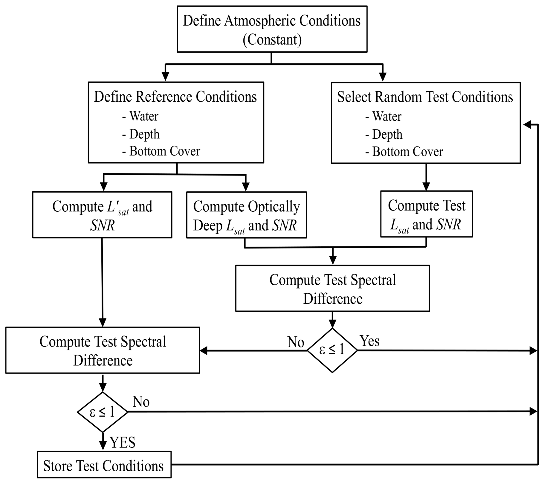
Reference conditions were compared with radiances representing other possible coral reef conditions, generated by randomly and independently adjusting water and benthic properties within realistic ranges. The advantages of this Monte Carlo approach over systematic adjustments of individual parameters are that (1) fewer computations were required to estimate parameter uncertainty, (2) all uncertainties were obtained simultaneously, and (3) all parameter interactions were included in the results. In each case, the randomly generated test spectra were compared with the reference spectrum and determined to be either indistinguishably similar or sufficiently unique based on a spectral difference criterion, ε, defined by the condition-dependent SNRs of the two signals. A flow chart of the modeling procedure is shown in Figure 1. If the reference and test spectra were indistinguishable, then the test condition was recorded and a new random test condition was generated. Random tests continued until enough indistinguishable conditions were encountered to reasonably resolve the range in parameter values. This typically required between 105 and 107 test conditions. The ensemble of indistinguishable test conditions was then used to identify the range in parameter values as a measure of detection uncertainty.
2.1. Shallow Water Light Model
Light propagation within a shallow reef environment was modeled following the original two-flow irradiance propagation concepts of Schuster [27] and adapted for a shallow ocean [28,29,30]. While all of the terms are spectrally dependent, wavelength notation λ is generally omitted for brevity and inserted as necessary for clarity.
Water remote sensing reflectance measured just above the water surface is expressed as
where sr−1 is the radiance reflectance measured just below the water surface, is the irradiance reflectance of the shallow bottom, K m−1 is the attenuation coefficient for diffuse light, the subscripts d and u refer to the downwelling and upwelling irradiance streams, respectively, and D m is bottom depth. Equation (5) propagates underwater reflectance through the air/water interface assuming a flat surface [31]. The reflectance from infinitely deep water (Equation (5b)) is approximated as a polynomial [32], where bb m−1 is the backscatter coefficient of the water mixture (pure water plus suspended particles) and a m−1 is the absorption coefficient of the water mixture (pure water plus all absorbing dissolved and particulate matter). The factors = 0.084 and = 0.125 were derived by Gordon et al. [32] through extensive Monte Carlo simulations. Diffuse attenuation (Equation (5c)) was expressed as a function of a, the total scatter coefficient of the water mixture (b m−1), and the average cosine of the irradiance stream (), according to Kirk [33]. For Kd, the attenuation of downwelling irradiance, , where is the in-water solar zenith angle. For upwelling irradiance attenuation, Ku, = 0.7.
The inherent optical properties of the water column (a, b, and bb) are defined as linear combinations of pure water (subscript w) and three primary constituents: Phytoplankton (subscript p), colored dissolved organic matter (subscript ), and suspended non-algal particulate matter (subscript d), assumed to be non-absorbing calcite;
b = bw + bp + bd, and
bb = bbw + bbp + bbd.
Pure water optical properties [34] were considered constant. Phytoplankton optical properties were spectrally dependent and defined as the product of chlorophyll concentration (Cchl mg m−3) and the chlorophyll-specific coefficients for absorption (a*chl m2 mg−1) and scatter (b*chl m2 mg−1). The spectral shapes for a*chl and b*chl were defined as the average of spectra reported by Stramski et al. [35] for laboratory cultures of phytoplankton. Absorption due to dissolved organic matter was computed as , where is the absorption at the reference wavelength λ = 450 nm [36]. Light scatter from suspended calcite particles was computed as , where g m−3 is calcite concentration and m2 g−1 is the calcite-specific scattering coefficient. For this study, = 1.034 and is based on light scatter measurements reported for calcite-dominated water within intense coccolithophore blooms [37].
Backscatter from pure water, bbw m−1, was computed according to Zhang and Hu [38] as . Backscatter from phytoplankton was estimated from data reported by Stramski et al. [35] and computed as bbp = 0.001 bp. Backscatter from suspended calcite particles was computed as bbd = 0.043 bd [37].
Benthic reflectance was computed as
where i refers to the bottom type and N is the number of types considered. The fractional benthic cover of each bottom type Bi is bounded by 0 and 1 and = 1.
Radiance received at the satellite was computed with the Tafkaa atmospheric model [39,40];
where is the extraterrestrial solar irradiance, (= 30°) is the solar zenith angle, , , and are atmospheric transmittances for downwelling and upwelling irradiance, and absorption by atmospheric gases, respectively, is the atmospheric contribution to the upwelling radiance at the satellite, and accounts for atmospheric backscattering of water reflectance.
2.2. Spectral Difference
Reference sensor noise, , was defined for an Earth surface reflectance of 5%, i.e., = 0.05, regardless of wavelength. Equation (8) was then used to compute Ltyp. Note that while was adjusted throughout the analyses for various reference conditions, Ltyp remained constant.
The spectral difference criterion, ε, was defined as the difference in the top of the atmosphere radiance representing a reference condition and a test condition relative to sensor noise. Since SNR changes with scene radiance, the joint radiance variability σ when comparing the reference radiance, , and a test radiance, , was computed as
The between-spectra difference averaged across the spectral range of interest was computed as
where N is the number of discrete spectral bands. If < 1, i.e., the average radiance difference was smaller than σ, then the two spectra were regarded as indistinguishable from system noise. Equation (10) is consistent with the z-statistic for comparing the similarity of two normally distributed populations [41].
Equation (10) does not offer an absolute measure of spectral discrimination. For example, wavelengths in the red and near-IR portions of the spectrum are absorbed at higher rates than those in the mid- and short-range portions of the visible spectrum, due to absorption by pure water. Hochberg et al. [13] noted this effect and suggested that remote sensing approaches to coral reef environments are best achieved at wavelengths shorter than 580 nm. Likewise, coral reefs ecosystems are often sources of colored dissolved organic matter [42] that increases water absorption in the blue portion of the spectrum. As ε approaches the threshold value, will generally be greater than the threshold in some portions of the spectrum, likely in the mid-visible range where light transmission is a maximum, and less than the threshold in the blue and red regions of the spectrum.
2.3. Model Scenarios
Several scenarios were considered to investigate the effects of environmental conditions on the detection uncertainty for benthic and water column properties as a function of sensor SNR (Table 2). In each scenario three reference SNR values were considered; 100, 500, and 1000. The benthic cover was defined as fractional contributions from the three primary coral reef endmembers; average brown hermatypic coral (Bc), green fleshy algae (Ba), and uncolonized calcareous sand (Bs). In addition, the average coral spectrum was compared with that of a specific coral species, Porites astreoides (Bc,p), in order to test the impact of SNR on coral species discrimination. Total benthic reflectance was computed as linear combinations of the reflectance spectra representing the specified bottom types (Figure 2) using data reported by Myers et al. [43] and collected using methods reported in Mazel [44].
Water constituent concentrations for all reference conditions were set low to represent a relatively clear water column; C′chl = 0.1 mg m−3, a′g,450 = 0.2 m−1, and C′cal = 0.3 g m−3. The conditions are similar to the least clear waters examined by Hedley and others [26]. Diffuse attenuation for this condition, expressed as the spectrally weighted Kd,
where Es is the solar and sky irradiance at the water surface, was 0.409 m−1. Test constituent concentrations were varied randomly between zero and maximum values judged to be reasonable representations of most coral reef environments; Cchl = 1.0 mg m−3, ag,450 = 1.0 m−1, and Ccal = 1.0 g m−3. These conditions span the clearest waters to be encountered within coral reef environments and episodic turbid conditions that might be encountered in close proximity to population centers. The reference bottom depth for each scenario ranged from 1 to 10 m in increments of 1 m. For test conditions D was varied randomly between 0.1 m and the maximum depth at which the test condition could be distinguished from optically deep water.
In the first scenario, S1, the objective was to compute the uncertainty in the signal representing 100% coral imposed by variability in water constituents, bottom depth, and benthic cover type. Since all parameters were allowed to vary without constraints, this scenario might in practice represent the application of remote sensing to an environment where the user has no a priori knowledge other than assumptions regarding parameter value ranges. The resulting uncertainties, therefore, represented the combined variability in all parameters. The reference benthos was defined as 100% coral cover having a reflectance equal to the average coral endmember, B′c= 1.0, and test conditions included random mixtures of Bc, Ba, and Bs.
In scenario S2, uncertainties associated with endmember benthic cover and bottom depth retrieval were investigated with the assumption that the water constituent concentrations were known. This scenario is perhaps analogous to a situation where the coral reef is rather remote with typically clear water conditions and no direct influence of degraded water quality imposed by a nearby population center. The reference conditions were identical to S1, test water conditions were set equal to the reference condition, and bottom depth and benthic cover were varied randomly across the prescribed ranges.
In scenario S3, uncertainty in benthic cover was investigated with the assumption that water clarity and bottom depth are known. This scenario is analogous to a coral reef monitoring program where water quality is measured on a frequent basis, detailed bathymetric data are available, and the objective is to detect changes in benthic cover type. The reference conditions were identical to S1, water conditions and depth were set equal to the reference conditions, and only the benthic cover was allowed to vary randomly.
In scenario S4, the impact of SNR on coral species discrimination was investigated. The reference benthic cover was assumed to be 100% coral and represented by the average coral reflectance spectra, . The test benthic conditions consisted of random mixes of the coral species Porites astreoides (Bc,p) and the benthic algae endmember (Ba). Water constituent concentration and depth were constant and equivalent to the reference conditions specified in S1.
Finally, in scenario S5, we investigated the impact of SNR on water property retrieval with knowledge of endmember benthic cover and bottom depth. As in S3, this scenario is analogous to the situation in a coral reef monitoring program where benthic cover and bottom depth have been previously mapped and the objective is to quantify changes in water quality. In addition to changes in bottom depth, this scenario was devised to test the potential impact of benthic cover on water constituent uncertainty. Two separate reference conditions were considered: 100% coral cover and 100% uncolonized sand. In both cases, benthic cover and bottom depth were held constant and equal to the reference condition and only water constituent concentrations were allowed to change independently.
3. Results
3.1. Bottom Depth
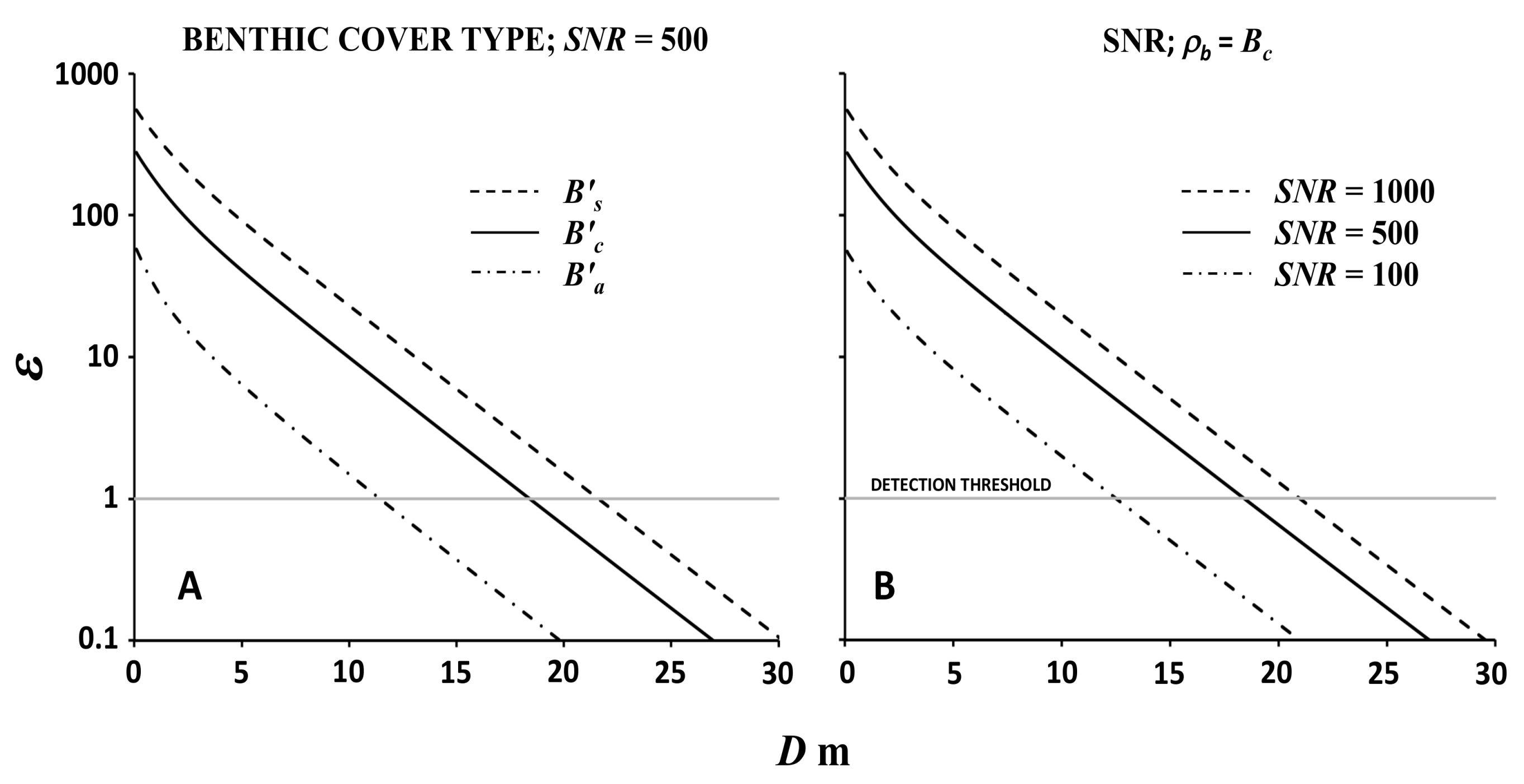
The maximum depth at which benthic cover could be detected, i.e., where ε > 1 when comparing the reference condition with the signal representing optically deep water, was affected by a combination of the concentration of water constituents (as the determinants of K), the benthic composition (that controls ρb), and the noise envelope surrounding the reference condition (defined by SNR). For example, considering SNR = 500, the extinction depths for benthic cover representing the three endmember bottom types were 18.4, 11.4, and 21.6 m for , , and , respectively (Figure 3a). The difference results from the relative contrast between the optically shallow and deep-water reflectance. The extinction depth for benthic algae was nearly half that of uncolonized sand because the spectrally averaged ρb for was more similar to and, therefore, became indistinguishable at a shallower depth compared with , which was the least similar to optically deep water. For a given bottom type (results for 100% coral cover are presented as an example), the extinction depth decreased with SNR (Figure 3b), because the envelope of uncertainty increased with sensor noise (inversely with SNR). For example, given a bottom composed of 100% coral, the extinction depth was 20.9 m for SNR = 1000 and was more than 1.5 times the extinction depth (12.6 m) under the same environmental conditions when SNR = 100.
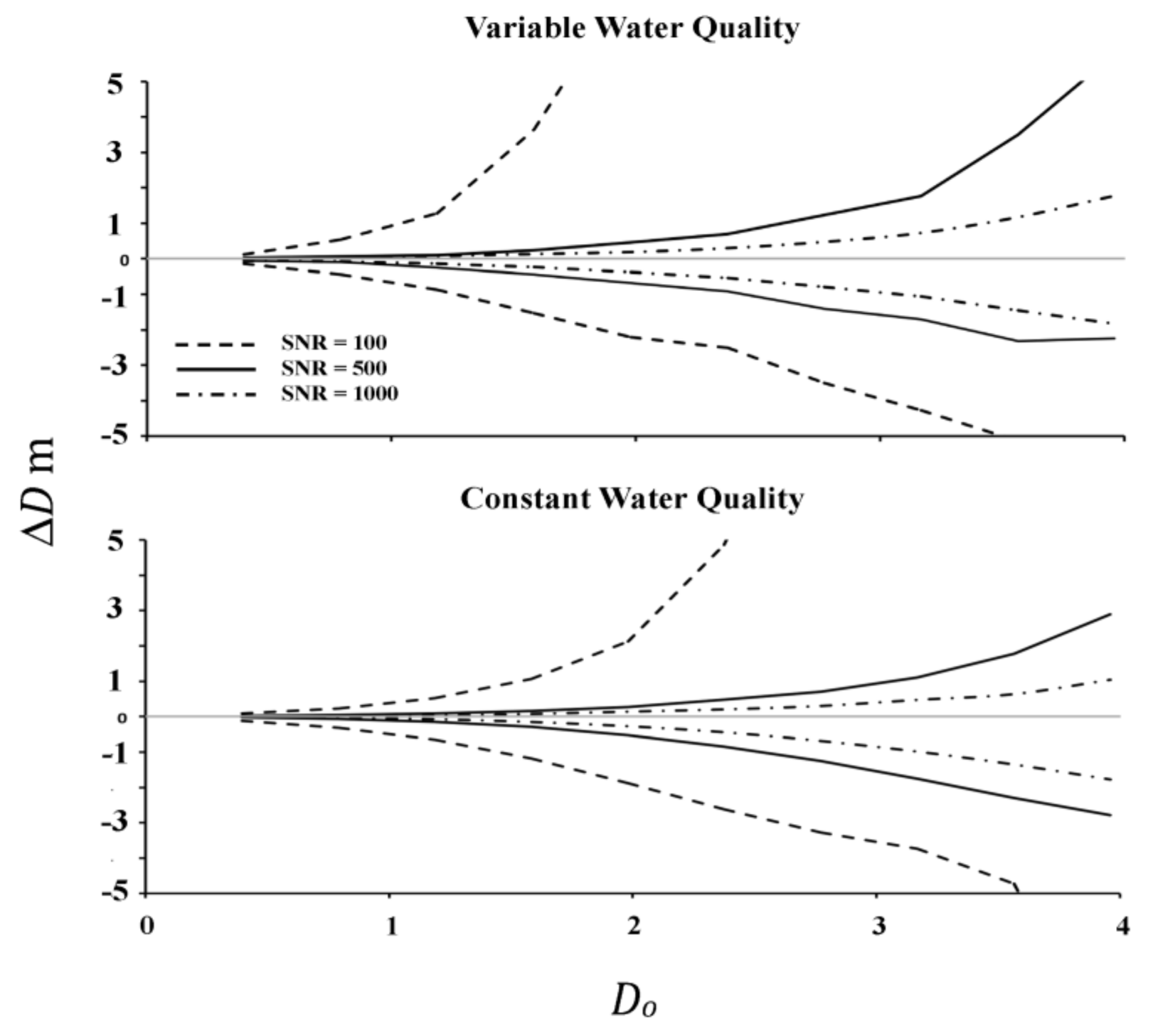
Uncertainty in the detection of bottom depth increased with increasing reference depth, expressed as the dimensionless optical depth Do (= and sensor noise, expressed as the difference between the upper and lower bounds of spectral similarity and the reference condition, ΔD (Figure 4). Positive values indicate an overestimation of D′ and negative values indicate underestimation. The rate of increase in uncertainty with respect to the reference bottom depth was greatest for SNR = 100 and progressively diminished for SNR = 500 and 1000. Retrieval uncertainty was greatest when no assumptions were made about the environment, i.e., scenario S1, where water constituent concentration was allowed to vary across the prescribed ranges. However, when water constituent concentration was constant and set equal to the reference condition (S2), uncertainty in bottom depth retrieval decreased for each of the SNR values (bottom panel in Figure 4), although uncertainty associated with SNR = 100 remained noticeably greater than for SNR = 500 and 1000.
3.2. Benthic Cover
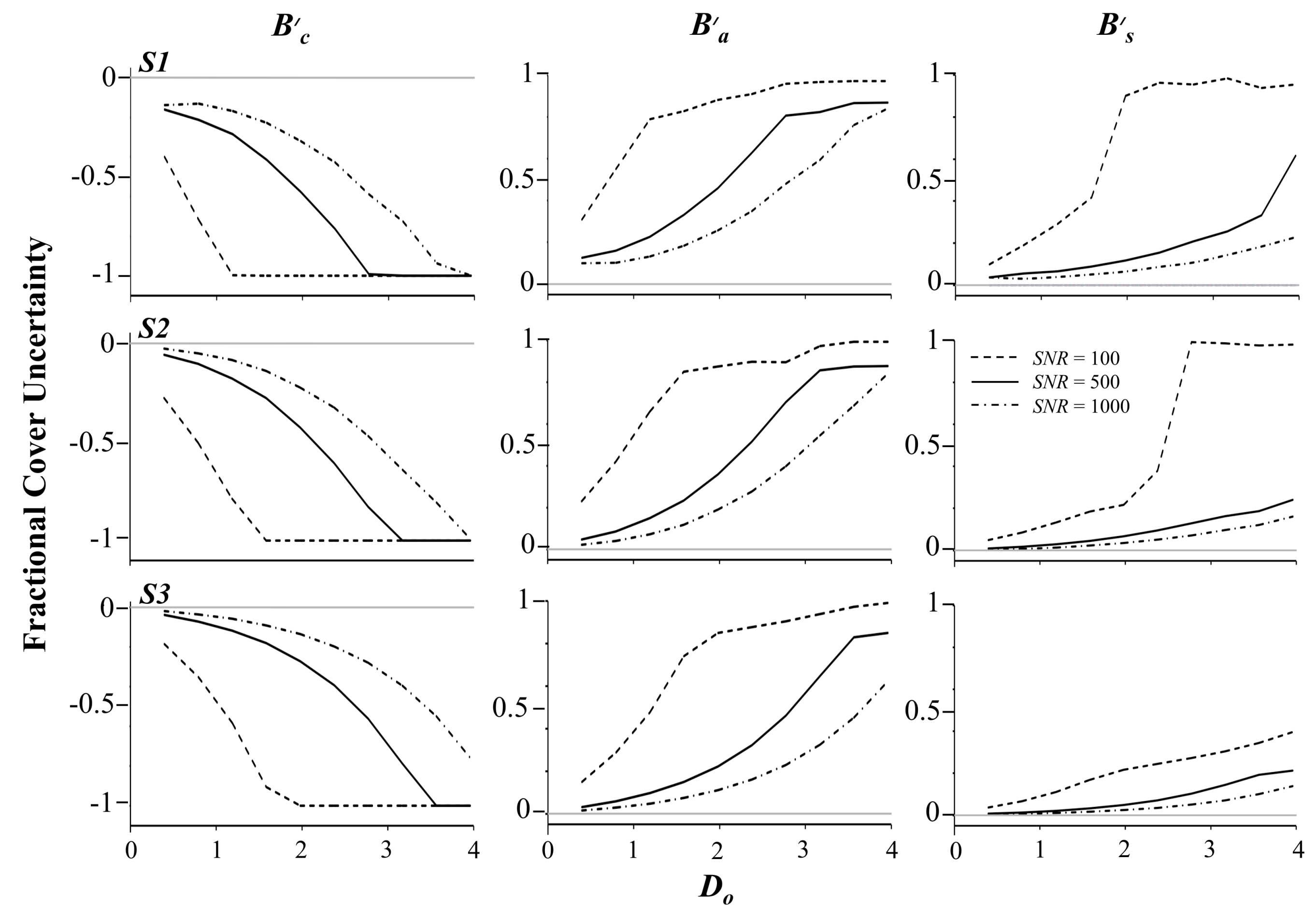
Uncertainty in the retrieval of endmember benthic cover increased with sensor noise (decreasing SNR) and the reference bottom depth (Figure 5). As the bottom depth increased, the lower confidence bound for decreased from the reference condition of 100% coral cover while and increased from the reference condition of 0% cover. Allowing water constituent concentrations and bottom depth to vary across the allowable range (S1), coral and benthic algae were indistinguishable for SNR = 100 and Do > 1.1; −1 ≤ ΔBc ≤ 0 and 0.79 ≥ ΔBa ≥ 0, where Δ indicates the difference between the upper and lower bounds of the test conditions and the reference condition. Negative values indicate under estimation of reference benthic cover while positive values indicate overestimation. Increasing SNR to 500 decreased the underestimation of to −0.28 and the overestimation of to 0.23. This trend continued as SNR increased to 1000, but the rate of change as a function of SNR was considerably less. Uncertainty in distinguishing between (or ) and was generally lower, due to a greater contrast between the vegetated and uncolonized substrates. The increase in uncertainty in benthic cover with increasing bottom depth is well understood and reported. The impact of SNR on benthic cover uncertainty was also reported by Hedley et al. [26] and expressed as the statistical overlap between specific conditions with noise applied, but their analysis did not suggest a large impact of SNR compared with environmental noise.
Constraining water constituent concentration to the reference condition (S2) resulted in a decrease in uncertainty in benthic cover detection regardless of SNR. For example, when Do = 1.1, underestimation of decreased from the S1 values to −0.78 for SNR = 100, −0.18 for SNR = 500, and −0.09 for SNR = 1000. Detection uncertainty between coral and benthic algae and between vegetated and uncolonized substrates decreased similarly. Incorporating knowledge of bottom depth (S3) decreased uncertainty further; for Do = 1.1, the underestimation of decreased to −0.58, −0.12, and −0.06 for SNR = 100, 500, and 1000, respectively.
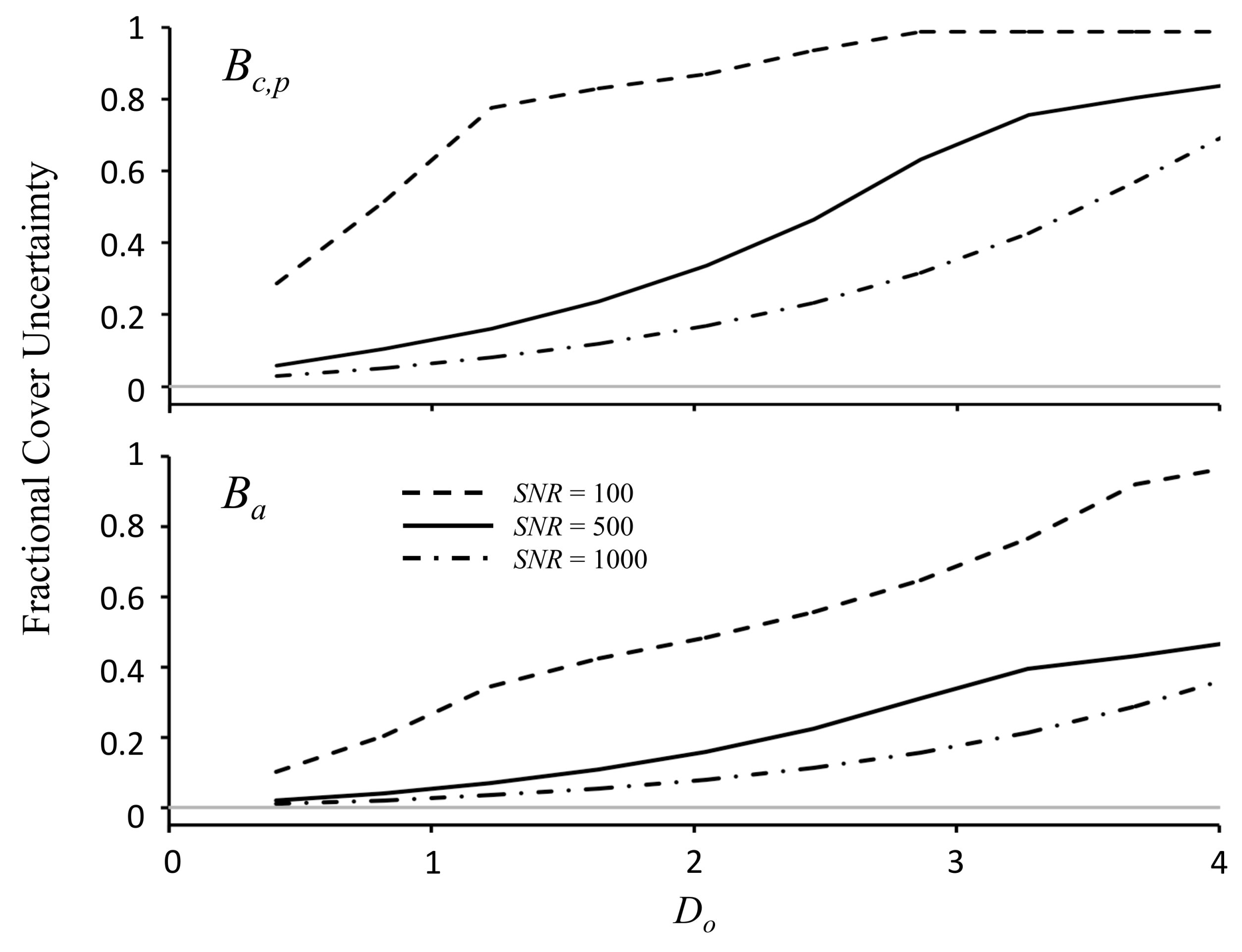
Uncertainty in distinguishing between the average coral endmember and the coral species Porites astreoides (), scenario S4, was consistently greater than the uncertainty in distinguishing between coral and benthic algae because the coral reflectance spectra were more similar to each other than the average coral and algae spectra (Figure 6). At the shallowest depths considered, D′ ≤ 3 m (Do ≤ 1.3), uncertainty in was between two and three times greater than the uncertainty in . Uncertainty increased with bottom depth and the difference in uncertainty between the coral covers and that of algae gradually diminished as the signatures from each benthic cover gradually became more similar, due to water attenuation. At the same time, detection uncertainty was significantly impacted by sensor noise. At D′ = 1 m (Do = 0.41), uncertainty in coral cover, Δ, for SNR = 100 was 0.29 relative to the reference condition = 1 (100% average coral cover). In other words, a fractional cover of 29% Porites a. was confused with 100 % average coral cover. At D′ = 2 m, the uncertainty increased to 0.52 (52% cover). However, increasing SNR to 500 significantly reduced this uncertainty to 0.06 (6%) at 1 m and 0.1 (10%) at 2 m. For SNR = 1000, uncertainty decreased slightly further to ≤0.052 (5.2%).
3.3. Water Constituents
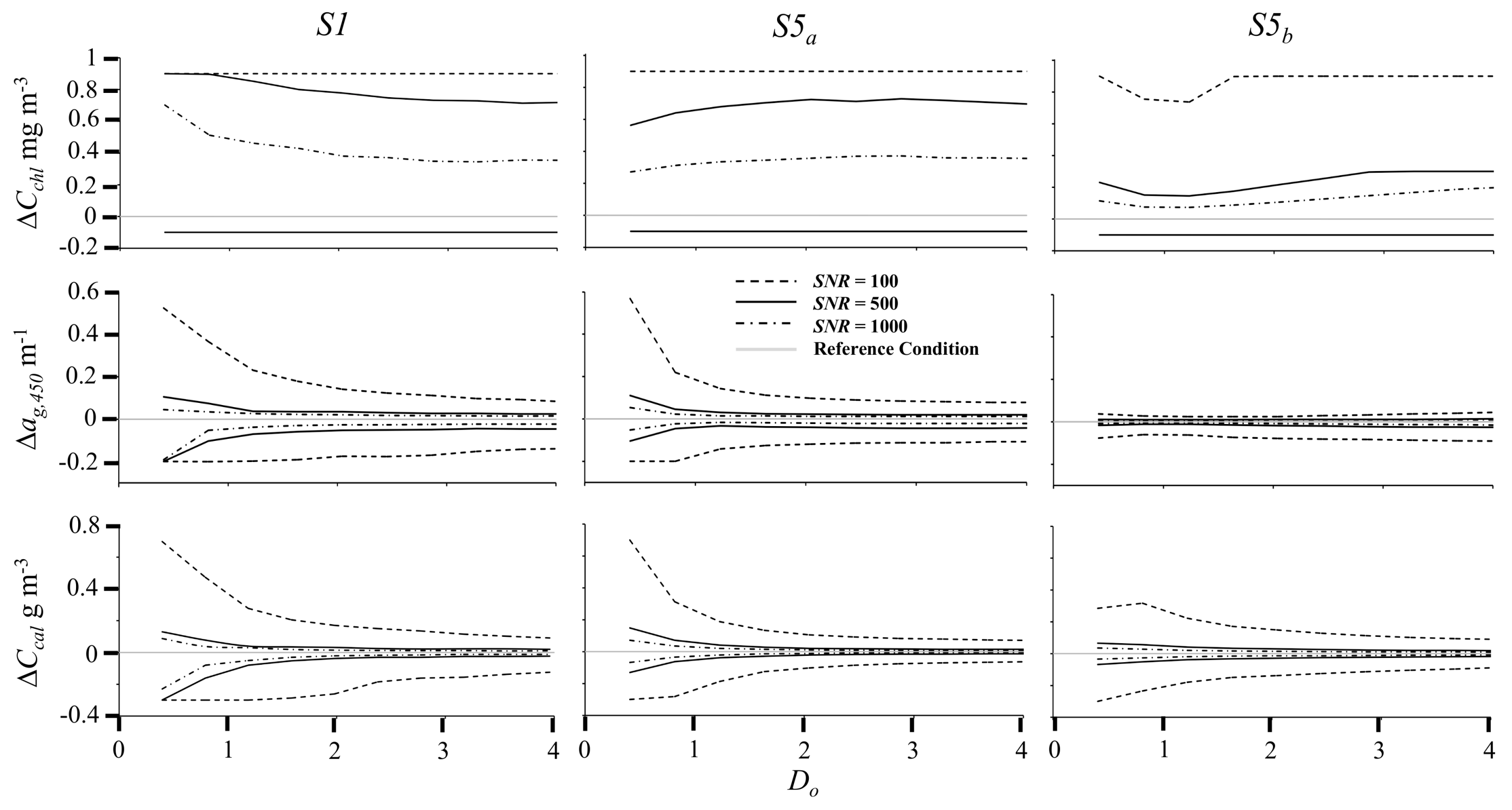
Uncertainty associated with the detection of water constituent concentration was affected by SNR, bottom depth, and benthic cover (Figure 7). Higher SNR consistently reduced detection uncertainty. However, while benthic cover uncertainty decreased with D′, uncertainty in water constituent concentration increased in shallow water, due to the diminished water signal. Both a′g,450 and C′cal were generally detectable with low uncertainty for SNR ≥ 500 and Do > 1; Δag,450 < ± 0.05 m−1 and ΔC′cal < ± 0.04 g m−3 respectively. At D′ = 1 m (Do = 0.4), retrieval uncertainty for these parameters increased significantly, especially for SNR = 100. If the benthic cover was spectrally similar to the material suspended or dissolved within the overlying water column, uncertainty increased. For example, uncertainty in the detection of chlorophyll concentration was relatively large for scenarios where the reference benthos was composed of healthy coral (in S1 and S5a), although increasing SNR did result in a modest reduction in uncertainty. This is because absorption by phytoplankton is similar to absorption by zooxanthellae, the chlorophyll-containing coral symbiont (in S5a), and the combination of coral and benthic algae (in S1). For SNR = 100, the reference concentration was indistinguishable from the entire range of test concentration, 0 ≤ Cchl ≤ 1 mg m−3. However, uncertainty in Cchl detection improved when the benthic cover was composed of uncolonized sand (in S5b). In this case, increasing SNR from 100 to 500 resulted in a significant decrease in detection uncertainty. At the same time, uncertainty in detecting Ccal was smaller when the benthic cover was coral or algae and increased when the substrate was uncolonized sand.
4. Discussion
It is shown that SNR can impose significant limitations on the ability to detect benthic cover, bottom depth, and water constituents for all but the shallowest reef conditions considered (D = 1 m). The threshold criteria for signal detection, ε = 1, essentially quantifies the average difference between a reference condition and many test conditions relative to sensor noise imposed on the two signals. If ε > (≤) 1, then the two signals are (are not) detectable as two distinct conditions. Since ε expresses the spectrally averaged difference, one should expect that ε > 1 in some parts of the spectrum while in other parts ε < 1. The criteria might, therefore, be viewed as too constraining since there will likely be unique information remaining where ε > 1. However, the amount of retrievable information will diminish as portions of the spectrum become progressively immersed within the envelope of sensor noise. Thus, ε may be viewed as a reasonable proxy for the difference between two similar spectra.
Hedley et al. [26] conducted a sensitivity analysis of sensor and environmental sources of retrieval uncertainty applied to a hypothetical airborne sensor and concluded that SNR had only a limited influence on the overall uncertainty relative to environmental sources. While many environmental sources, such as atmospheric constituent concentration and glint from a wind-roughened water surface, can easily exceed those associated with SNR, such uncertainty is often spectrally correlated in ways that are well understood and, therefore, can be mitigated. SNR, on the other hand, forms the foundation of irreconcilable uncertainty to which environmental sources of uncertainty are added. It is, therefore, prudent to make sensor development decisions with knowledge of how SNR impacts the overall uncertainty in the retrieval of key environmental parameters.
From an optical remote sensing perspective, one of the strongest indicators of coral health is bleaching; a brightening of the coral host, due to the absence of the microalgal symbiont, zooxanthellae [44]. When present in healthy coral, absorption by photosynthetic pigments contribute largely to the overall reduction in coral reflectance relative to the calcium carbonate foundation secreted by the coral host. During a bleaching event, the zooxanthellae vacate the coral host and the overall reflectance of the coral increases and takes on an appearance more similar to uncolonized calcareous sediment. Remote detection of bleaching is similar to the problem of estimating healthy coral cover when surrounded by uncolonized sand, illustrated in scenarios S1, S2, and S3. For SNR = 100, the difference between the maximum and minimum confidence bounds in the detection of uncolonized sand at the shallowest depths considered, D′ = 1 m, ranged from 0.1 (S1) with unconstrained water constituent concentration and bottom depth to 0.04 with a priori knowledge water constituent concentration and bottom depth. Increasing SNR to 1000 decreased detection uncertainty by an order of magnitude. The probability of detecting a bleaching event, assuming that the reflectance of bleached coral is similar to uncolonized sand, and the resulting change in the fraction of healthy coral cover would be reasonably high given these uncertainty limits. However, uncertainty increases with bottom depth for all SNRs considered, particularly for SNR = 100. In addition to SNR the likelihood of detecting a bleaching event depends on the contrast between healthy and bleached coral. Bleached coral is not always as bright as the surrounding uncolonized sand [13] and the fraction of symbiont loss does not always scale with reflectance [45,46]. Therefore, the uncertainty estimates with regard to bleaching are likely optimistic.
The joint retrieval of both benthic cover and water constituent information is problematic, regardless of SNR. The least uncertainty in water constituent concentration occurred in optically deep water where the effects of benthic cover were minimal, but the benthic cover was highly uncertain. Conversely, the most accurate detection of benthic cover occurred in optically shallow water, but uncertainty in water constituent concentration was greatest. There is perhaps a glimmer of hope for the shallow water conundrum in that water constituent uncertainty is lower when the water constituent and benthic cover result in dissimilar effects on the total water reflectance. If the water constituent material looks like the benthic cover material, uncertainty in the retrieval of either the water constituent or benthic cover is large. The converse is also true. Within shallow water, uncertainty associated with water column chlorophyll and dissolved organic matter (both results in darker water) is minimal when the bottom is composed of bright, uncolonized sand whereas uncertainty in suspended calcite sediment (which increases water reflectance) is smallest when the bottom is composed of dark coral or algae. This raises the possibility of constructing water constituent retrieval algorithms that are benthic cover specific. For example, one algorithm could potentially retrieve Cchl and ag,450 over bright, shallow features while an algorithm for retrieving Ccal could apply only to areas of dark benthic cover. Such an approach, if successful, would likely resolve spatial variability in water quality within a heterogeneous reef environment and would be an improvement over the practice of retrieving water constituent concentration from adjacent deep water signals that are then extended to the entire adjacent shallow reef. Regardless, it is important to note that SNR will have a significant impact on the detection uncertainty, especially when SNR < 500 and Do < 1.
This study suggests that SNR for shallow coral reef applications could be optimized around a value of 500. For SNR < 500, uncertainties associated with detecting changes in benthic cover type, bottom depth and water constituent concentration increase rapidly and limit remote sensing utility to the shallowest portions of a reef environment. As SNR increases beyond 500 the parameter uncertainty decreases, but at a much slower rate. Detection of coral reef benthic features, e.g., coral reef species, seagrasses, benthic algae, and uncolonized sand, has been demonstrated utilizing airborne scanning spectrometers with SNR approaching 500, computed as the top of atmosphere radiance from a clear maritime atmosphere and a 5% reflectance surface [14,15,16,17,18]. In comparison, data from the Landsat-8 Operational Land Imager (OLI) with SNR between 237 and 367 and four relatively broad visible bands have been applied to surveys of shallow reef flats [47,48] with far less effectiveness. Roelfsema et al. [49], for example, combined empirically derived geomorphic-ecological rules with OLI data to map benthic cover type to a maximum depth of 20 m at selected locations within the Great Barrier Reef system. However, the OLI imagery was only used to characterize benthic cover directly where D < 0.75 m. In the deeper reef areas, only single-band determinations were used to characterize the bottom as either uncolonized sand (light pixels) or combinations of coral, rock, and algae (dark pixels). Combined, these reports are in agreement with the range in uncertainty in benthic cover detection as a function of depth and SNR indicated in the S1, S2, and S3 scenarios.
The engineering constraints on SNR for a sensor deployed on an aircraft are very different compared with an identical sensor placed in low Earth orbit (LEO). The number of photons collected per pixel is a product of the amount of time that the pixel is viewed (integration time), the solid angle subtended by the pixel (instantaneous field of view), and the spectral sampling. The most advanced aircraft sensors to date include the Airborne Visible/Infrared Imaging Spectrometer—AVIRIS [50], and the Portable Remote Imaging Spectrometer—PRISM [51]. These sensors collect data with high spatial resolution (GSD < 10 m), fine spectral sampling and resolution (generally < 5 nm), and peak SNR ≥ 500 within the mid-visible portion of the spectrum. This is possible because the sensors can be flown at low altitude resulting in a wider field of view for a specified GSD and with slow speed resulting in longer integration time. Together, these attributes result in high photon flux per pixel. A LEO sensor orbits at an altitude of approximately 2000 km and travels with a ground speed about 28,000 km h−1. Therefore, for a specific GSD, an identical LEO sensor will collect only a fraction of the photons that would be received by an aircraft sensor for a specified GSD resulting in a lower SNR. The SNR of a LEO sensor could be increased by incorporating a larger aperture in order to collect more light, but this would also increase the manufacturing and launch costs. The design GSD, i.e., the instantaneous field of view per pixel, could be increased with minimal impact on size and weight, but this will result in coarser spatial resolution and potentially significant loss of fine scale information due to spectral mixing. Finally, the sensor could operate with lower spectral resolution, thus increasing the number of photons per spectral band, but this would lead to loss of information necessary to discriminate between spectrally dissimilar properties. Thus, there exists a well-defined SNR trade space between GSD, spectral sampling, and the cost of manufacturing and launching a LEO sensor, all of which impact the amount of retrievable environmental information.
The next generation of Earth imaging systems, motivated largely by reasoning articulated in the latest NASA Decadal Survey of Earth remote sensing needs [52], will attempt to optimize the sensor design tradeoffs in order to most effectively address concerns about coastal ecosystem responses to population and climate change [53]. Coral reefs are a key environment globally due to their high biodiversity and societal services. This study indicates that SNR is a key sensor design attribute for remote sensing in support of coral reef ecological research and management and, more generally, investigations of shallow coastal environments and that data value is diminished considerably when SNR < 500.
5. Conclusions
There are three primary conclusions of this research.
(1) SNR was found to have significant and non-linear impacts on the uncertainty in detecting change in key environmental parameters associated with shallow coral reef systems (bottom depth, benthic cover, and the concentration of particulate and dissolved materials within the water column). In general, uncertainty decreased with increasing SNR and the rate of change in uncertainty per incremental change in SNR was greatest for SNR < 500. Increasing SNR from 100 to 500 resulted in significant decreases in parameter uncertainty, but increasing SNR further to 1000 resulted in only modest improvements in uncertainty.
(2) Regardless of SNR, benthic cover uncertainty increased with bottom depth as reported by previous researchers. However, uncertainty in water constituent concentration increased with decreasing water depth, particularly when the geometric depth was less than 1 optical depth. For Do > 1, uncertainty associated with ag,450 and Ccal was relatively small for SNR ≥ 500. Uncertainty in the Cchl was high regardless of SNR for all scenarios except when the benthic cover was 100% uncolonized sand and SNR ≥ 500. Regardless, retrieval of water constituent concentration in shallow water is problematic.
The sensitivity of uncertainties in water constituent concentrations to benthic cover is unrelated to SNR, but nonetheless is impacted by sensor noise. The results suggest that it may be possible to retrieve water constituent concentration in shallow water environments by parsing the imagery based on benthic brightness, where algorithms developed for absorbing matter, such as chlorophyll and dissolved organic matter, might be better retrieved over areas of high benthic reflectance, such as uncolonized sand, while the concentration of highly scattering suspended particulate matter, such as calcite sediment, may be better retrieved in areas of dark benthic cover, such as healthy coral and algae.
(3) Lastly, given the change in parameter uncertainty with sensor noise and the likely trade-offs that will be required for the development of future spaceborne imaging systems with application to coastal ecosystems, we conclude that SNR = 500 is a reasonable sensor design goal in order to optimize the utility of such a sensor for application to shallow coral reef environments. Uncertainty in submerged feature detection and retrieval increases significantly as SNR approaches a value of 100. While this may result in significant immediate savings in sensor development and launch costs, the potential loss of environmental information may have larger societal costs in the long run. On the other hand, increasing SNR above 500 will likely result in much higher sensor development costs that will be hard to justify based on expected scientific benefits.
Author Contributions
All authors contributed significantly to the writing and/or final editing of the manuscript. S.G.A. was the lead author and was responsible for model development and analysis and writing the manuscript. W.J.M. was responsible for developing concepts of SNR. M.J.M. was responsible for defining a clear maritime atmosphere, running the Tafkaa atmospheric model.
Funding
Financial support for this project is provided by the National Aeronautic and Space Administration HyspIRI Program through grants NNH15AB471 and NNX16AB05G and the research funds provided by the U.S. Naval Research Laboratory.
Conflicts of Interest
There are no conflicts of interest on the part of any of the authors.
Mathematical Symbols, Units, and Definitions
| Symbol | Unites | Definition |
| a | m−1 | Absorption coefficient for water and all impurities |
| b | m−1 | Scattering coefficient for water and all impurities |
| bb | m−1 | Backscattering coefficient for water and all impurities |
| B | Fraction of benthic cover | |
| c | m s−1 | Speed of light |
| C | mass m−3 | Water constituent concentration |
| D | m | Bottom depth |
| Do | Optical depth | |
| Eo | W m−2 nm−1 | Extraterrestrial solar irradiance |
| h | J s | Planck’s constant |
| K | m−1 | Diffuse light attenuation coefficient |
| m−1 | Spectrally weighted diffuse attenuation coefficient | |
| Lsat | W m−2 nm−1 sr−1 | Earth radiance received by a satellite sensor |
| Ltyp | W m−2 nm−1 sr−1 | Typical top-of-atmosphere Earth radiance |
| rrs | sr−1 | In-water remote sensing reflectance |
| Rrs | sr−1 | Above-water remote sensing reflectance |
| Atmospheric scatter of Earth surface reflectance | ||
| SNR | Signal to noise ratio | |
| Xsys | Collective remote sensor attributes | |
| Spectral-averaged radiance difference criterion | ||
| radians | Solar zenith angle | |
| λ | nm | Wavelength of light |
| μ | Average cosine of irradiance | |
| ρatm | Atmospheric reflectance due to path radiance | |
| ρb | Benthic reflectance | |
| σ | W m−2 nm−1 sr−1 | Radiance standard deviation |
| photons s−1 | Photon flux standard deviation | |
| Atmospheric transmittance | ||
| photons s−1 | Photon flux |
References
- Odum, H.T.; Odum, E.P. Trophic structure and productivity of a windward coral reef community on Eniwetok Atoll. Ecol. Monogr. 1955, 25, 291–320. [Google Scholar] [CrossRef]
- Spurgeon, J.P.G. The economic value of coral reefs. Mar. Pol. Bull. 1992, 24, 529–536. [Google Scholar] [CrossRef]
- Moberg, F.; Folke, C. Ecological goods and services of coral reef ecosystems. Ecol. Econ. 1999, 29, 215–233. [Google Scholar] [CrossRef]
- Hughes, T.P.; Baird, A.H.; Bellwood, D.R.; Card, M.; Connolly, S.R.; Folke, C.; Grosberg, R.; Hoegh-Guldberg, O.; Jackson, J.B.C.; Kleypas, J.; et al. Climate Change, Human Impacts, and the Resilience of Coral Reefs. Science 2003, 301, 929–933. [Google Scholar] [CrossRef] [PubMed]
- Kleypas, J.A.; McManus, J.W.; Menez, L.A.B. Environmental limits to coral reef development: Where do we draw the line? Am. Zool. 1999, 39, 146–159. [Google Scholar] [CrossRef]
- Anthony, K.R.N.; Kline, D.I.; Diaz-Pulido, G.; Dove, S.; Hoegh-Guldberg, O. Ocean acidification causes bleaching and productivity loss in coral reef builders. Proc. Natl. Acad. Sci. USA 2008, 105, 17442–17446. [Google Scholar] [CrossRef] [PubMed] [Green Version]
- Hoegh-Guldberg, O. The impact of climate change on coral reef ecosystems. In Coral Reefs: An Ecosystem in Transition; Dubinsky, Z., Stambler, N., Eds.; Springer: Dordrecht, The Netherlands, 2011; pp. 391–403. ISBN 978-94-007-0113-7. [Google Scholar]
- Nyström, M.; Folke, C.; Moberg, F. Coral reef disturbance and resilience in a human-dominated environment. Trends Ecol. Evol. 2000, 15, 413–417. [Google Scholar] [CrossRef]
- Knowlton, N.; Jackson, J.B.C. Shifting baselines, local impacts, and global change on coral reefs. PLoS Biol. 2008, 6, e54. [Google Scholar] [CrossRef]
- Bellwood, D.R.; Hughes, T.P.; Folke, C.; Nyström, M. Confronting the coral reef crisis. Nature 2004, 6, 827–833. [Google Scholar] [CrossRef]
- Done, T.J. Ecological criteria for evaluating coral reefs and their implications for managers and researchers. Coral Reefs 1995, 14, 183–192. [Google Scholar] [CrossRef]
- Connell, J.H.; Hughes, T.P.; Wallace, C.C. A 30-year study of coral abundance, recruitment, and disturbance at several scales in space and time. Ecol. Monogr. 1997, 67, 461–488. [Google Scholar] [CrossRef]
- Hochberg, E.J.; Atkinson, N.J.; Andréfouët, S. Spectral reflectance of coral reef bottom-types worldwide and implications for coral reef remote sensing. Remote Sens. Environ. 2003, 85, 159–173. [Google Scholar] [CrossRef]
- Louchard, E.M.; Reid, R.P.; Stephens, F.C. Optical remote sensing of benthic habitats and bathymetry in coastal environments at Lee Stocking Island, Bahamas: A comparative spectral classification approach. Limnol. Oceanogr. 2003, 48, 511–521. [Google Scholar] [CrossRef] [Green Version]
- Karpouzli, E.; Malthus, T.J.; Place, C.J. Hyperspectral discrimination of coral reef benthic communities in the western Caribbean. Coral Reefs 2004, 23, 141–151. [Google Scholar] [CrossRef]
- Goodman, J.A.; Ustin, S.L. Classification of benthic composition in a coral reef environment using spectral unmixing. J. Appl. Remote Sens. 2007, 1, 1–17. [Google Scholar] [CrossRef]
- Lesser, M.P.; Mobley, C.D. Bathymetry, water optical properties, and benthic classification of coral reefs using hyperspectral remote sensing imagery. Coral Reefs 2007, 25, 819–829. [Google Scholar] [CrossRef]
- Dekker, A.G.; Phinn, S.R.; Anstee, J.; Bissett, P.; Brando, V.E.; Casey, B.; Fearns, P.; Hedley, J.; Klonowski, W.; Lee, Z.P.; et al. Intercomparison of shallow water bathymetry, hydro-optics, and benthos mapping techniques in Australian and Caribbean coastal environments. Limnol. Oceanogr. Methods 2011, 9, 396–425. [Google Scholar] [CrossRef] [Green Version]
- Hedley, J.D.; Mumby, P.J. A remote sensing method for resolving depth and subpixel composition of aquatic benthos. Limnol. Oceanogr. 2003, 48, 480–488. [Google Scholar] [CrossRef] [Green Version]
- Botha, E.J.; Brando, V.E.; Anstee, J.M.; Dekker, A.G.; Sagar, S. Increased spectral resolution enhances coral detection under varying water conditions. Remote Sens. Environ. 2013, 131, 247–261. [Google Scholar] [CrossRef]
- Hedley, J.D.; Roelfsema, C.M.; Chollett, I.; Harborne, A.R.; Heron, S.F.; Weeks, S.J.; Skirving, W.J.; Strong, A.E.; Eakin, C.M.; Christensen, T.R.L.; et al. Remote sensing of coral reeffs for monitoring and management: A review. Remote Sens. 2016, 8, 118. [Google Scholar] [CrossRef]
- Andréfouët, S.; Berkelmans, R.; Odriozola, L.; Done, T.; Oliver, J.; Muller-Karger, F. Choosing the appropriate spatial resolution for monitoring coral bleaching events using remote sensing. Coral Reefs 2002, 21, 147–154. [Google Scholar] [CrossRef]
- Lee, C.M.; Cable, M.L.; Hook, S.J.; Green, R.O.; Ustin, S.L.; Mandl, D.J.; Middleton, E.M. An introduction to the NASA Hyperspectral Infrared Imager (HyspIRI) mission and preparatory activities. Remote Sens. Environ. 2015, 167, 6–19. [Google Scholar] [CrossRef]
- Moses, W.J.; Bowles, J.H.; Lucke, R.L.; Corson, M.R. Impact of signal-to-noise ratio in a hyperspectral sensor on the accuracy of biophysical parameter estimation in case II waters. Opt. Express 2012, 2, 4310–4330. [Google Scholar] [CrossRef] [PubMed]
- Gillis, D.B.; Bowles, J.H.; Montes, M.J.; Moses, W.J. Propagation of sensor noise in oceanographic hyperspectral remote sensing. Opt. Exp. 2018, 26, A818–A831. [Google Scholar] [CrossRef] [PubMed]
- Hedley, J.D.; Roelfsema, C.M.; Phinn, S.R.; Mumby, P.J. Environmental and sensor limitations in optical remote sensing of coral reefs: Implications for monitoring and sensor design. Remote Sens. 2012, 4, 271–302. [Google Scholar] [CrossRef]
- Schuster, A. Radiation through a foggy atmosphere. Astrol. J. 1905, 21, 1–22. [Google Scholar] [CrossRef]
- Philpot, W.D.; Ackleson, S.G. Remote Sensing of Optically Shallow, Vertically Inhomogeneous Waters: A Mathematical Model; DEL-SG-12-81; Delaware Sea Grant Collage Program, University of Delaware: Newark, DE, USA, 1981; pp. 283–299. [Google Scholar]
- Maritorena, S.; Morel, A.; Gentili, B. Diffuse reflectance of oceanic shallow waters: Influence of water depth and bottom albedo. Limnol. Oceanogr. 1994, 39, 1689–1703. [Google Scholar] [CrossRef] [Green Version]
- Ackleson, S.G.; Smith, J.P.; Rodriguez, L.M.; Moses, W.J.; Russell, B.J. Autonomous coral reef survey in support of remote sensing. Front. Mar. Sci. 2017, 4, 325. [Google Scholar] [CrossRef]
- Lee, Z.P.; Carder, K.L.; Mobley, C.D.; Steward, R.G.; Patch, J.S. Hyperspectral remote sensing for shallow waters: 2. Deriving bottom depths and water properties by optimization. Appl. Opt. 1999, 38, 3831–3843. [Google Scholar] [CrossRef]
- Gordon, H.R.; Brown, O.B.; Evans, R.H.; Brown, J.W.; Smith, R.C.; Baker, K.S.; Clark, D.K. A semianalytic radiance model of ocean color. J. Geophys. Res. 1988, 93, 10909–910924. [Google Scholar] [CrossRef]
- Kirk, J.T.O. Dependence of relationship between inherent and apparent optical properties of water on solar altitude. Limnol. Oceanogr. 1984, 29, 350–356. [Google Scholar] [CrossRef] [Green Version]
- Pope, R.M.; Fry, E.S. Absorption spectrum (380–700 nm) of pure water. II. Integrating cavity measurements. Appl. Opt. 1997, 36, 8710–8723. [Google Scholar] [CrossRef] [PubMed]
- Stramski, D.; Bricaud, A.; Morel, A. Modeling the inherent optical properties of the ocean based on the detailed composition of the planktonic community. Appl. Opt. 2001, 40, 2929–2945. [Google Scholar] [CrossRef] [PubMed]
- Bricaud, A.; Morel, A.; Prieur, L. Absorption by dissolved organic matter of the sea (yellow substance) in the UV and visible domains. Limnol. Oceanogr. 1981, 26, 43–53. [Google Scholar] [CrossRef]
- Ackleson, S.G.; Balch, W.M.; Holligan, P.M. Response of water-leaving radiance to particulate calcite and chlorophyll-a concentrations: A model for Gulf of Maine coccolithophore blooms. J. Geophys. Res. 1994, 99, 7483–7499. [Google Scholar] [CrossRef]
- Zhang, X.; Hu, L. Estimating scattering of pure water from density fluctuation of the refractive index. Opt. Express 2009, 17, 1671–1678. [Google Scholar] [CrossRef] [PubMed]
- Gao, B.; Montes, M.J.; Ahmad, Z.; Davis, C.O. Atmospheric correction algorithm for hyperspectral remote sensing of ocean color from space. Appl. Opt. 2000, 39, 887–896. [Google Scholar] [CrossRef]
- Montes, M.J.; Gao, B.-C.; Davis, C.O. NRL Atmospheric Correction Algorithms for Oceans: Tafkaa User’s Guide; NRL/MR/7230-04-8760; The U.S. Naval Research Laboratory: Washington, DC, USA, 2004. [Google Scholar]
- Devore, J.L. Probability and Statistics for Engineering and the Sciences, 9th ed.; Cengage Learning: Boston, MA, USA, 2016; pp. 1–225. ISBN 978-1-305-25180-9. [Google Scholar]
- Boss, E.; Zaneveld, J.R.V. The effect of bottom substrate on inherent optical properties: Evidence of biogeochemical processes. Limnol. Oceanogr. 2003, 48, 346–354. [Google Scholar] [CrossRef] [Green Version]
- Myers, M.R.; Hardy, J.T.; Mazel, C.H.; Dustan, P. Optical spectra and pigmentation of Caribbean reef corals and macroalgae. Coral Reefs 1999, 18, 179–186. [Google Scholar] [CrossRef]
- Baker, A.C.; Glynn, P.W.; Riegl, B. Climate change and coral reef bleaching: An ecological assessment of long-term impacts, recovery trends and future outlook. Estuar. Coast. Shelf Sci. 2008, 80, 435–471. [Google Scholar] [CrossRef]
- Mazel, C.H. Measurement of spectral fluorescence and reflectance of benthic marine organisms and substrates. Opt. Eng. 1997, 36, 2612–2617. [Google Scholar] [CrossRef]
- Enríquez, S.; Méndez, E.R.; Iglesias-Prieto, R. Multiple scattering on coral skeletons enhances light absorption by symbiotic algae. Limnol. Oceanogr. 2005, 50, 1025–1032. [Google Scholar] [CrossRef] [Green Version]
- Morfitt, R.; Barsi, J.; Levy, R.; Markham, B.; Micijevic, E.; Ong, L.; Scaramuzza, P.; Vanderwerff, K. Landsat-8 Operational Land Imager (OLI) radiometric performance on-orbit. Remote Sens. 2015, 7, 2208–2237. [Google Scholar] [CrossRef]
- El-Askary, H.; Abd El-Mawla, S.H.; El-Hattab, M.M.; El-Raey, M. Change detection of coral reef habitats using Landsat-5 TM, Landsat 7 ETM, and Landsat 8 OLI data in the Red Sea (Hurghada, Egypt). Int. J. Remote Sens. 2014, 35, 2327–2346. [Google Scholar]
- Roelfsema, C.; Kovacs, E.; Ortiz, J.C.; Wolff, N.H.; Callaghan, D.; Wettle, M.; Ronan, M.; Hamylton, S.M.; Mumby, P.J.; Phinn, S. Coral reef habitat mapping: A combination of object-based image analysis and ecological modeling. Remote Sens. Environ. 2008, 27–41. [Google Scholar] [CrossRef]
- Green, R.O. Lessons and key results from 30 years of imaging spectroscopy. In Imaging Spectrometry XIX, Proceedings of SPIE 9222, San Diego, CA, USA, 17–21 August 2014; SPIE: Bellingham, WA, USA, 2014. [Google Scholar] [CrossRef]
- Mouroulis, P.; Van Gorp, B.; Green, R.O.; Dierssen, H.; Wilson, D.W.; Eastwood, M.; Boardman, J.; Gao, B.; Cohen, D.; Fraklin, B.; et al. Portable remote imaging spectrometer coastal ocean sensor: Design, characteristics, and first flight results. Appl. Opt. 2014, 53, 1364–1380. [Google Scholar] [CrossRef] [PubMed]
- National Academies of Sciences, Engineering, and Medicine. Thriving on Our Changing Planet: A Decadal Strategy for Earth Observation from Space; The National Academies Press: Washington, DC, USA, 2018. [Google Scholar] [CrossRef]
- Muller-Karger, F.E.; Hestir, E.; Ade, C.; Turpie, K.; Roberts, D.A.; Siegel, D.; Miller, R.J.; Humm, D.; Izenberg, N.; Keller, M.; et al. Satellite sensor requirements for monitoring essential biodiversity variables of coastal ecosystems. Ecol. Appl. 2018, 28, 749–760. [Google Scholar] [CrossRef] [PubMed] [Green Version]
Figure 1.
Computation flow chart. SNR, signal to noise ratio.

Figure 2.
Benthic reflectance spectra used in model computations.

Figure 3.
Average spectral difference parameter, ε, as a function of depth, where L′sat representing shallow reef conditions is compared with optically deep water. The water column is relatively clear (C′chl = 0.1 mg m−3, a′g,450= 0.2 m−1, and C′cal = 0.3 g m−3) and the threshold of spectral separation is ε = 1.0 (gray line). Impacts of cover type (A) are shown for B′c (solid), B′a (dot-dash), and B′s (dash) and the response to SNR (B) is shown for B'c, where SNR = 100 (dot-dash), 500 (solid), and 1000 (dash).

Figure 4.
Uncertainty in water depth (ΔD), expressed as the difference between the upper and lower bounds of the test conditions relative to the reference condition, plotted against optical depth (Do) for variable water constituent concentration (S1, upper figure) and constant constituent concentration (S2, lower figure).

Figure 5.
Uncertainty in the detection of endmember benthic cover relative to the reference condition, indicated as zero on the ordinate in each graph. S1 (top row of graphs) represent variable water constituent concentration and depth across the allowable ranges. S2 (middle row of graphs) represent variable depth while setting water constituent concentration constant and equal to the reference condition. S3 (bottom row of graphs) represent depth and water constituent concentration constant and equal to the reference condition.

Figure 6.
Detection uncertainty in the fractional cover of Porites () and benthic algae () relative to the reference condition (scenario S4, = 1). The uncertainty in the fractional cover is expressed as the difference between the upper bound of the test condition and the reference condition (solid gray line). Note that uncertainty in this scenario can only be positive (overestimated), since in this scenario and are zero.

Figure 7.
Water constituent uncertainty (y-axis) for variable depth and benthic cover (S1) and water depth and benthic cover equal to the reference condition (S5a and S5b). Scenario S5a represents benthic cover of 100% coral and S5b represents 100% uncolonized sand. The ordinate scale represents the difference between the upper and lower boundaries of parameter uncertainty, within the ranges specified, and the reference condition, indicated as 0 in all graphs.


Table 1.
Atmospheric parameter definitions and quantities representing a clear maritime atmosphere used in all model computations.
Table 1.
Atmospheric parameter definitions and quantities representing a clear maritime atmosphere used in all model computations.
| Parameter | Quantity |
|---|---|
| Aerosol model | Maritime |
| Aerosol relative humidity | 90% |
| Aerosol optical depth (550 nm) | 0.06 |
| Atmospheric model | Tropical |
| Precipitable water vapor | 5.0 cm |
| Ozone | 0.34 atm-cm |
| Solar zenith angle | 30o |
| Sun-earth distance | 149.6 × 10⁹ km |
Table 2.
Summary of Scenario Conditions.
| Global Scenario Reference Conditions SNR = 100, 500, 1000 | ||||
|---|---|---|---|---|
| Scenario | Benthic Cover | Bottom Depth | Water Constituents | |
| S1 | 0 ≤ Cchl ≤ 1 mg m−3 0 ≤ ag,450 ≤ 1 m−1 0 ≤ Ccal ≤ 1 g m−3 | |||
| S2 | *OD = Optically Deep | mg m−3 m−1 g m−3 | ||
| S3 | ||||
| S4 | ||||
| S5 | S5a | S5b | 0 ≤ Cchl ≤ 1 mg m−3 0 ≤ ag,450 ≤ 1 m−1 0 ≤ Ccal ≤ 1 g m−3 | |
© 2018 by the authors. Licensee MDPI, Basel, Switzerland. This article is an open access article distributed under the terms and conditions of the Creative Commons Attribution (CC BY) license (http://creativecommons.org/licenses/by/4.0/).
Share and Cite
MDPI and ACS Style
Ackleson, S.G.; Moses, W.J.; Montes, M.J. Remote Sensing of Coral Reefs: Uncertainty in the Detection of Benthic Cover, Depth, and Water Constituents Imposed by Sensor Noise. Appl. Sci. 2018, 8, 2691. https://doi.org/10.3390/app8122691
AMA Style
Ackleson SG, Moses WJ, Montes MJ. Remote Sensing of Coral Reefs: Uncertainty in the Detection of Benthic Cover, Depth, and Water Constituents Imposed by Sensor Noise. Applied Sciences. 2018; 8(12):2691. https://doi.org/10.3390/app8122691
Chicago/Turabian StyleAckleson, Steven G., Wesley J. Moses, and Marcos J. Montes. 2018. "Remote Sensing of Coral Reefs: Uncertainty in the Detection of Benthic Cover, Depth, and Water Constituents Imposed by Sensor Noise" Applied Sciences 8, no. 12: 2691. https://doi.org/10.3390/app8122691
Note that from the first issue of 2016, this journal uses article numbers instead of page numbers. See further details here.