Featured Application
Sediment characteristics and dynamics are studied using in situ optical measurements.
Abstract
Measurements of optical properties have been used for decades to study particle distributions in the ocean. They are useful for estimating suspended mass concentration as well as particle-related properties such as size, composition, packing (particle porosity or density), and settling velocity. Measurements of optical properties are, however, biased, as certain particles, because of their size, composition, shape, or packing, contribute to a specific property more than others. Here, we study this issue both theoretically and practically, and we examine different optical properties collected simultaneously in a bottom boundary layer to highlight the utility of such measurements. We show that the biases we are likely to encounter using different optical properties can aid our studies of suspended sediment. In particular, we investigate inferences of settling velocity from vertical profiles of optical measurements, finding that the effects of aggregation dynamics can seldom be ignored.
1. Introduction
Optical properties have long been used to study suspended particles and their dynamics (e.g., reviews by [1,2,3]). The most commonly measured optical properties are attenuation and scattering at different angles (both forward and back). Other optical devices, including ambient radiation sensors, cameras, and holographic instruments, also produce valuable data, but this paper will focus primarily on measurements of attenuation and scattering. Measurement volumes are typically small (from a few mL to tens of mL) and temporal averaging can increase the likelihood that rare large particles are sampled. Optical measurements can provide relatively direct estimates of mass or volume concentrations and particle size, and they also can be used to infer information about particle density, composition, and settling velocity. The primary advantages of using optical properties to study suspended particles are that they can be obtained at high frequency over long periods, and they are relatively non-invasive. Interpretation of optical measurements, however, are complicated by the fact that measurements are affected by all the particles in the suspension, but as we explain below, they do not respond to all particles equally. Other known disadvantages of optical instruments are that they saturate at high particle concentrations (e.g., [2]); they are intrusive and can produce turbulent wakes; they can be affected by ambient light; they can have large power demand; and they are susceptible to bio-fouling.
1.1. Optical Proxies of Properties of Sediment Particles
1.1.1. Volume and Mass Concentration
Most of the variation in optical signals measured in the field is due to changes in suspended particle mass concentrations (SPM; e.g., [4]). Optical estimates of SPM typically are made with measurements of attenuation or scattering at long visible wavelengths (e.g., 660 nm) or at infrared wavelengths (e.g., 850 nm), minimizing the impacts from varying dissolved materials and particulate absorption [5]. Transmitted light, which is reduced by scattering and absorption by particles, is measured in the near forward direction by so-called transmissometers, and scattered light can be measured at an angle near 90° by nephelometers, or at an angle greater than 90° by optical backscatter sensors (OBS). A multi-site comparison of the application of backscattering, side-scattering, and attenuation as proxies for SPM demonstrated their ability to predict SPM within 36%, 51%, and 54% respectively, for 95% of all cases [4]. The differences likely are due to variable sensitivity of each property to particle size, packing, and composition [1,6,7,8]. For example, the acceptance angle of transmissometers acts to filter out responses from larger particles [9]. SPM has also been estimated from space-based measurements of radiance (e.g., [10]). Remotely-sensed reflectance is most sensitive to the particulate backscattering coefficient in red and NIR wavelengths [11].
1.1.2. Size
Suspended sediment ranges in size from sub-µm-sized clay platelets to mm-sized sand and even larger flocs. It also encompasses plankton, non-algal organic particles, and aggregates that can be mixture of both organic and inorganic particles. We ignore in this paper particles capable of sinking at speeds >10 mm s−1. These are rarely in suspension and, when they are in suspension, concentrations may saturate optical instruments. Optical proxies for size information include size distributions inverted from measurements of near forward scattering at several angles [12], the exponents of power-law fits of the particulate attenuation or backscattering spectrum [13,14,15] (but see [16]), and the fluctuation in optical signals, which can be used to obtain the average size of suspended particles [17]. Images of particles have also been used to derive size distributions, particularly of larger flocs and aggregates (e.g., [1,3]).
Theoretically, the maximal response of attenuation or scattering per volume (equivalent to mass if density is constant) occurs for single-grain sediment near (D/λ)(n − 1) ~ 1 where λ is the wavelength in water (= 0.75λair), D is the particle diameter, and n is the index of refraction of the particle relative to water ([18], Figure 1). For solid inorganic particles with n = 1.15 at λair = 660 nm, the maximal attenuation per mass occurs for small particles with diameters between 0.8–3.2 µm. This dependency decreases as 1/D as D increases, and it increases for larger indices of refraction (Figure 1). Increases in the index of refraction are typically associated with increases in the inorganic fraction in the particle suspension [19].
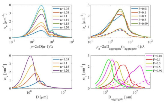
Figure 1.
Top panels: volume-specific beam attenuation (αv for solid particles (left) and aggregates (right) as function of (2πD)/λwater (n − 1) where D is diameter, λwater the wavelength in water and n the index of refraction (which increases between organic and inorganic particles). For aggregates, naggregate = 1 + F(n − 1), where F is the solid fraction and n the index of refraction of the particles that comprise the aggregate. In all cases, the volume used to compute αv is that of the solid fraction. Bottom panels: same as on top but plotted as function of particle diameter. In all the computations λair = 660 nm and n’ = 0.0001, where n’ is the imaginary part of the index of refraction, representing absorption. For aggregates we use n = 1.15 (solid) and n = 1.05 (dashed) typical of inorganic and organic materials, respectively.
The dependence of attenuation or scattering per unit of suspended mass on size should limit their use for estimation of SPM in suspensions with varying particle size, yet they are reasonably precise proxies for SPM across a range of environments, as discussed previously. This paradox is resolved if particles in suspension are not primarily single solid particles, but rather are agglomerations of particles separated by relatively large volumes of interstitial fluid and transparent organic material [1,20]. Terminology used to describe particle agglomerations in suspension can be ambiguous. Here we refer to a “floc” as an agglomeration of material that forms in suspension at relatively short times scales (e.g., tides) that is susceptible to breakup under increasing shear stress. We use the term “aggregate” to refer to an agglomeration that has undergone multiple cycles of resuspension and deposition, during which it has become more compacted and more strongly bound. While the component particles in flocs and aggregates may be similar, the density and settling velocity of aggregates is greater [21]. Flocs and aggregates typically sink faster than their component particles [22,23]. Flocs are broken by shear, including that generated by turbulence and by sinking, limiting their maximal size to about 1 cm [20,22,24,25,26]. Aggregates, because they are more compact and stronger, are not broken easily by shear. In terms of their optical properties, flocs, if sufficiently porous, can maintain the efficiency of scattering of the particles of which they are made [27], resulting in mass-specific optical properties that are independent of floc size. These theoretical results were validated in laboratory and field experiments that found that attenuation and backscattering to SPM ratios remained relatively constant despite large changes in particle size [1,28]. More densely packed aggregates theoretically should have mass-specific optical attenuation, scattering and backscattering coefficients that decrease with increasing aggregate size, but at a rate that is less than the 1/D dependence of solid particles. This theoretical relationship has not been demonstrated with measurements.
1.1.3. Composition
Composition of suspended particles ranges from inorganic clays and silts of varied mineralogy to organic particles including both pigmented phytoplankton and non-algal particles. An optical proxy for composition (separating dominance by organic and inorganic particles) is the ratio of backscattering to total scattering [29,30]. Fluid-filled organic particles such as plankton have lower indexes of refraction compared to inorganic particles, resulting in a lower backscattering relative to total scattering. The ratio of chlorophyll-containing particles to total particles, estimated from the ratio of chlorophyll absorption to the particulate beam attenuation, has also been used as a compositional proxy in locations where the particle assembly includes a significant inorganic component [31]. In addition, the ratio of particulate organic carbon to SPM was found to correlate well with the ratio of particulate absorption at 675 nm to that at 570 nm [32]. It should be noted that optically derived knowledge of composition and/or size can lead to improved estimates of particulate concentration from optical measurements and associated composition (or size)-specific algorithms relative to those that do not account for variations in particle composition and/or size [1,16,32,33].
1.1.4. Packing
A proxy for bulk particle density has been derived from the ratio of beam attenuation (a mass concentration proxy) to the total particulate volume (obtained by inverting the forward scattering measurements with the Laser In Situ Scattering and Transmission (LISST) sensor [28,34,35]). If particle volume increases due to aggregation (with a significant fluid fraction), particle density will decrease. This will happen up to the point where the particle has a fractal dimension that is reduced below two, at which point most light passes through the particle and attenuation is caused only by component particles. Because the beam attenuation is also closely linked to the summed cross-sectional area of all the particles, it follows that the above proxy should behave similarly to the suspension’s volume-to-cross-sectional-area ratio, or Sauter diameter [34].
1.2. Particle Dynamics
In this section, we focus on the bottom boundary layer (BBL; for a recent review of the fluid dynamics of the BBL see [36]). The particle assembly C is a sum of many types of particles C = ∑i Ci, each with a specific settling speed, composition, size and any other property that is relevant to either hydrodynamic or optical properties.
The general conservation equation for particles can be written as:
where Ci is the mass concentration of particles of type i, t is time, U is the 3-D velocity field, wi is the settling velocity of these particles (we use the convention that it is positive downward), K is a diffusion coefficient, f(Ci−j, Cj) represents aggregation and disaggregation dynamics creating and destroying Ci-type particles, and Si represents other sources and sinks (e.g., resuspension/deposition or biological production/consumption of particles).
To solve Equation (1) for a given flow field, one needs boundary conditions (e.g., flux or concentration of particles at the boundaries of the domain) and initial conditions (e.g., the state of the particles at time t = 0). Even then, Equation (1) cannot be solved analytically except for very simple cases such as we will address next.
Equation (1) can be simplified to represent only the vertical dimension (z, positive upwards), assuming that horizontal advection of horizontal gradients is negligible relative to vertical processes. After time averaging (or assuming steady-state), the steady balance between downward settling, upward diffusion, exchange among particle types (aggregation/disaggregation), and sources/sink is:
where Ci is the time- (and horizontally) averaged concentration of particles of type i, Keddy is an eddy diffusion coefficient (representing the mixing by the small-scale turbulent field), and wi is a constant settling velocity for each particle type i.
Large aggregation rates are associated with large particle concentrations, e.g., following a major resuspension event or during an algal bloom. Large disaggregation rates are associated with large fluid shears, e.g., in the wave boundary layer, which is a layer a few centimeters thick next to the bottom. If particle concentrations and fluid shears do not vary greatly throughout a boundary layer, then an equilibrium size distribution develops, and the aggregation and disaggregation terms cancel one another. An assumed equilibrium under certain circumstances is unlikely to emerge in bottom boundary layers, for example when near-bed wave-generated shears are much greater than current-generated shears higher in the boundary layer.
The law-of-the-wall is often invoked in the BBL, which is consistent with a linear eddy diffusivity profile where Keddy = κu∗z, and κ is von Kármán’s constant (∼0.4), and u∗ is the friction velocity (a function of BBL turbulence, e.g., due to wave and current shear). Neglecting aggregation dynamics and sources/sinks, and integrating Equation (2) in the vertical and solving the resulting differential equation results in the Rouse equation [37,38] for a homogenous population of particles of type i:
where za is a reference elevation where a particle concentration is assigned. This is one of several different analytical solutions for the balance of settling and turbulent mixing, which vary depending on assumptions about the eddy diffusivity profile [39,40]. An alternative derivation of Equation (3) using probability theory has also been proposed [41]. Equation (3) predicts a profile that is linear in log(Ci) versus log(z), and all of the other forms predict similar decreases in concentration with elevation above the bottom. Because mass concentrations can be summed, the bulk concentration profile is:
It follows that the bulk particle concentration will also decrease with height above the bottom. Note, however, that if a suspension comprises sub-populations of particle types with differing settling velocities, each will have a different vertical profile (Equation (3)), and the profile of the summed concentration will follow Equation (4), which does not, in general, follow the linear shape in log-log space. In fact, large deviations in the bulk profile from Equation (3), under steady conditions in a turbulent BBL, are likely indications that a suspension contains particles with diverse settling velocities.
1.3. An Equation for the Vertical Distribution of an Optical Property
The mass concentration of a population of particle type i is Ci = NiViρI, where ρi is individual particle density, Ni is the number concentration of particles of type i, and Vi is individual particle volume. By the Beer–Lambert law the bulk optical response (e.g., backscattering or beam attenuation) of a sub-population bx,i, is the simple sum of the individual contributions so that:
and the bulk response to the combined sub-populations is:
where αv,i, is a volume-specific optical property. Volume- or mass-specific optical properties typically are calculated by using Mie theory (which assumes homogeneous spherical particles) for solid particles, or by using other models for flocs (e.g., [31]). The calculations of αv,i require as input particle diameter, index of refraction (a function of composition), wavelength of light, and, for flocs, the fractal dimension that relates volume concentration to mass concentration. The results are resonance-like functions of size (Figure 1). Although the application of Mie solutions to backscattering has been challenged based on observations (e.g., [42]), it is reasonable to relate constant values of αv,i to specific particle types. Both Equations (5) and (6) rely on the Beer–Lambert law, with underlying assumptions that the light is monochromatic with parallel rays and, most importantly, that the particles do not scatter the light multiple times. This is clearly not the case as particle concentrations rise but, at low concentrations, we may be able to assume that Equations (5) and (6) are valid. Substituting optical response for concentration in Equation (3) yields an equation for the optical-response profile for a homogenous sub-population i with identical αv,i, Vi, and wi:
Equations (6) and (7) can be combined to yield an equation for the bulk response of a heterogeneous population:
As with particle concentrations, we find that the information provided by a profile of optical properties will depend on how heterogeneous the suspension is. Unlike the concentration profile, the averaging done by the optical properties depends on how the optics respond to different particles (Equation (8)). Hence, the more biased an optical property is towards a specific particle type, the better it can provide information on its specific settling speed.
2. Observations
Field data were obtained from a profiling instrument platform deployed at the Martha’s Vineyard Coastal Observatory (MVCO) south of Martha’s Vineyard, MA, USA, at the 12-m isobath in the summer of 2011, as part of the Office of Naval Research (ONR)-funded Optics and Acoustics and Stress In Situ (OASIS) experiment [43]. The platform was mounted on a pivoting arm that profiled every 20 min from 10 cm to 2 m above bottom. The platform was equipped with variety of optical and acoustical sensors. Here we discuss data from a Sequoia LISST 100-X (Sequoia Scientific, Bellevue, WA, USA), a EcoBB2f (WETLabs, Philomath, OR, USA) triplet measuring dissolved organic fluorescence and backscattering at two wavelengths (532 and 650 nm), and a WETLabs AC-9 spectral absorption and beam attenuation meter. Water was pumped from an intake at the tip of the arm into the 10-cm pathlength sampling volume of the AC-9. An automatic valve periodically routed the water sample through a 0.2-μm filter to remove particulates, leaving the dissolved fraction, to obtain calibration-independent particulate properties [44]. Shear velocity u∗c [cm/s] associated with mean flow in the bottom boundary layer (BBL) was inferred from a pair of acoustic Doppler velocimeter (Sontek, San-Diego, CA, USA) measurements (cf. [45]), and model estimates of the wave–current combined maximum shear velocity in the wave boundary layer (relevant to sediment resuspension) were determined using a version of the Grant–Madsen model [46,47]. We have plotted sign(u) u∗c in Figure 2, where u is the east–west component of the current velocity, to differentiate flood (east, positive) from ebb (west, negative). The location is dominated by the east–west semi-diurnal tidal currents, northward swell, and periodic storms (Figure 2). The measurements discussed here were taken in the bottom boundary layer, which is mostly well mixed.
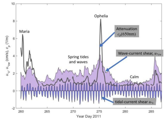
Figure 2.
Time series of conditions at the 12-m Martha’s Vineyard Coastal Observatory (MVCO) site during the Optics and Acoustics and Stress In Situ (OASIS) deployment in 2011: beam attenuation at 650 nm measured at 1 m above the bottom (gray), tidal current shear velocity sign(u)u∗c (blue), and combined wave-current shear velocity u∗cw (purple). Notice labels describing specific periods.
Waves and currents varied during the experiment, and we have selected four periods with distinctly different forcing and optical responses (Figure 2). Two periods (Maria and Ophelia) were associated with offshore passage of hurricanes and arrival of swell waves at the study site. Another period (Spring tides) was associated with moderate wave conditions and strong spring tidal currents. The fourth period (Calm) was characterized by low waves and weaker neap tidal currents. For each of the four periods identified in Figure 2, we show the distribution of the following optical properties (or properties inferred from optical measurements):
- Beam attenuation cp(650) [m−1] measured by the AC-9 and particulate backscattering coefficient (bbp(650) [m−1] measured by the EcoBB2F provide proxies of particulate concentration (e.g., [5], where higher values associated with higher particle concentrations.
- Exponent of the power-law fits of the particulate beam attenuation γcp [dimensionless] and backscattering γbbp [dimensionless] (cp = cp(λ0)(λ/λ0)−γcp, with an analogous formula for γbbp) provide proxies for size distribution in the finer sizes (e.g., [13]). Lower values are associated with larger size averaged particles. γcp is biased towards the smaller (0.5 to 10 µm) particles in the population [9], and γbbp may be more sensitive to larger particles [15].
- Sauter diameter Ds [µm] is determined from the ratio of LISST measurements of volume and area concentrations, summed over size classes i as Ds = 1.5 ∑Vi/∑Ai and reciprocal of particle density ρa−1 = ∑Vi/cp [m ppm−1 = µm], using the LISST-based cp. Both are proxies for packing: larger values of Ds indicate larger, less-dense particle populations, and larger values of ρa−1 also indicate less-dense particle populations.
- Particulate backscattering ratio bbp(532)/bp(532) measured by the EcoBB2F (bbp(532)) and by differencing of particulate attenuation and particulate absorption from the AC-9 (bp(532)) was a proxy of composition. Increasing values of this ratio are associated with inorganic particles [29,30]. For very small particles, this ratio is also sensitive to size, increasing for smaller particles.
- Chlorophyll to attenuation ratio Chl/cp(650) is another proxy of composition where higher values are associated with higher phytoplankton-based organic content [31].
- LISST-based size distribution spanning from 2–250 µm at 32 size bins and using a spherical kernel.
We selected 1-h intervals during each of the different periods identified in Figure 2 when the concentration profiles estimated from attenuation decreased monotonically with elevation above the seabed, and the profiles were relatively well approximated by a linear profile in log-log coordinates (Equation (5)). These profiles were consistent with the steady-state Rouse balance discussed above, suggesting that we might be able to neglect the effects of horizontal gradients and temporal transients. The data represent the average of three consecutive profiles, each of which took 20 min to complete. All properties are displayed as a function of elevation above the bottom in Figure 3, Figure 4, Figure 5 and Figure 6. Trends in vertical profiles and representative values (mean and standard deviation) for each time period are summarized in Table 1 and Table 2.
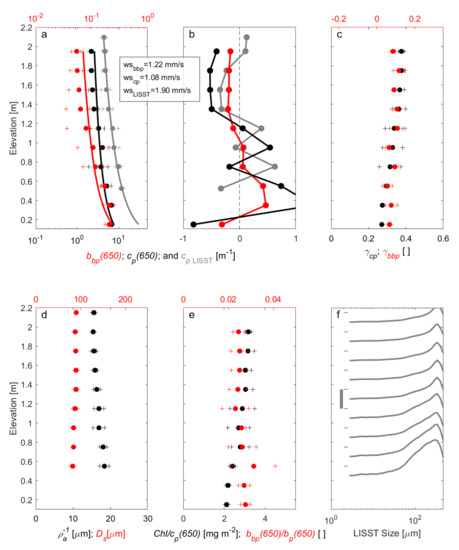
Figure 3.
Profiles of optical parameters at the MVCO site on day 261.1 when waves from Hurricane Maria were coming to shore (see Figure 2). (a) Beam attenuation (cp(650), black), particulate backscattering (bbp(650), red), and LISST attenuation (gray). (b) Deviation from the Rouse-profile fits for the same parameters (i.e., observed minus fit). (c) Power-law exponent of cp(650) (black) and bbp(650) (red). (d) Sauter diameter (red) and inverse particle density (black). (e) Ratio of chlorophyll divided by cp(650) (black) and backscattering ratio (red). (f) Spectra of LISST volume concentration as a function of size at nine elevations. In panels (a, c, d, and e), standard deviation about the mean values for three consecutive profiles (60 min) are shown with crosses. Dashed lines in panel (a) are log-log (Rouse) fits to the data. In panel (f), the elevations for each spectrum are indicated by black lines, and the gray vertical scale indicates 10 μL/L. Numbers in the box denote settling velocities based on Rouse fits to backscattering, AC-9 particulate attenuation at 660 nm, and LISST attenuation at 670 nm.
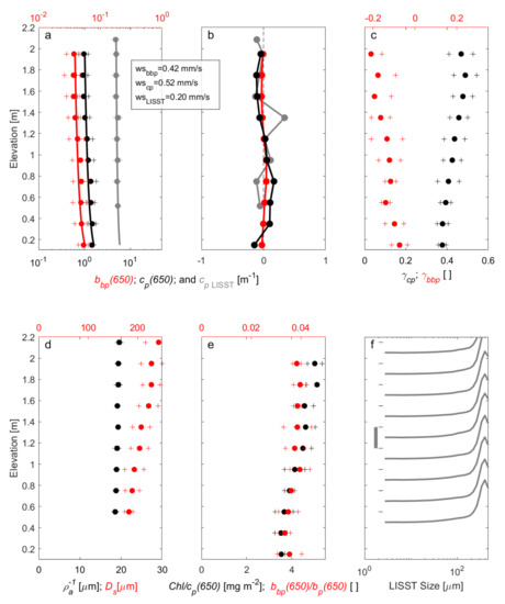
Figure 4.
Profiles of optical parameters at MVCO on day 268.62 during spring tides and moderate waves. Panels are as described in Figure 3.
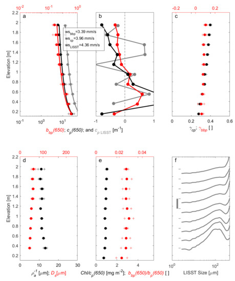
Figure 5.
Profiles of optical parameters at MVCO on day 275.20 during the passage of Hurricane Ophelia. Panels are as described in Figure 3.
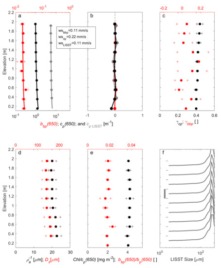
Figure 6.
Profiles of optical parameters at MVCO on day 281.93 during calm conditions. Panels are as described in Figure 3.

Table 1.
Trends in particle parameters as function of depth based on the average of three profiles in the BBL in each of the four periods denoted in Figure 2. ↘ and ↗ denote profiles that are decreasing or increasing (respectively) with elevation above the bottom, ∼ denotes that the trend is weak, and | denotes that there is no trend with elevation.
Table 2.
Mean and standard deviation (in brackets) of optical particle parameters computed based on the average of three profiles in the BBL in each of the four periods denoted in Figure 2. The wave-current and current shear velocities and the settling velocities inferred from fitting the Rouse profile to cp and bbp are also listed, with regression coefficient r2 in brackets.
3. Results
3.1. Suspended Particulate Material (SPM)
The overall concentration of SPM fluctuated through the experiment (Figure 2), as indicated by variations cp(650) (Figure 2) and bbp(650) (not shown). The time series of cp(650) at 1 m above the bottom indicates increased SPM during Maria and Ophelia, somewhat reduced SPM during the spring tides, and low SPM during the calm period. Mean values of cp(650) in the 60-min profiles ranged from about 1 m−1 during the calm period to 12 m−1 during Ophelia, when wave-induced resuspension increased SPM in the BBL. Mean values of bbp(650) generally covaried with cp(650), ranging from 0.02 m−1 to 0.30 m−1 for the same periods. The cp(650) and bbp(650) concentrations decreased with elevation, and the profiles examined here were nearly linear in log-log space (Rouse-like). However, there was typically more scatter in the profiles of bbp(650), as evidenced by their lower r2 (Table 2), especially during periods of lower concentrations.
3.2. Settling Velocities Assuming Rouse Profiles
Mean apparent settling velocities inferred from cp(650), cp,LISST and bbp(650) profiles ranged from about 0.1 to 4 mm/s. Although the settling velocities estimated from each instrument during a given period were similar, and showed similar trends over the four periods, ws,cp(650) was usually larger than ws,bbp(650). Particulate beam attenuation measured by the AC-9 is less sensitive to large, low-density particles, so settling-velocity estimates from cp(650) were likely to favor smaller, denser, faster-settling aggregates and single-grained particles. Inferred settling speeds were largest during passage of Maria and Ophelia. They were intermediate during spring tides, and they were lowest during the calm period. During passage of the two storms the residuals of the Rouse fits showed vertical structure, with negative residuals higher in the boundary layer and positive residuals lower in the boundary layer. This pattern indicates that, nearer the bed, the profiles during storms were steeper than the Rouse balance.
3.3. Size
The spectral exponents of attenuation and backscatter increased slightly with height above the bed during the calm periods and during the passage of Maria and Ophelia. During the spring tides, the spectral exponent of attenuation increased with height above the bed, but the spectral exponent of backscatter decreased with height above the bed. Values of γcp were smaller during passage of the two storms than during the calm period and during spring tides. Values of γbbp were smallest during spring tides, even taking on negative values. Values were higher during the storms, and they were scattered during the calm period.
Sauter diameter and the reciprocal of floc density generally were well correlated because they are based on similar measurements. Sauter diameter was smaller during passage of Ophelia, when it was ~50 µm, and during passage of Maria, when it was ~100 µm. During the spring tides, Sauter diameter was largest, with diameters ~200 µm. During the calm period, Sauter diameter was ~150 µm. During Maria, the spring tides, and the calm period, inverse densities were similar and equal to ~20 µm. Values were ~10 µm during the passage of Ophelia. During the passage of the two storms, inverse density and Sauter diameter values diverged near the bed, and during the spring tides, they diverged higher in the boundary layer.
Size distributions from the LISST provide a more complete understanding of the vertical and temporal changes in size distribution. During the calm period and during spring tides, the size distributions had well-defined modes at the upper end of the LISST range. The widths of the modes were relatively constant with height above the bed during the calm period, but they were wider nearer the bed during the spring tide period. During passage of Maria, distributions were unimodal, but they were more skewed to smaller sizes than during the calmer periods. During passage of Ophelia, curious bi-modal distributions emerged. One mode was centered on diameters of ~100 µm, and the other was located in the largest diameter class. This coarser mode was dominant farther away from the bed, and the finer mode grew larger nearer the bed.
3.4. Composition
The backscattering ratio was relatively high (>0.02) during the full deployment, indicating that the suspensions were dominated by inorganic particles. The ratio was smaller during the passage of the two storms than it was during the spring tides. The backscatter ratio was not correlated to the Chl/cp ratio, which increased away from the bed in each period, consistent with chlorophyll-containing particles being at lower concentration relative to other particles closer to the bed. Chlorophyll profiles typically showed no trend with elevation (not shown), consistent with the hypothesis that the increase in the Chl/cp ratio away from the bed was due to enrichment in faster-settling non-algal particles near the bottom.
4. Discussion
4.1. Inferences from Optical Properties
The vertical profiles of the attenuation and backscattering coefficients were fit reasonably well by Rouse profiles, and the estimated settling velocities increased with increasing shear stresses, as expected. The magnitudes of the estimated settling velocities are within ranges expected for flocs and for the fine sands typical of the seabed at the MVCO site. The ~0.1 mm s−1 estimated settling velocities during the calm period were small, and they indicate material that behaved as slowly sinking washload that is evenly distributed throughout the boundary layer. The ~0.4 mm s−1 estimated settling velocities during the spring tides are in the range of typical floc-settling velocities, and the ~1 mm s−1 estimated settling velocities during the passage of Maria are typical of flocs (e.g., [48]). The ~4 mm s−1 observed during the passage of Ophelia are larger than typical floc-settling velocities, but they are representative of very fine sand (D = ~80 µm; [49]) or densely packed aggregates [21].
Interestingly, boundary shear stresses during passage of Maria were similar to boundary shear stresses during the spring-tide period, yet the estimated settling velocities were more than two times larger during Maria. Residual plots of the Rouse fits indicate that the profiles had smaller gradients (lower settling velocities) during spring tides than the profiles near the bed during passage of Maria. In addition, Sauter diameters were smaller during passage of Maria, as were the spectral exponents of attenuation. Particle size was inverted during the spring tides, with larger particles farther above bottom. The spectral exponent of backscattering was lower during the spring tides than during passage of Maria, and it decreased with height above bottom.
Despite the similar stresses during these two periods, these observations suggest different particle dynamics. The larger Sauter diameters, inverted particle size, and smaller values of γbbp are consistent with the hypothesis that flocs dominated the suspension during the spring tides. The flocs were fragile, and they were disrupted near the bed, but they were able to reform higher in the boundary layer. The breakage of flocs near the bed decreased bulk estimated settling velocities from the profiles by transferring mass near the bed from faster-sinking large flocs (~1 mm s−1) into slower-sinking smaller flocs or single grains. Overall, however, the extensive packaging of small particles into large flocs during spring tides was associated with small values of γbbp [15]. During the passage of Maria, we hypothesize that higher bottom shear stresses associated with the larger swell caused resuspension of fine sand typical of the site (D = ~125 µm; [50]) and caused a greater degree of floc breakup. Resuspension of sand caused larger gradients in optical properties near the bed. Resuspended sand also can account for the broadened peak in the particle size distributions. Greater floc breakup can account for smaller values of γcp during passage of Maria, because particle mass was transferred out of large flocs that were not sensed by the AC-9 into smaller flocs or single grains that were [15]. It can also account for large values of γbbp [15].
During passage of Ophelia, when stress was highest, particle sizes were smallest. This result suggests that floc breakup was more extensive during Ophelia (e.g., [26]). The finer mode in the LISST size distributions was similar to the fine sands at the site (D = ~125 µm), and the presence of this sand, with typical settling velocities of 8 mm s−1 [51], steepened the near-bed profiles of the optical properties. The appearance of the coarser mode at the upper limit of the LISST size range, however, is not consistent with greater floc breakup. We hypothesize that these particles were resuspended bed aggregates that were tougher than flocs and not prone to breakup (cf. [21]). The fact that they were relatively more abundant higher above the bottom suggests that they had settling velocities smaller than that of the fine sands (<8 mm s−1), consistent with the estimated settling velocities in the outer part of the profile of 4 mm s−1.
The hypothesis of sand resuspension during passage of the two storms can be reconciled with observed variations in the backscatter ratio, which was lower during passage of the two storms than it was during the period of spring tides. Permeable sand beds can store organic matter in the interstitial pore spaces [52]. We propose that during resuspension events, this organic material was resuspended, which caused backscatter ratios to decrease. The observation that the Chl/cp ratio did not change indicates that the organic matter in the bed interstices was degraded and did not contain chlorophyllous material.
The relative magnitudes of Sauter diameter and inverse density in the different periods may also argue for different particle dynamics during passage of the storms. During these periods, the ratios of Sauter diameter to inverse density were smaller than during the periods of spring tides and calm. This ratio reduces to the ratio of the beam attenuation coefficient measured by the LISST to the particle area estimated by the LISST. The inversion of near-forward scattered light measured by the LISST to particle area assumes that a single refractive index applies to all particles. We hypothesize that small organic particles liberated from the bed during resuspension had attenuation to particle area ratios that were smaller than the ratios for particles during the spring tides and during the calm period.
4.2. Broader Advantages and Disadvantages of Optical Measurements
Measurements of optical properties often behave in ways consistent with our expectations. When they do, their advantages are that they provide robust, relatively non-intrusive, well-understood first-order information about the suspended particle populations. Their main disadvantages are their sensitivity to ambient light and limitations in turbid conditions, tendency to foul, and, in some cases, their large size, power requirements, or data storage limits. The more subtle disadvantages are the biases that each instrument has, often based on wavelength, angles of illumination, or acceptance angles. These disadvantages can be turned to advantage by using combinations of different measurements, each with a different bias, as we have shown here. Combinations of optical measurements (attenuation and backscatter at various wavelengths, measurements of chlorophyll, size data from the LISST) provide more information about the size and composition of the particle population.
Simple, time-tested optical measurements such as attenuation and backscatter remain valuable, even in complicated settings like MVCO. Their main advantage is they yield simple interpretations in terms of SPM that capture the first-order variations that often can be linked to wave- and current-induced bottom stress. The main disadvantages are that they can be biased by size and composition, and the conversion from attenuation or backscatter to SPM can vary, depending on instruments, particle size, composition [1,2].
The advantages of direct measurements of size from the LISST are clear: they provide information that cannot be measured directly with simpler optical sensors, and the size information is very useful for interpreting the dynamic behavior of the particles. One important disadvantage is that LISST instruments are large and intrusive. In addition, they have upper limits on sizes and, when larger particles are present, they can bias results by elevating reported volumes in smaller size classes [53]. Finally, when flocs are present, the LISST may be sensitive to smaller component particles, leading to over-representation of microflocs when macroflocs are present [54].
Near-bottom profiles of optical properties allow the observations of particle populations to be interpreted in terms of sediment dynamics. In particular, near-bottom profiles of size from the LISST have not been previously reported, and offer the advantage of direct observations of size changes in a region with strong gradients in concentration and turbulent shear.
The nearly-ubiquitous appearance of Rouse-like profiles in optical measurements provides estimates of settling velocity that can be linked to particle size. The disadvantage of these interpretations is that the bulk profile can be confounded by changes in particle density (and therefore settling velocity) or skewed by overlapping profiles of diverse particle populations with varying vertical distributions. In all the cases illustrated here, relatively good Rouse fits provided settling-velocity estimates, but they could vary by an order of magnitude between profiles. Additional information was required to evaluate the underlying particle dynamics, and both floc dynamics and resuspension were found to be important.
Addition of acoustical measurements [55] could further constrain the particle dynamics and distribution as their sensitivity to composition, size, and packing differs from optical measurements. For example, for acoustic backscattering in the MHz frequency range, aggregation decreases the signal [56] while being sensitive to large single-grain particles (whereas the optical response is not).
Models of resuspension and settling have been used for years to examine the dynamics giving rise to Rouse-like vertical profiles in the BBL [35,36,57,58,59,60]. However, these models have not been coupled to an optical model so that their output could be validated with optical (and/or acoustical) observations. Models that now include resuspension as well as aggregation/disaggregation dynamics (e.g., [61]) can be coupled with optical models (for single grains as well as flocs), making it possible to express modeled variables (e.g., spatial and temporal concentrations of different types of particles) as optical measurements and allow for direct comparison with field observations. This also opens the possibility for assimilating such observational data into the models. Thus, the development of optical models of sediment dynamics and their evaluation on real-world datasets of is critically important.
5. Conclusions
This paper has described a suite of optical measurements designed to provide information about suspended particle populations. We have discussed the biases of these measurements and demonstrated their value in analyses of field observations. In conclusion:
- Near-bottom profiles of optical properties are valuable because they sample particle populations in a region with strong gradients in turbulence and concentrations.
- Profiles with combinations of instruments can be used to make inferences about sediment dynamics in the bottom boundary layer. Resuspension of bottom material and dynamics of aggregation and disaggregation are especially important at the MVCO study site.
- Aggregation/disaggregation dynamics cannot be neglected when interpreting profiles of properties sensitive to the small particles (e.g., beam attenuation) as the flocs are both a sink and source for fine particles.
- Combinations of optical instruments provide information about suspended particle population that individual instruments cannot, because of their individual design and biases. Many of the disadvantages associated with individual optical sensors can be turned to advantages when multiple sensors are used.
Author Contributions
P.H., T.M., E.B., and C.S. conceived, designed, and performed the experiments. C.S. and E.B. processed the data; E.B. conceived the paper and wrote the first draft; C.S., P.H. and T.M. contributed to the writing.
Acknowledgments
This work was supported by the Office of Naval Research and the United States Geological Survey Coastal and Marine Geology Program. The unique instrument platform and data acquisition system was designed and built by technical staff lead by Marinna Martini at the United States Geological Survey Woods Hole Coastal and Marine Science Center. This team was also responsible for deployment and recovery of the instrumentation. We thank the Woods Hole Oceanographic Institution (WHOI) MVCO staff for support during this experiment, and we thank the captains and crews of the R/V Connecticut and the R/V Tioga. Any use of trade, product, or firm names is for descriptive purposes only and does not imply endorsement by the United States Government. This paper has benefited significantly from insightful comments from D. Stramski, A. Aretxabaleta and two anonymous reviewers.
Data Set
Sherwood: C.R., Dickhudt, P.J., Martini, M.A., Montgomery, E.T., and Boss, E.S., 2012, Profile measurements and data from the 2011 Optics, Acoustics, and Stress In Situ (OASIS) project at the Martha’s Vineyard Coastal Observatory: U.S. Geological Survey Open-File Report 2012–1178, at http://pubs.usgs.gov/of/2012/1178/.
Data Set License
The data presented in this paper are in the public domain in the United States because they come from the United States Geological Survey, an agency of the United States Department of Interior.
Conflicts of Interest
The authors declare no conflict of interest. The founding sponsors had no role in the design of the study; in the collection, analyses, or interpretation of data; in the writing of the manuscript, and in the decision to publish the results.
Abbreviations
The following abbreviations are used in this manuscript:
| BBL | bottom boundary layer |
| LISST | Laser In Situ Scattering and Transmission |
| MVCO | Martha’s Vineyard Coastal Observatory |
| OASIS | Optics and Acoustics and Stress In Situ |
| ONR | Office of Naval Research |
| SPM | suspended particulate mass |
| USGS | USA Geological Survey |
| WHOI | Woods Hole Oceanographic Institution |
References
- Hill, P.S.; Bos, E.; Newgard, J.P.; Law, B.A.; Milligan, T.G. Observations of the sensitivity of beam attenuation to particle size in a coastal bottom boundary layer. J. Geophys. Res. 2011, 116, C02023. [Google Scholar] [CrossRef]
- Downing, J. Twenty-five years with OBS sensors: The good, the bad, and the ugly. Cont. Shelf Res. 2006, 26, 2299–2318. [Google Scholar] [CrossRef]
- Mikkelsen, O.A.; Hill, P.S.; Milligan, T.G.; Chant, R.G. In situ particle size distributions and volume concentrations from a LISST100 laser particle sizer and a digital floc camera. Cont. Shelf Res. 2005, 25, 1959–1978. [Google Scholar] [CrossRef]
- Boss, E.; Taylor, L.; Gilbert, S.; Gundersen, K.; Hawley, N.; Janzen, C.; Johengen, T.; Purcell, H.; Robertson, C.; Schar, D.W.; et al. Comparison of inherent optical properties as a surrogate for particulate matter concentration in coastal waters. Limnol. Ocean. Meth. 2009, 7, 803–810. [Google Scholar] [CrossRef]
- Stramski, D.; Babin, M.; Wozniak, S. Variations in the optical properties of terrigenous mineral-rich particulate matter suspended in seawater. Limnol. Oceanogr. 2007, 52, 2418–2433. [Google Scholar] [CrossRef]
- Stemmann, L.; Boss, E. Plankton and particle size and packaging: From determining optical properties to driving the biological pump. Annu. Rev. Mar. Sci. 2012, 4, 263–290. [Google Scholar] [CrossRef] [PubMed]
- Stramski, D.; Boss, E.; Bogucki, D.; Voss, K.J. The role of seawater constituents in light backscattering in the ocean. Prog. Ocean. 2004, 61, 27–55. [Google Scholar] [CrossRef]
- Hill, P.S.; Bowers, D.G.; Braithwaite, K.M. The effect of suspended particle composition on particle 389 area-to-mass ratios in coastal waters. Meth.Oceanogr. 2013, 7, 95–109. [Google Scholar] [CrossRef]
- Boss, E.; Slade, W.H.; Behrenfeld, M.; Dall’Olmo, G. Acceptance angle effects on the beam attenuation in the ocean. Opt. Exp. 2009, 17, 1535–1550. [Google Scholar] [CrossRef]
- Stumpf, R.P. Sediment transport in chesapeake bay during floods: Analysis using satellite and surface observations. J. Coast. Res. 1988, 4, 1–15. [Google Scholar]
- Nechad, B.; Ruddick, K.G.; Park, Y. Calibration and validation of a generic multisensor algorithm for mapping of total suspended matter in turbid waters. Remote. Sens. Envir. 2010, 114, 854–866. [Google Scholar] [CrossRef]
- Agrawal, Y.; Pottsmith, H. Instruments for particle size and settling velocity observations in sediment transport. Mar. Geol. 2000, 168, 89–114. [Google Scholar] [CrossRef]
- Slade, W.H.; Boss, E. Spectral attenuation and backscattering as indicators of average particle size. Appl. Opt. 2015, 54, 7264–7277. [Google Scholar] [CrossRef] [PubMed]
- Boss, E.; Twardowski, M.S.; Herring, S. Shape of the particulate beam attenuation spectrum and its relation to the size distribution of oceanic particles. Appl. Opt. 2001, 40, 4885–4893. [Google Scholar] [CrossRef] [PubMed]
- Tao, J.; Hill, P.S.; Boss, E.S.; Milligan, T.G. Variability of suspended particle properties using optical measurements within the Columbia River Estuary. J. Geophys. Res. Oceans 2018, 123. [Google Scholar] [CrossRef]
- Reynolds, R.A.; Stramski, D.; Neukermans, G. Optical backscattering of particles in Arctic seawater and relationships to particle mass concentration, size distribution, and bulk composition. Limnol. Oceanogr. 2016, 61, 1869–1890. [Google Scholar] [CrossRef]
- Briggs, N.T.; Slade, W.H.; Boss, E.; Perry, M.J. Method for estimating mean particle size from high-frequency fluctuations in beam attenuation or scattering measurements. Appl. Opt. 2013, 52, 6710–6725. [Google Scholar] [CrossRef]
- van de Hulst, H.C. Light Scattering by Small Particles; John Wiley and Sons: Dover, UK, 1981. [Google Scholar]
- Carder, K.L.; Betzer, P.R.; Eggimann, D.W. Physical, chemical and optical measures of suspended-particle concentrations: Their intercomparison and application to the West African Shelf. In Suspended Solids in Water; Gibbs, J., Ed.; Plenum: New York, NY, USA, 1974; pp. 173–193. [Google Scholar]
- Winterwerp, J.C.; Van Kesteren., W.G.M. Introduction to the Physics of Cohesive Sediment Dynamics in the Marine Environment; Elsevier: Amsterdam, The Netherlands, 2004. [Google Scholar]
- Milligan, T.G.; Kineke, G.C.; Blake, A.C.; Alexander, C.R.; Hill, P.S. Flocculation and sedimentation in the ACE Basin, South Carolina. Estuaries 2001, 24, 734–744. [Google Scholar] [CrossRef]
- Hill, P.S.; Syvitiski, J.P.; Cowan, E.A.; Powell, R.D. In situ observations of floc settling velocities in Glacier Bay, Alaska. Mar. Geol. 1998, 145, 85–94. [Google Scholar] [CrossRef]
- Johnson, C.; Li, X.; Logan, B. Settling velocities of fractal aggregates. Environ. Sci. Technol. 1996, 30, 1911–1918. [Google Scholar] [CrossRef]
- Winterwerp, J.C. A simple model for turbulence induced flocculation of cohesive sediment. J. Hydraulic Res. 1998, 36, 309–326. [Google Scholar] [CrossRef]
- Winterwerp, J.C.; Manning, A.J.; Martens, C.; de Mulder, T.; Vanlede, J. A heuristic formula for turbulence-induced flocculation of cohesive sediment. Estuar. Coast. Shelf Sci. 2006, 68, 195–207. [Google Scholar] [CrossRef]
- Hill, P.S.; Voulgaris, G.; Trowbridge, J.H. Controls on floc size in a continental shelf bottom boundary layer. J. Geophys. Res. 2001, 106, 9543–9549. [Google Scholar] [CrossRef]
- Boss, E.; Slade, W.H.; Hill, P. Effect of particulate aggregation in aquatic environments on the beam attenuation and its utility as a proxy for particulate mass. Opt. Exp. 2009, 17, 9408–9420. [Google Scholar] [CrossRef]
- Slade, W.H.; Boss, E.; Russo, C. Effects of particle aggregation and disaggregation on their inherent optical properties. Opt. Exp. 2011, 19, 7945–7959. [Google Scholar] [CrossRef] [PubMed]
- Twardowski, M.; Boss, E.; MacDonald, J.B.; Pegau, W.S.; Barnard, A.H.; Zaneveld, J.R.V. A model for estimating bulk refractive index from the optical backscattering ratio and the implications for understanding particle composition in case I and case II waters. J. Geophys. Res. 2001, 106, 129–142. [Google Scholar] [CrossRef]
- Loisel, H.; Meriaux, X.; Berthon, J.-F.; Poteau, A. Investigation of the optical backscattering to scattering ratio of marine particles in relation to their biogeochemical composition in the eastern English Channel and southern North Sea. Limnol. Oceanogr. 2007, 52, 739–752. [Google Scholar] [CrossRef]
- Boss, E.; Pegau, W.S.; Lee, M.; Twardowski, M.; Shybanov, E.; Korotaev, G.; Baratange, F. Particulate backscattering ratio at LEO 15 and its use to study particle composition and distribution. J. Geophys. Res. 2004, 109. [Google Scholar] [CrossRef]
- Wozniak, S.B.; Stramski, D.; Stramska, M.; Reynolds, R.A.; Wright, V.M.; Miksic, E.Y.; Cichocka, M.; Cieplak, A.M. Optical variability of seawater in relation to particle concentration, composition, and size distribution in the nearshore marine environment at Imperial Beach, California. J. Geophys. Res. 2010, 115, C08027. [Google Scholar] [CrossRef]
- Neukermans, G.; Reynolds, R.A.; Stramski, D. Optical classification and characterization of marine particle assemblages within the western Arctic Ocean. Limnol. Oceanogr. 2015, 61, 1472–1494. [Google Scholar] [CrossRef]
- Neukermans, G.; Loisel, H.; Meriaux, X.; Astoreca, R.; McKee, D. In situ variability of mass-specific beam attenuation and backscattering of marine particles with respect to particle size, density, and composition. Limnol. Oceanog. 2012, 57, 124–144. [Google Scholar] [CrossRef]
- Hurley, A.J.; Hill, P.S.; Milligan, T.G.; Law, B.A. Optical methods for estimating apparent density of sediment in suspension. Meth. Oceanog. 2016, 17, 153–168. [Google Scholar] [CrossRef]
- Trowbridge, J.H.; Lentz, S.J. The bottom boundary layer. Ann. Rev. Mar. Sci. 2018, 10, 397–420. [Google Scholar] [CrossRef] [PubMed]
- Rouse, H. Modern concepts of the mechanics of turbulence. ASCE Trans. 1937, 102, 463–543. [Google Scholar]
- Rouse, H. An Analysis of Sediment Transportation in the Light of Fluid Turbulence; United States Department of Agriculture: Washington, DC, USA, 1939. [Google Scholar]
- Dyer, K.R. Coastal and Estuarine Sediment Dynamics; John Wiley: Chichester, UK, 1986. [Google Scholar]
- Orton, P.M.; Kineke, G.C. Comparing calculated and observed vertical suspended-sediment distributions from a Hudson River Estuary turbidity maximum. Estuarine Coastal Shelf Sci. 2001, 52, 401–410. [Google Scholar] [CrossRef]
- Kumbhakar, M.; Ghoshal, K.; Singh, V.P. Derivation of Rouse equation for sediment concentration using Shannon entropy. Phys. A 2017, 465, 494–499. [Google Scholar] [CrossRef]
- Dall’Olmo, G.; Westberry, T.K.; Behrenfeld, M.J.; Boss, E.; Slade, W.H. Significant contribution of large particles to optical backscattering in the open ocean. Biogeosciences 2009, 6, 947–967. [Google Scholar] [CrossRef]
- Sherwood, C.R.; Dickhudt, P.J.; Martini, M.A.; Montgomery, E.T.; Boss, E.S. Profile Measurements and Data from the 2011 Optics, Acoustics, and Stress In Situ (OASIS) Project at the Martha’s Vineyard Coastal Observatory; United States Geological Survey: Reston, VA, USA, 2012. [Google Scholar]
- Slade, W.H.; Boss, E.; Dall’Olmo, G.; Langner, M.R.; Loftin, J.; Behrenfeld, M.J.; Roesler, C.; Westberry, T.K. Underway and moored methods for improving accuracy in measurement of spectral particulate absorption and attenuation. J. Atmos. Ocean. Tech. 2010, 27, 1733–1746. [Google Scholar] [CrossRef]
- Trowbridge, J.H. On a technique for measurement of turbulent shear stress in the presence of surface waves. J. Atmos. Oceanic Technol. 1998, 15, 290–298. [Google Scholar] [CrossRef]
- Grant, W.D.; Madsen, O.S. Combined wave and current interaction with a rough bottom. J. Geophys. Res. Oceans 1979, 84, 1797–1808. [Google Scholar] [CrossRef]
- Madsen, O.S. Spectral Wave-Current Bottom Boundary Layer Flows. In Proceedings of the 24th International Conference Coastal Engineering Research Council, Kobe, Japan, 23–28 October 1994; ACSE: Reston, VA, USA, 1995. [Google Scholar]
- Fox, J.M.; Hill, P.S.; Milligan, T.G.; Ogston, A.S.; Boldrin, A. Floc fraction in the waters of the Po River prodelta. Cont. Shelf Res. 2004, 24, 1699–1715. [Google Scholar] [CrossRef]
- Wiberg, P.L.; Smith, J.D. Calculations of the critical shear stress for motion of uniform and heterogeneous sediments. Water Resour. Res. 1987, 23, 1471–1480. [Google Scholar]
- Traykovski, P.; Richardson, M.D.; Mayer, L.A.; Irish, J.D. Mine burial experiments at the Martha’s Vineyard Coastal Observatory. IEEE J. Oceanic Eng. 2007, 32, 150–166. [Google Scholar] [CrossRef]
- Dietrich, W.E. Settling velocity of natural particles. Water Resour. Res. 1982, 18, 1615–1626. [Google Scholar] [CrossRef]
- Law, B.A.; Hill, P.S.; Milligan, T.G.; Zions, V. Erodibility of aquaculture waste from different bottom substrates. Aquacult. Environ. Interact. 2016, 8, 575–584. [Google Scholar] [CrossRef]
- Davies, E.J.; Nimmo-Smith, W.A.M.; Agrawal, Y.C.; Souza, A.J. LISST-100 response to large particles. Mar. Geol. 2012, 307, 117–122. [Google Scholar] [CrossRef]
- Graham, G.W.; Davies, E.J.; Nimmo-Smith, W.A.M.; Bowers, D.G.; Braithwaite, K.M. Interpreting LISST-100X measurements of particles with complex shape using digital in-line holography. J. Geophys. Res. Oceans 2012, 117. [Google Scholar] [CrossRef]
- Lynch, J.F.; Irish, J.D.; Sherwood, C.R.; Agrawal, Y.C. Determining suspended sediment particle size information from acoustical and optical backscatter measurements. Cont. Shelf Res. 1994, 14, 1139–1165. [Google Scholar] [CrossRef]
- Russo, C. An Acoustical Approach to the Study of Marine Particles Dynamics Near the Bottom Boundary Layer. Ph.D. Thesis, University of Maine, Orono, ME, USA, 2011. [Google Scholar]
- Dyer, K.R.; Soulsby, R.L. Sand transport on the continental shelf. Annu. Rev. Fluid Mech. 1988, 20, 295–324. [Google Scholar] [CrossRef]
- McLean, S.R. On the calculation of suspended load for noncohesive sediments. J. Geophys. Res. Oceans 1992, 97, 5759–5770. [Google Scholar] [CrossRef]
- Gelfenbaum, G.; Smith, J.D. Experimental Evaluation of a Generalized Suspended-Sediment Transport Theory; AAPG: Tulsa, OK, USA, 1986; pp. 133–144. [Google Scholar]
- Pal, D.; Ghoshal, K. Vertical distribution of fluid velocity and suspended sediment in open channel turbulent flow. Fluid Dyn. Res. 2016, 48, 035501. [Google Scholar] [CrossRef]
- Sherwood, C.R.; Aretxabaleta, A.L.; Harris, C.K.; Rinehimer, J.P.; Verney, R.; Ferré, B. Cohesive and mixed sediment in the Regional Ocean Modeling System (ROMS v3.6) implemented in the Coupled Ocean-Atmosphere-Wave-Sediment Transport Modeling System (COAWST r1234). Geosci. Model Dev. 2018, 11, 1849–1871. [Google Scholar] [CrossRef]
© This article is a U.S. Government work and is in the public domain in the USA. Licensee MDPI, Basel, Switzerland. This article is an open access article distributed under the terms and conditions of the Creative Commons Attribution (CC BY) license (http://creativecommons.org/licenses/by/4.0/).