Artificial Flora (AF) Optimization Algorithm


1
Department of Computer and Communication Engineering, Northeastern University, Qinhuangdao 066004, Hebei Province, China
2
School of Information Science and Engineering, Northeastern University, Shenyang 110819, Liaoning Province, China
*
Author to whom correspondence should be addressed.
Appl. Sci. 2018, 8(3), 329; https://doi.org/10.3390/app8030329
Submission received: 9 January 2018
/
Revised: 12 February 2018
/
Accepted: 17 February 2018
/
Published: 26 February 2018
(This article belongs to the Special Issue Swarm Robotics)
Abstract
:Featured Application
The proposed algorithm can be used in unconstrained multivariate function optimization problems, multi-objective optimization problems and combinatorial optimization problems.
Abstract
Inspired by the process of migration and reproduction of flora, this paper proposes a novel artificial flora (AF) algorithm. This algorithm can be used to solve some complex, non-linear, discrete optimization problems. Although a plant cannot move, it can spread seeds within a certain range to let offspring to find the most suitable environment. The stochastic process is easy to copy, and the spreading space is vast; therefore, it is suitable for applying in intelligent optimization algorithm. First, the algorithm randomly generates the original plant, including its position and the propagation distance. Then, the position and the propagation distance of the original plant as parameters are substituted in the propagation function to generate offspring plants. Finally, the optimal offspring is selected as a new original plant through the selection function. The previous original plant becomes the former plant. The iteration continues until we find out optimal solution. In this paper, six classical evaluation functions are used as the benchmark functions. The simulation results show that proposed algorithm has high accuracy and stability compared with the classical particle swarm optimization and artificial bee colony algorithm.
1. Introduction
In science and engineering, there are cases in which a search for the optimal solution in a large and complex space is required [1]. Traditional optimization algorithms, such as Newton’s method and the gradient descent method [2], can solve the simple and continuous differentiable function [3]. For complex, nonlinear, non-convex or discrete optimization problems, traditional optimization algorithms have a hard time finding a solution [4,5]. Using a swarm intelligence algorithm, such as the particle swarm optimization (PSO) algorithm [6] and artificial bee colony (ABC) algorithm [7], can find a more satisfactory solution.
A swarm intelligence optimization algorithm is based on the interaction and cooperation between individuals in a group of organisms [8,9]. The behavior and intelligence of each individual is simple and limited, but the swarm will produce inestimable overall capacity by interaction and cooperation [10]. Every individual in the swarm intelligent algorithm must be processed artificially. The individuals do not have the volume and mass of the actual creatures, and the behavioral pattern is processed by humans in order to solve problems when necessary. The algorithm takes all the possible solution sets of the problem as the solution space. Then, it starts with a subset of possible solutions for the problem. After that, some operations are applied to this subset to create a new solution set. Gradually, the population will approach to the optimal solution or approximate optimal solution. In this evolutionary process, the algorithm does not need any information about the question to be solved, such as gradient, except for the objective function [11]. The optimal solution can be found whether the search space is continuously derivable or not. The swarm intelligence algorithm has characteristics of self-organization, robustness, coordination, simplicity, distribution and extensibility. Therefore, the swarm intelligence optimization algorithms are widely used in parameter estimation [12], automatic control [13], machine manufacturing [14], pattern recognition [15], transportation engineering [16], and so on. The most widely used intelligence algorithms include the genetic algorithm (GA) [17,18], particle swarm optimization (PSO) algorithm [19], artificial bee colony (ABC) algorithm [20], ant colony optimization (ACO) [21], artificial fish swarm algorithm (AFSA) [22], firefly algorithm (FA) [23], Krill Herd algorithm (KHA) [24], and the flower pollination algorithm (FPA) [25]. In the 1960s, Holland proposed the genetic algorithm (GA) [26]. GA is based on Darwin's theory of evolution and Mendel’s genetic theory. GA initialize a set of solution, known as group, and every member of the group is a solution to the problem, called chromosomes. The main operation of GA is selection, crossover, and mutation operations. Crossover and mutation operations generate the next generation of chromosomes. It selects a certain number of individuals from the previous generation and current generations according to their fitness. They then continue to evolve until they converge to the best chromosome [27]. In [28], the Spatially Structured Genetic Algorithm (SSGA) is proposed. The populationin SSGA is spatially distributed with respect to some discrete topology. This gives a computationally cheap method of picking a level of tradeoff between having heterogeneous crossover and preservation of population diversity [29]. In order to realize the twin goals of maintaining diversity in the population and sustaining the convergence capacity of the GA, Srinivas recommend the use of adaptive probabilities of crossover and mutation [30].
In 1995, Kennedy and Eberhart proposed the particle swarm optimization (PSO) algorithm [31]. The algorithm was inspired by the flight behavior of birds. Birds are lined up regularly during migration, and every bird changes position and direction continually and keeps a certain distance from the others. Each bird has its own best position, and the birds can adjust their speed and position according to individual and overall information to keep the individual flight optimal. The whole population remains optimal based on individual performance. The algorithm has the characteristics of being simple, highly efficient, and producing fast convergence, but for a complex multimodal problem, it is easy to get into a local optimal solution, and the search precision is low [32]. In order to prevent premature convergence of the PSO algorithm, Suganthanintroduced a neighborhood operator to ensure the diversity of population [33]. Parsopulos introduced a sequential modification to the object function in the neighborhood of each local minimum found [34]. The particles are additionally repelled from these local minimums so that the global minimum will be found by the swarm. In [35], a dual-PSO system was proposed. This system can improve search efficiency.
In 2005, Karaboga proposed the artificial bee colony (ABC) algorithm based on the feeding behavior of bees [36]. This algorithm becomes a hot research topic because of its easy implementation, simple calculation, fewer control parameters, and robustness. The bee is a typical social insect, and the behavior of a single bee is extremely simple in the swarm. However, the whole bee colony shows complex intelligent behavior through the division and cooperation of the bees with different roles. However, the ABC algorithm has some disadvantages [37]: for example, its search speed is slow, and its population diversity will decrease when approaching the global optimal solution. It results in the local optimal. Dongli proposed a modified ABC algorithm for numerical optimization problems [38]. A set of benchmark problems are used to test its performance, and the result shows that the performance is improved. Zhong proposed an improved ABC algorithm to improve the global search ability of the ABC [39]. Rajasekhar investigated an improved version of the ABC algorithm with mutation based on Levy probability distributions [40].
This paper proposed a new intelligent algorithm called the artificial flora (AF) algorithm. It was inspired by the reproduction and the migration of flora. A plant cannot move but can spread seeds to let the flora move to the most suitable environment. Original plants spread seeds in a certain way, and the propagation distance is actually learning from the previous original plants. Whether the seeds can survive or not is related to environmental fitness. If a seed, also called offspring plant, cannot adapt to the environment, it will die. If a seed survives, it will become original plants and spread seeds. By using the special behavior of plants, the artificial flora algorithm updates the solution with the migration of flora.
The main contributions of this paper are given as follows:
- AF is multi-parent techniques, the movement in AF is related to the past two generation plants. So, it can balance more updating information. This can help algorithm avoid running into the local extremum.
- AF algorithm selects the alive offspring plants as new original plants each iteration. It can take the local optimal position as the center to explore around space. It can converge to optimal point rapidly.
- Original plants can spread seeds to any place within their propagation range. This guarantees the local search capability of the algorithm. The classical optimization problem is an important application of the AF algorithm. Function optimization is a direct way to verify intelligent algorithm performance. In this paper, we successfully apply it to unconstrained multivariate function optimization problems. We try to apply it to multi-objective, combinatorial, and more complex problems. In addition, a lot of practical problems, such as wireless sensor network optimization and parameter estimation, can be converted to optimization problems, and we can use AF to find a satisfactory solution.
The rest of this paper is organized as follows. Section 2 describes the principle of the artificial flora (AF) algorithm. Section 3 use six benchmark functions to test the efficiency and stability of artificial flora algorithm and compare it with the PSO and ABC algorithms. The conclusions are presented in Section 4.
2. Artificial Flora Algorithm
2.1. Biological Fundamentals
Plants have a variety of modes to spread seeds. Seed dispersal can be divided into autochory and allochory. Autochory refers to plants that spread by themselves, and allochory means the plants spread through external forces. For example, the mechanical propagation is autochory, and biological propagation, anemochory, and hydrochory are all allochory. Autochory provides the conditions for plants to migrate to a more suitable environment autonomously. For example, sorrels, impatiens, and melons can spread seeds by this way. When a sorrel is ripe, its fruits will be loculicidal, and the shells will curl up to pop the seeds. The fruits of the impatiens will burst open and spread its seeds around. When a melon reaches a certain maturity, the seeds will be squirted out along with mucus from the top of the melon. The distance can be 5 m. On the other hand, allochory provides the conditions for plants to migrate to farther and uncharted regions. For instance, the spread direction and distance of seeds are determined by the wind in anemochory as the wind speed and direction changes. These modes of propagation extend the scope of exploration of flora and reduce the possibility of extinction of flora.
Because of climate change, severe natural environment, or competition, the distribution area of flora can be expanded, reduced, or migrated. As flora migrates to new environment, the individual in the flora will evolve as well. Therefore, the migration of flora can change distribution area and induce the evolution, extinction, and rebirth of flora. A plant cannot move and has no intelligence, but flora can find the best place to live by spreading seeds and reproducing.
In the migration and reproduction of flora, the original plant scatters seeds around randomly within a certain distance. The survival probability of a seed is different due to the external environment. In a suitable environment, a plant survives and spreads seeds around after being ripe. In harsh environments, there is a probability that flora will evolve to adapt to the environment or that become extinct in the region. Before the flora in a region is completely extinct, allochory sows potential probability that the flora may multiply in other areas. The seeds may be taken to any new area where the flora resumes reproduction. Through multi-generational propagation, the flora will migrate to a most suitable area. Under the mechanism of migration and reproduction, the flora completes the task of finding the optimal growth environment through the evolution, extinction, and rebirth of flora.
2.2. Artificial Flora Algorithm Theory
The artificial floras algorithm consists of four basic elements: original plant, offspring plant, plant location, and propagation distance. Original plants refer to the plants that are ready to spread seeds. Offspring plants are the seeds of original plants, and they cannot spread seeds in that moment. Plant location is the location of a plant. Propagation distance refers to how far a seed can spread. There are three major behavioral patterns: evolution behavior, spreading behavior, and select behavior [41,42,43]. Evolution behavior means there is a probability that the plant will evolve to adapt to the environment [44,45,46]. Spreading behavior refers to the movement of seeds, and seeds can move through autochory or allochory. Select behavior means that flora may survive or become extinct due to the environment.
The aforementioned social behaviors can be simplified by some idealized rules as follows:
- Rule 1:
- Because of a sudden change in the environment or some kind of artificial action, a species may be randomly distributed in a region where there is no such species and then become the most primitive original plant.
- Rule 2:
- Plants will evolve to adapt to the new environment as the environment changes. Therefore, the propagation distance of offspring plants is not a complete inheritance to the parent plant but rather evolves on the basis of the distance of the previous generation of plants. In addition, in the ideal case, the offspring can only learn from the nearest two generations.
- Rule 3:
- In the ideal case, when the original plant spreads seeds around autonomously, the range is a circle whose radius is the maximum propagation distance. Offspring plants can be distributed anywhere in the circle (include the circumference).
- Rule 4:
- Environmental factors such as climate and temperature vary from one position to another, so plants have different probability of survival. The probability of survival is related to the fitness of plant in the position, fitness refers to how well plants can adapt to the environment. That is, fitness is the survival probability of a plant in the position. The higher the fitness, the greater the probability of survival is. However, inter-specific competition may cause plant with high fitness to die.
- Rule 5:
- The further the distance from the original plants, the lower the probability of survival because the difference between the current environment and the previous environment will be greater as the offspring plan farther from the original plant in the same generation.
- Rule 6:
- When seeds spread by an external way, the spread distance cannot exceed the maximum limit area because of constraints such as the range of animal activity.
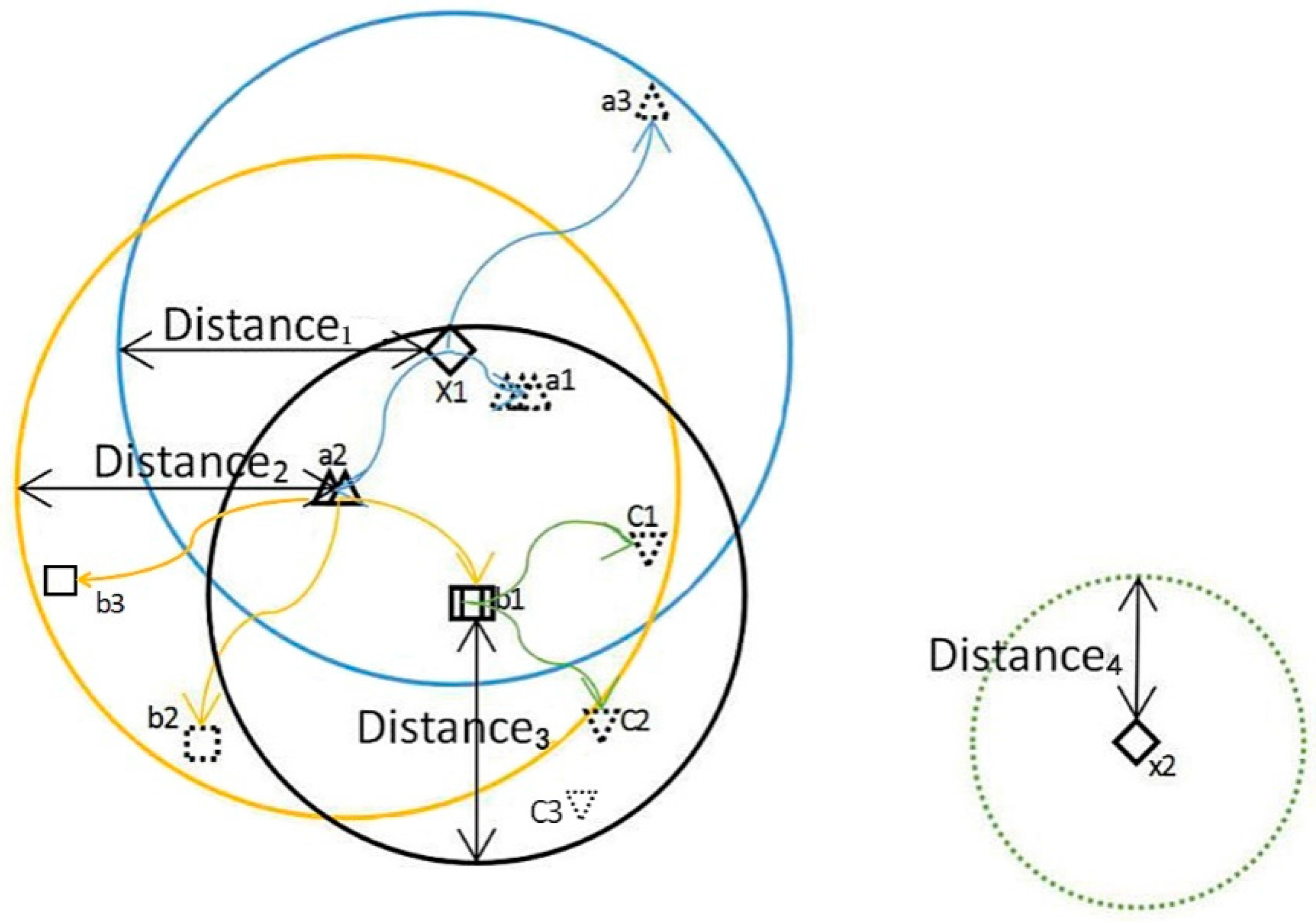
Figure 1 illustrates the process of migration and reproduction. The details are as follows:
- According to Rule 1, there was no such species in the region, due to sudden environmental changes or some kind of artificial action, original plants were spread over a random location in the region, as the ◇(x1) shows in Figure 1.
- The number of
![Applsci 08 00329 i002]() stand for the fitness. The higher the number, the higher the offspring’s fitness. It can be seen from the Figure 1 that if the offspring is closer to the original plant, the fitness is higher: fitness(a1) > fitness(a2) > fitness(a3). This matches Rule 5.
stand for the fitness. The higher the number, the higher the offspring’s fitness. It can be seen from the Figure 1 that if the offspring is closer to the original plant, the fitness is higher: fitness(a1) > fitness(a2) > fitness(a3). This matches Rule 5. - According to Rule 4, only some of the offspring plant survive because the fitness is different. As shown in Figure 1, the solid line indicates a living plant and the dotted line indicates that the plant is not living. Due to competition and other reasons, the offspring a1 with highest fitness did not survive, but a2 with the fitness less than a1 is alive and becomes a new original plant.
- Distance2and Distance3 are the propagation distance of
![Applsci 08 00329 i003]() (a2) and □(b1), respectively. According to Rule2, Distance2 evolves based on Distance1, and Distance3 is learning from Distance2 and Distance1. If b1 spreads seeds, the distance of b1’s offspring is based on Distance2 and Distance3.
(a2) and □(b1), respectively. According to Rule2, Distance2 evolves based on Distance1, and Distance3 is learning from Distance2 and Distance1. If b1 spreads seeds, the distance of b1’s offspring is based on Distance2 and Distance3. - Plants are constantly spreading seeds around and causing flora to migrate so that flora can find the best area to live.
- If all the offspring plants do not survive, as
![Applsci 08 00329 i004]() (c1,c2,c3) shown in Figure 1, a new original plant can be randomly generated in the region by allochory.
(c1,c2,c3) shown in Figure 1, a new original plant can be randomly generated in the region by allochory.


2.2.1. Evolution Behavior
The original plant spread seeds around in a circle with radius which is propagation distance. The propagation distance is evolved from the propagation distances of the parent plant and grandparent plant.
where d1j is the propagation distance of grandparent plant, d2j is the propagation distance of parent plant, c1 and c2 are the learning coefficient, and rand(0,1) denotes the independent uniformly distributed number in (0,1).
The new grandparent propagation distance is
The new parent propagation distance is the standard deviation between the positions of the original plant and offspring plant.
2.2.2. Spreading Behavior
First, the artificial flora algorithm randomly generated the original flora with N solutions, which is that there are N plants in the flora. The position of the original plants are expressed by the matrix Pi,j where i is the dimension and j is the number of plant in the flora.
where, d is the maximum limit area and rand(0,1) is an array of random numbers that are uniformly distributed between (0,1).
The position of the offspring plant is generated according to the propagation function as follows:
where, m is the number of seeds that one plant can propagate, stand for the position of offspring plant, Pi,j is the position of the original plant, and is a random number with the Gaussian distribution with mean 0 and variancedj. If no offspring plant survives, then a new original plant is generated according to Equation (4).
2.2.3. Select Behavior
Whether the offspring plants are alive is determined by survival probability as follows:
where is Qx to the power of (j × m − 1) and Qx is the selective probability. This value has to be between 0 and 1. It can be seen that the fitness of an offspring plant that is farther from the original plant is lower. Qx determines the exploration capability of the algorithm. Qx should be larger for the problem that is easy to get into local optimal solution. Fmax is maximum fitness in the flora this generation and is the fitness of j-th solution.
The fitness equation is an objective function. Then, a roulette wheel selection method is used to decide if the offspring plant is alive or not. The roulette wheel selection method is also called proportion select method [47]. Its basic purpose is to “accept according probability”; that is to say there are several alternatives and each has its own potential score. However, selection does not completely rely on the value of the score. Selection is according to the accepting probability. The higher the score, the greater the accepting probability is. Generate a random number r with a [0,1] uniform distribution every time, and offspring plant will be alive if the survival probability P is bigger than r, or it will die. Select N offspring plants among the alive offspring as new original plants and repeat the above behaviors until the accuracy requirement is reached or the maximum number of iterations is achieved.
2.3. The Proposed Algorithm Flow and Complexity Analysis
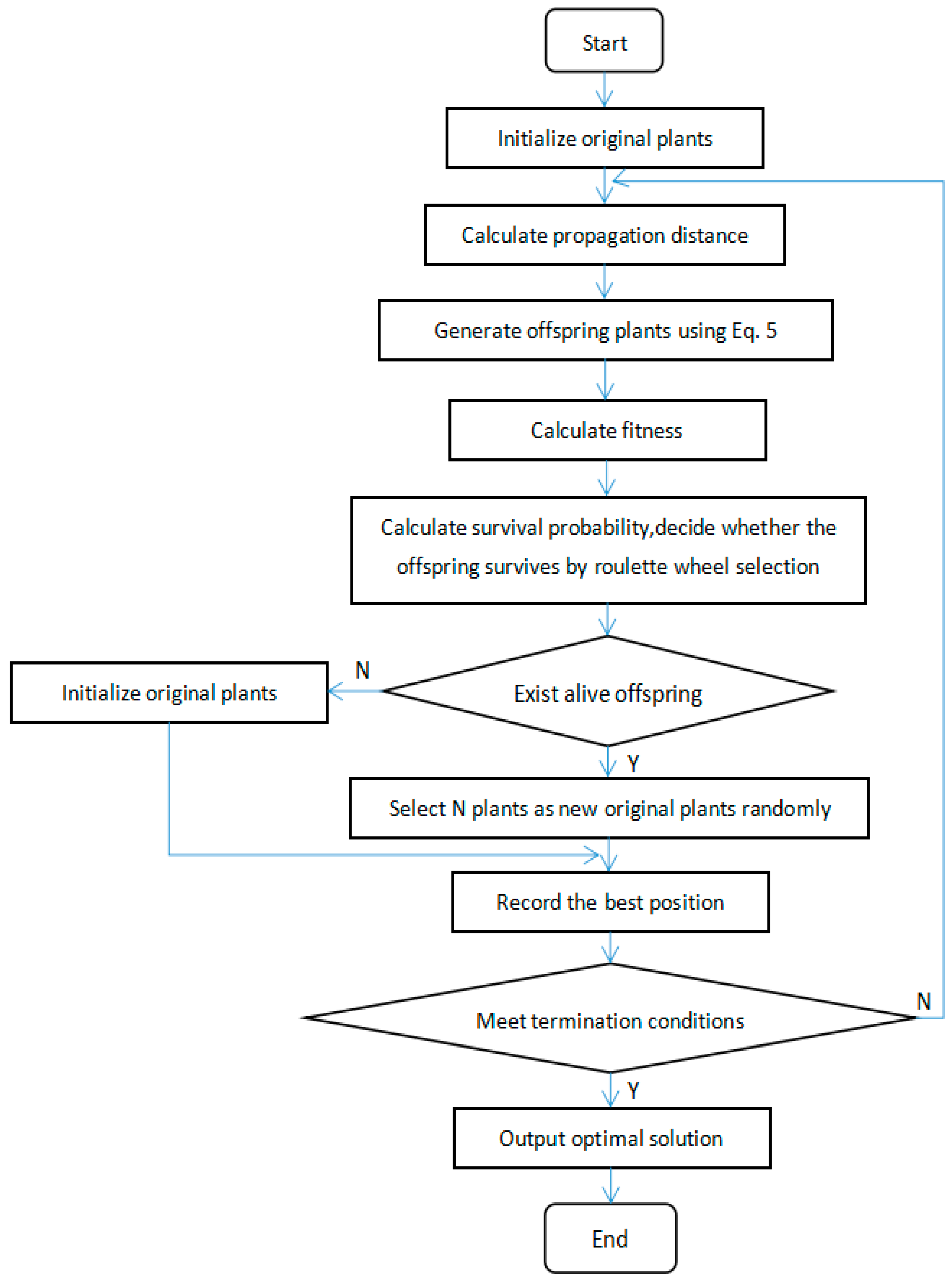
The basic flowchart of the proposed AF algorithm is shown in Figure 2. The main steps of artificial flora algorithm are as follows:
- (1)
- (Initialization according Equation (4), generate N original plants;
- (2)
- Calculate propagation distance according Equation (1), Equation (2) and Equation (3);
- (3)
- Generate offspring plants according Equation (5) and calculate their fitness;
- (4)
- Calculate the survival probability of offspring plants according to Equation (6)—whether the offspring survives or not is decided by the roulette wheel selection method;
- (5)
- If there are plants that survive, randomly select N plants as new original plants. If there are no surviving plant, generate new original plants according to Equation (4);
- (6)
- Record the best solution;
- (7)
- Estimate whether this meets the termination conditions. If so, output the optimal solution, otherwise goto step 2.
Based on the aforementioned descriptions, the AF algorithm can be summarized as the pseudo code shown in Table 1.
The time complexity of the algorithm can be measured by running time t(s) in order to facilitate the comparison of various algorithms.
where tA, tB, tP are the time required to perform every operation once and A(s), B(s), P(s) are the number of each operation.
In the artificial flora algorithm, the number of original plants is N, and the maximum branching number M is the number of seeds that one original plant can generate.t1 is the time to initialize population.t2is the time of calculating propagation distance.t3 is the time to update the plant position.t4 is the time to calculate the fitness.t5 is the time to calculate the survival probability.t6 is the time to decide which plant is alive this generation using roulette wheel selection method. The time complexity analysis of this algorithm is shown in Table 2. Therefore, we can see that the time complexity of artificial flora algorithm is O(NM) in Table 2.
3. Validation and Comparison
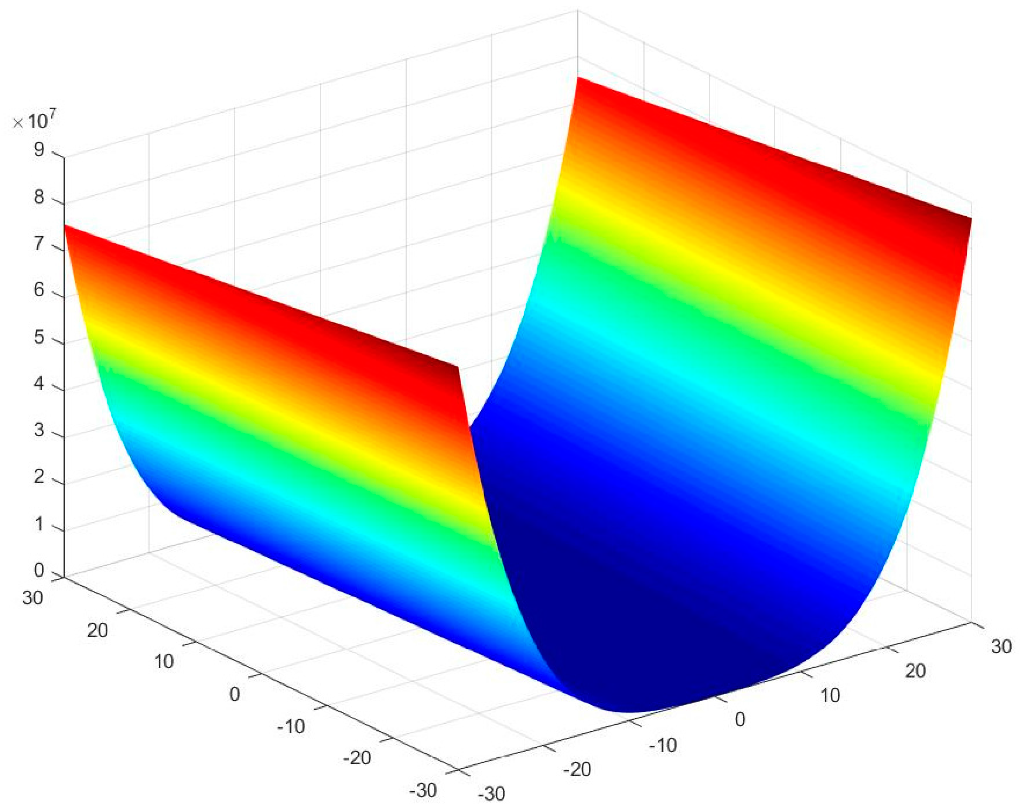
In this section, we use six benchmark functions [48,49] to test the efficiency and stability of artificial flora algorithm. The definition, bounds, and the optimum values of functions are shown in Table 3. For a two-dimensional condition, the value distributions of these functions are shown in Figure 3, Figure 4, Figure 5, Figure 6, Figure 7 and Figure 8. It can be seen from the Figure 3 and Figure 4 that Sphere (f1) and Rosenbrock (f2) functions are unimodal functions that can be used to test the optimization precision and performance of the algorithm. f3 to f6 functions are complex nonlinear multimodal functions. The general algorithm has difficulty finding the global optimal value. Because they have many local extreme points, they can be used to test the global search performance and the ability to avoid prematurity of algorithm.
The AF, PSO, and ABC are all bio-inspired swarm intelligence optimization algorithms. The PSO and ABC methods are widely used intelligent optimization algorithms. So, we compare the AF algorithm with the PSO [50] and ABC [36] algorithms to prove the advantages of this algorithm. The maximum number of iterations, cycle index, and the running environment are the same. The three algorithms will be iterated 1000 times respectively and run 50 times independently. All the experiments using MATLAB (2012a, MathWorks Company, Natick, MA, USA, 2012) are performed on a computer with Intel(R) Core(TM) i7-7700 CPU @ 3.60GHz and 8.00GB RAM running the Windows 10 operating system. The default parameters are shown in Table 4.
Table 5, Table 6 and Table 7 show the statistical results in 20-dimensional space, 50-dimensional space, and 100-dimensional space, respectively. According to the statistical results shown in Table 5, Table 6 and Table 7 , AF can find a more satisfactory solution with higher accuracy compare with PSO and ABC. For the unimodal function Sphere, AF can find the globally optimal solution. The accuracy of the solution obtained by AF is improved compare to those obtained by PSO and ABC. For Rosenbrock function, the accuracy of the solution is almost the same between AF and ABC in high dimensions (100-dimensional), and they are all better than PSO. However, the algorithm stability of AF is higher than that of ABC. For multimodal function (Rastrigin and Griewank), AF can steadily converge to the global optimal solution in 20-dimensional and 50-dimensional space, and in 100-dimensional space, AF can find the global optimal solution at best. For Schwefel function, the AF algorithm has better search precision in higher dimensions. In low dimensions, the search precision of the AF algorithm is superior to PSO but slightly worse than ABC. For Ackley function, AF is better than PSO and ABC for finding the global optimal solution.
On the whole, the solution accuracy obtained by the AF algorithm is improved obviously for the unimodal functions and the multimodal functions. It shows that the AF algorithm has strong exploration ability. Also, the stability of AF in these benchmark functions is better than that of PSO and ABC besides the Schwefel function.
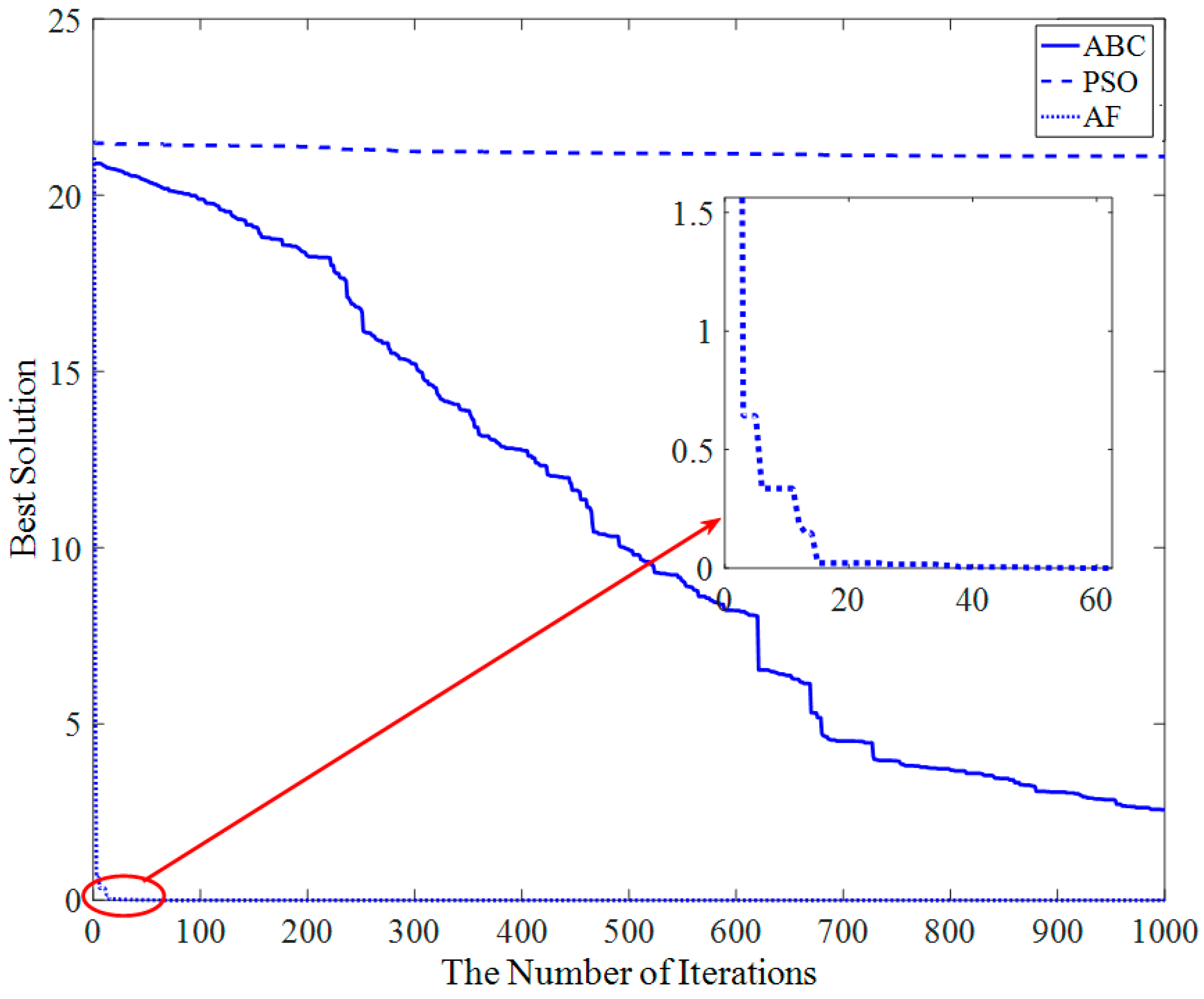
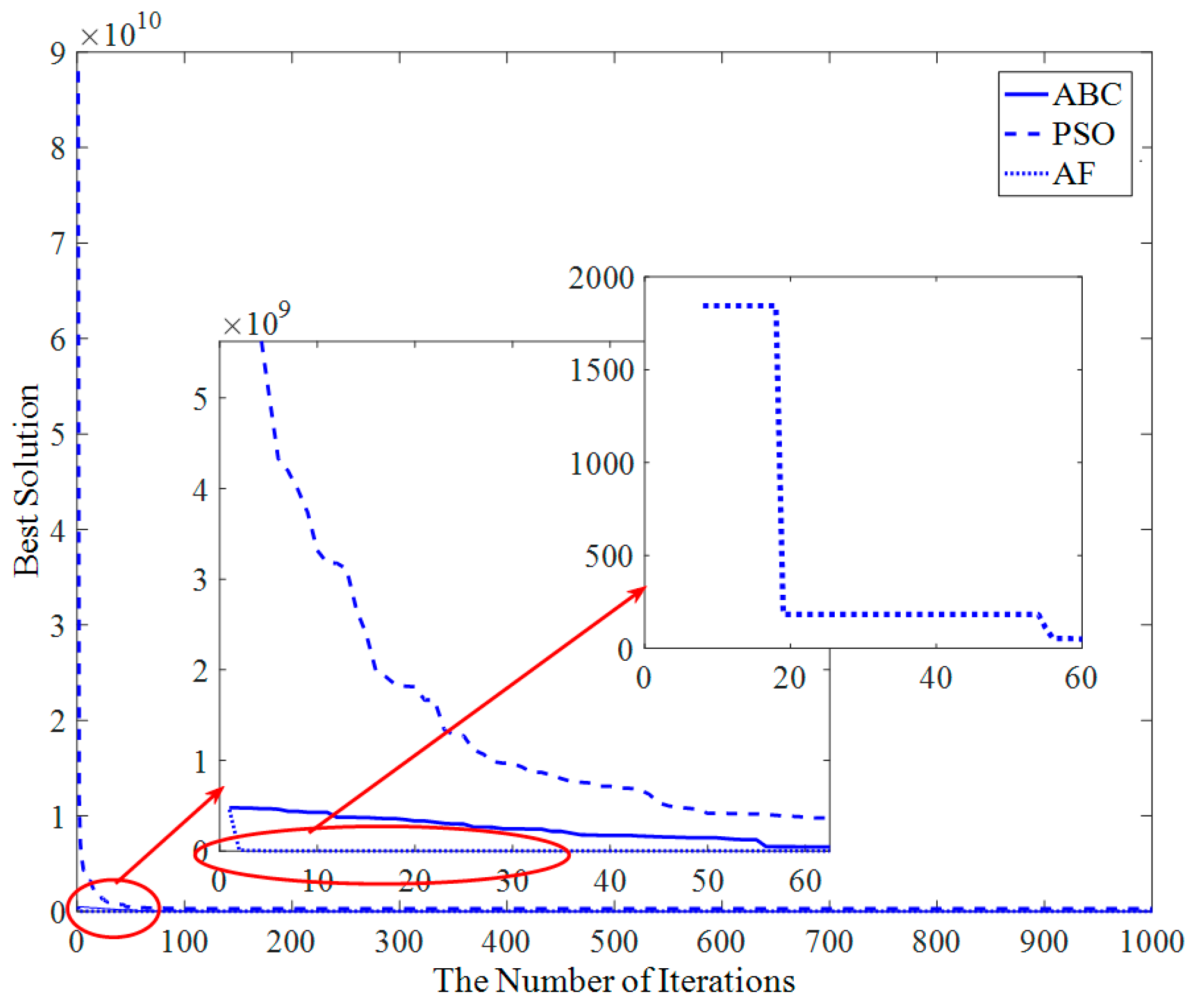
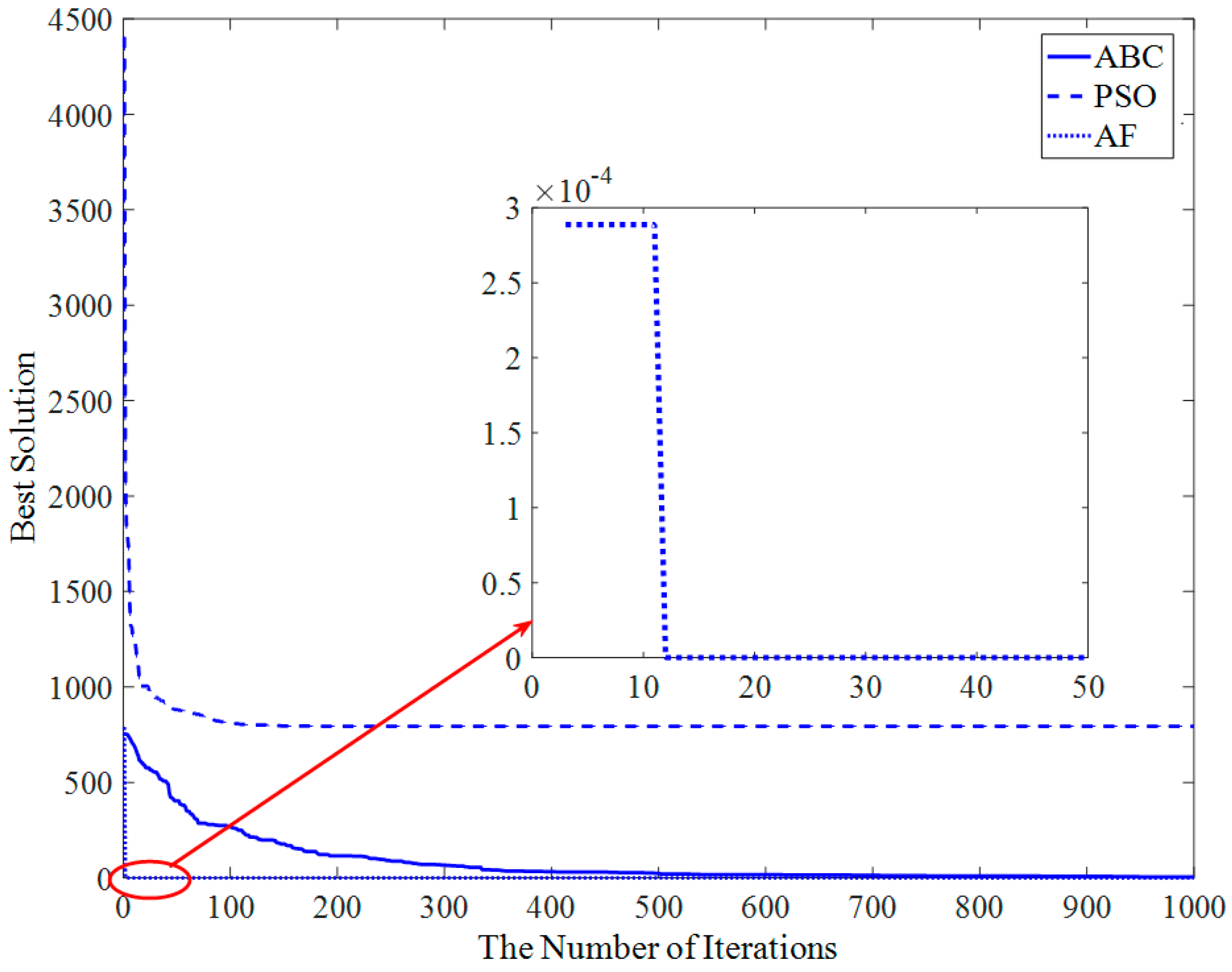
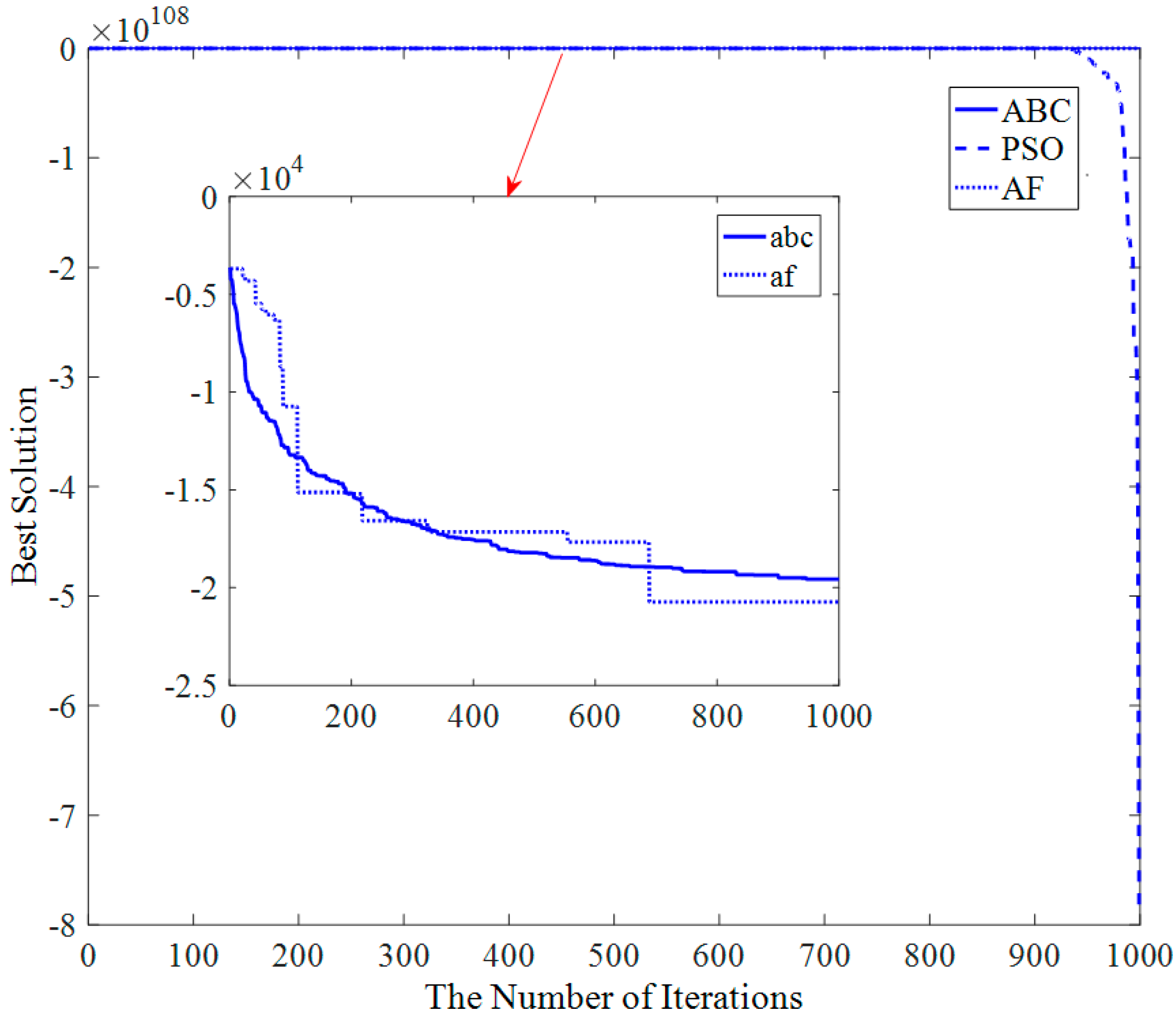
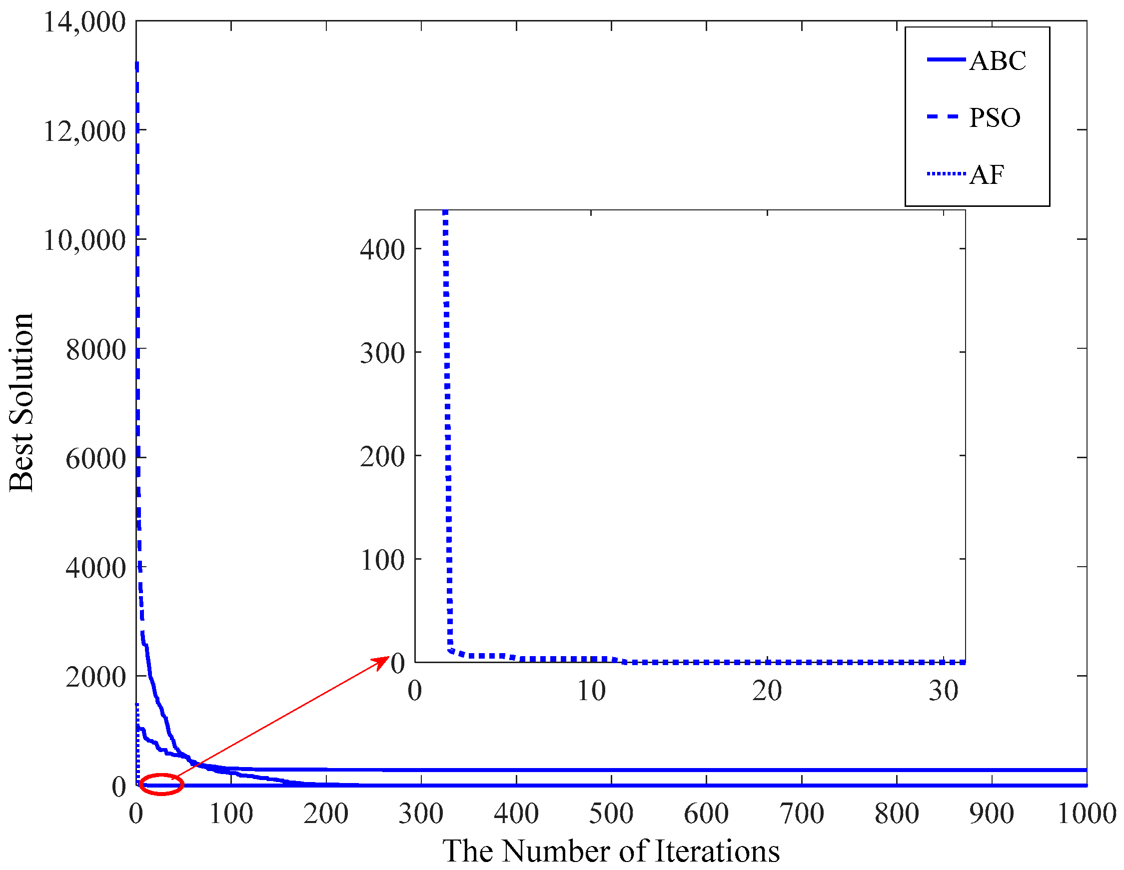
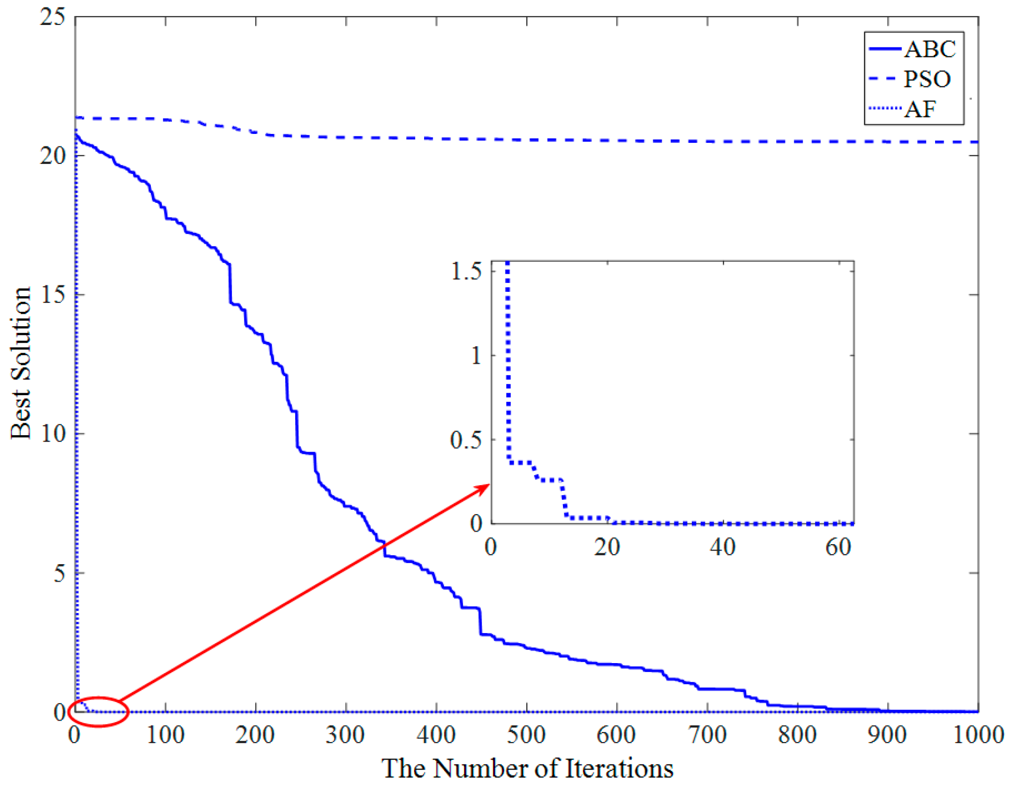
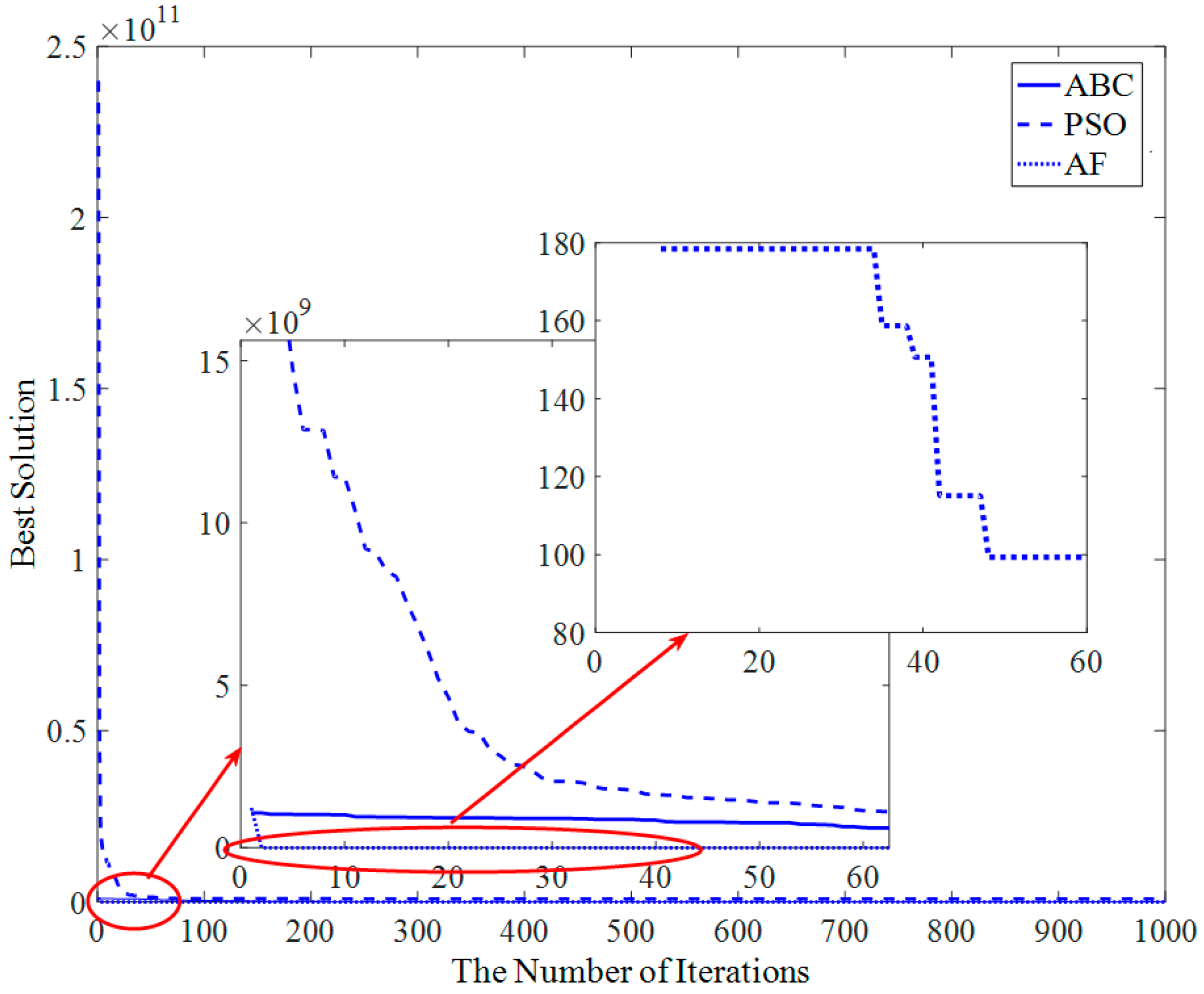
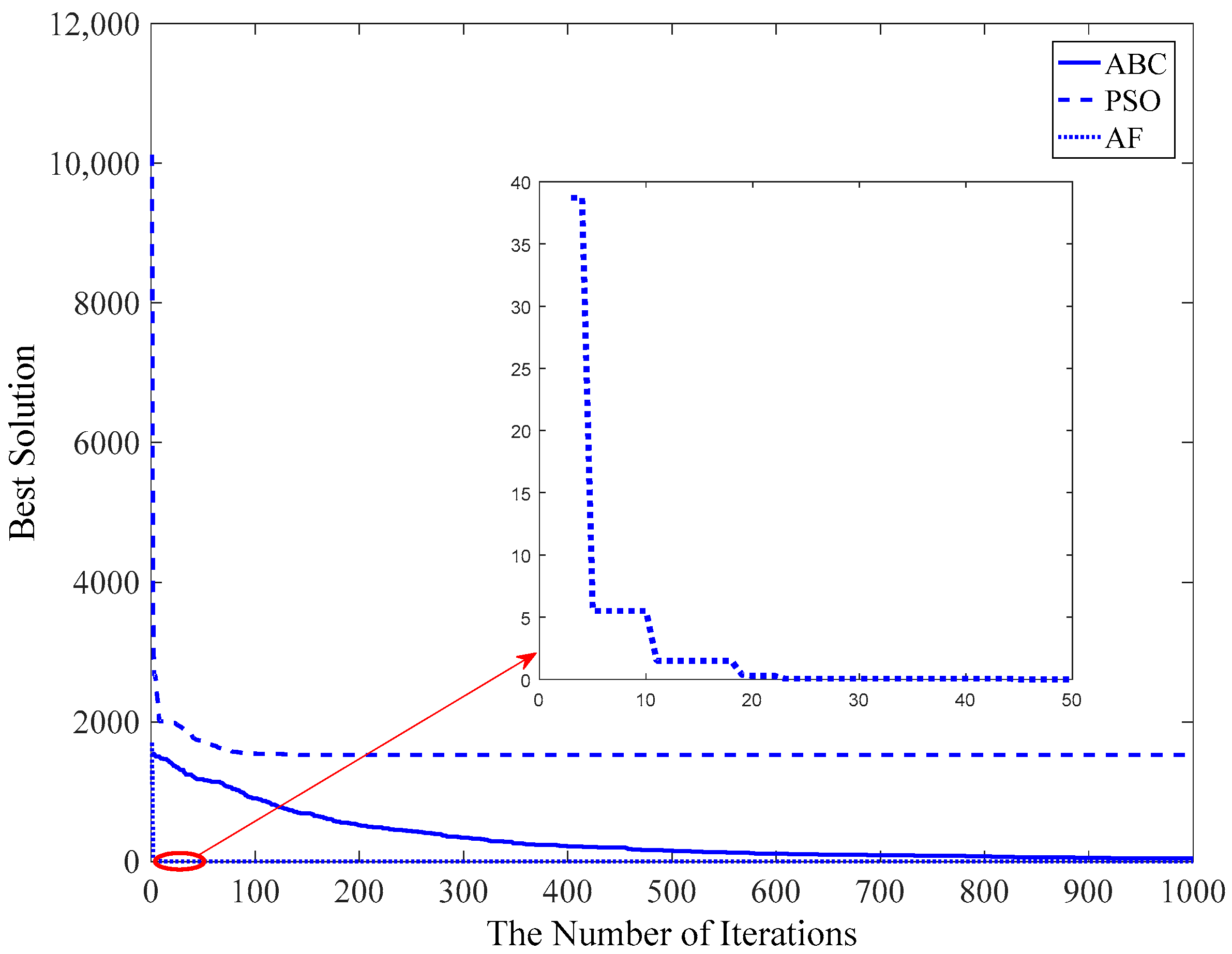
Figure 9, Figure 10, Figure 11, Figure 12, Figure 13 and Figure 14 show the convergence time of the three algorithms in 50-dimensional space, and Figure 15, Figure 16, Figure 17, Figure 18, Figure 19 and Figure 20 show the convergence time of the three algorithms in 100-dimensional space.
It can be seen from Figure 9 that the AF algorithm converges very quickly. The rate of convergence of ABC algorithm, PSO algorithm and AF algorithm is slowing down at 120th iteration, 50th iteration, and 15th iteration, respectively. The convergence curves of ABC and PSO intersect at the 50th iteration.
As shown in Figure 10, for Rosenbrock function, the PSO algorithm and ABC algorithm both converge at about 100 iterations, and the AF algorithm converges at about the 55th iteration.
Figure 11 illustrates that the convergence rate of the AF algorithm is still better than the other two algorithms for Rastrig in function. The AF algorithm is convergent to a good numerical solution at the 15th iteration. The PSO algorithm converges fast, but it is easily trapped into the local optimal solution. The convergence rate of ABC is slow.
Schwefel is a typical deceptive function, as shown in Figure 12. The convergence rate of the AF algorithm is similar to that of ABC for Schwefel function.
Figure 13 shows that the AF algorithm converges at about the 23rd iteration, and the PSO and ABC algorithms converge at about the 50th iteration and 200th iteration, respectively.
As Figure 14 shows, for Ackley function, the PSO algorithm is easily trapped into a local optimization. The convergence speed of the ABC algorithm is slow. The ABC algorithm converges at about the 900th iteration. However, the AF algorithm can get a convergence solution at only the 40th iteration.
It can be seen from Figure 15Figure 16, Figure 17, Figure 18, Figure 19 and Figure 20 that the trend of convergence curves in 100-dimensional space is similar to that in 50-dimensional space.
It can be concluded that the AF algorithm can get a solution with higher accuracy and stability than PSO and ABC according to Table 5, Table 6 and Table 7 and Figure 9, Figure 10, Figure 11, Figure 12, Figure 13, Figure 14, Figure 15, Figure 16, Figure 17, Figure 18, Figure 19 and Figure 20. First, since the AF algorithm selects the alive offspring plants as new original plants at each iteration, it can take the local optimal position as the center to explore the surrounding space. It can converge to the optimal point rapidly. Second, original plants can spread seeds to any direction and distance within the propagation range. It guarantees the local search capability of the algorithm. Third, when there is no better offspring plant, in order to explore the possibility that a better solution exists, new original plants will be generated randomly in the function domain. This can help the AF algorithm to skip the local optimum and improve the performance of global searching. Therefore, the AF algorithm has excellent accuracy, stability, and effectiveness.
4. Conclusions
The beautiful posture of birds and the perfect cooperation of a bee colony left an impression on people’s minds, so the PSO algorithm and ABC algorithm were proposed. In this paper, the proposed artificial flora algorithm is inspired by the migration and reproduction behavior of flora. There are three main behaviors, including evolution behavior, spreading behavior, and select behavior. In evolution behavior, the propagation distance of offspring plants is evolution based on the propagation distance of parent plant and grandparent plant. The propagation distance is optimized in each generation. Since the propagation distance of offspring plants is not a complete inheritance to the parent plant, there is an opportunity for the algorithm to get out of the local optimal solution. Spreading behavior includes autochory and allochory. Autochory provides the opportunity for the original plant to explore the optimal location around itself. This behavior provides local search capability to the algorithm. Allochory provides opportunity for original plant to explore greater space, and global search capability of the algorithm is obtained from this behavior. According to the natural law of survival of the fittest, the greater the survival probability of a plant with higher fitness, and thus the natural law is called select behavior.
Several simulations have shown the effective performance of the proposed algorithm when compared with PSO and ABC algorithms. The AF algorithm improves the algorithm's ability to find the global optimal solution and accuracy and also speeds up the convergence speed.
In the future, we focus on solving discrete, multi-objective, combinatorial, and more complex problems using the AF algorithm and its variants. For example, we are now trying to apply AF to multi-objective optimization problems. Using the method of generating a mesh, AF can converge to the optimal Pareto front. In addition, a lot of practical problems can be converted to optimization problems, and then we can use AF to find a satisfactory solution. For instance, AF can be used to find a satisfactory solution and can applied to parameter optimization and cluster analysis.
Acknowledgments
This work was supported by the National Natural Science Foundation of China under Grant No. 61403068; Natural Science Foundation of Hebei Province under Grant No. F2015501097 and No. F2016501080; Fundamental Research Funds for the Central Universities of China under Grant No. N130323002, No. N130323004 and N152302001.
Author Contributions
Long Cheng and Xue-han Wu conceived and designed the experiments; Yan Wang performed the experiments; Xue-han Wu and Yan Wang analyzed the data; Long Cheng contributed analysis tools; Long Cheng and Xue-han Wu wrote the paper.
Conflicts of Interest
The authors declare that there is no conflict of interests regarding the publication of this paper.
References
- Cao, Z.; Wang, L. An effective cooperative coevolution framework integrating global and local search for large scale optimization problems. In Proceedings of the 2015 IEEE Congress on Evolutionary Computation, Sendai, Japan, 25–28 May 2015; pp. 1986–1993. [Google Scholar]
- Battiti, R. First- and Second-Order Methods for Learning: Between Steepest Descent and Newton’s Method; MIT Press: Cambridge, MA, USA, 1992. [Google Scholar]
- Liang, X.B.; Wang, J. A recurrent neural network for nonlinear optimization with a continuously differentiable objective function and bound constraints. IEEE Trans. Neural Netw. 2000, 11, 1251–1262. [Google Scholar] [PubMed]
- Li, J.; Fong, S.; Wong, R. Adaptive multi-objective swarm fusion for imbalanced data classification. Inf. Fusion 2018, 39, 1–24. [Google Scholar] [CrossRef]
- Han, G.; Liu, L.; Chan, S.; Yu, R.; Yang, Y. HySense: A Hybrid Mobile CrowdSensing Framework for Sensing Opportunities Compensation under Dynamic Coverage Constraint. IEEE Commun. Mag. 2017, 55, 93–99. [Google Scholar] [CrossRef]
- Navalertporn, T.; Afzulpurkar, N.V. Optimization of tile manufacturing process using particle swarm optimization. Swarm Evol. Comput. 2011, 1, 97–109. [Google Scholar] [CrossRef]
- Pan, Q.; Tasgetiren, M.; Suganthan, P. A discrete artificial bee colony algorithm for the lot-streaming flow shop scheduling problem. Inf. Sci. 2011, 181, 2455–2468. [Google Scholar] [CrossRef]
- Duan, H.; Luo, Q. New progresses in swarm intelligence-based computation. Int. J. Bio-Inspired Comput. 2015, 7, 26–35. [Google Scholar] [CrossRef]
- Tang, Q.; Shen, Y.; Hu, C. Swarm Intelligence: Based Cooperation Optimization of Multi-Modal Functions. Cogn. Comput. 2013, 5, 48–55. [Google Scholar] [CrossRef]
- Demertzis, K.; Iliadis, L. Adaptive elitist differential evolution extreme learning machines on big data: Intelligent recognition of invasive species. In Advances in Big Data; Springer International Publishing: Berlin/Heidelberg, Germany, 2016. [Google Scholar]
- Du, X.P.; Cheng, L.; Liu, L. A Swarm Intelligence Algorithm for Joint Sparse Recovery. IEEE Signal Process. Lett. 2013, 20, 611–614. [Google Scholar]
- Zaman, F.; Qureshi, I.M.; Munir, F. Four-dimensional parameter estimation of plane waves using swarming intelligence. Chin. Phys. B 2014, 23, 078402. [Google Scholar] [CrossRef]
- Jain, C.; Verma, H.K.; Arya, L.D. A novel statistically tracked particle swarm optimization method for automatic generation control. J. Mod. Power Syst. Clean Energy 2014, 2, 396–410. [Google Scholar] [CrossRef]
- Torabi, A.J.; Er, M.J.; Li, X. A Survey on Artificial Intelligence-Based Modeling Techniques for High Speed Milling Processes. IEEE Syst. J. 2015, 9, 1069–1080. [Google Scholar] [CrossRef]
- Nebti, S.; Boukerram, A. Swarm intelligence inspired classifiers for facial recognition. Swarm Evol. Comput. 2017, 32, 150–166. [Google Scholar] [CrossRef]
- Teodorovic, D. Swarm intelligence systems for transportation engineering: Principles and applications. Transp. Res. Part C-Emerg. Technol. 2008, 16, 651–667. [Google Scholar] [CrossRef]
- Drechsler, R.; Gockel, N. Genetic algorithm for data sequencing. Electron. Lett. 1997, 33, 843–845. [Google Scholar] [CrossRef]
- Jong, E.D.; Watson, R.A.; Pollack, J.B. Reducing Bloat and Promoting Diversity using Multi-Objective Methods. In Proceedings of the Genetic and Evolutionary Computation Conference, San Francisco, CA, USA, 7–11 July 2001; pp. 1–8. [Google Scholar]
- Pornsing, C.; Sodhi, M.S.; Lamond, B.F. Novel self-adaptive particle swarm optimization methods. Soft Comput. 2016, 20, 3579–3593. [Google Scholar] [CrossRef]
- Karaboga, D.; Gorkemli, B. A quick artificial bee colony (qABC) algorithm and its performance on optimization problems. Appl. Soft Comput. 2014, 23, 227–238. [Google Scholar] [CrossRef]
- Luh, G.C.; Lin, C.Y. Structural topology optimization using ant colony optimization algorithm. Appl. Soft Comput. 2009, 9, 1343–1353. [Google Scholar] [CrossRef]
- Wang, H.B.; Fan, C.C.; Tu, X.Y. AFSAOCP: A novel artificial fish swarm optimization algorithm aided by ocean current power. Appl. Intell. 2016, 45, 992–1007. [Google Scholar] [CrossRef]
- Wang, H.; Wang, W.; Zhou, X. Firefly algorithm with neighborhood attraction. Inf. Sci. 2017, 382, 374–387. [Google Scholar] [CrossRef]
- Gandomi, A.H.; Talatahari, S.; Tadbiri, F. Krill herd algorithm for optimum design of truss structures. Int. J. Bio-Inspired Comput. 2013, 5, 281–288. [Google Scholar] [CrossRef]
- Yang, X.S. Flower Pollination Algorithm for Global Optimization. In Proceedings of the 11th International Conference on Unconventional Computation and Natural Computation, Orléans, France, 3–7 September 2012; Springer: Berlin/Heidelberg, Germany, 2012; pp. 240–249. [Google Scholar]
- Holland, J.H. Adaptation in Natural and Artificial Systems; MIT Press: Cambridge, MA, USA, 1992. [Google Scholar]
- Dick, G.; Whigham, P. The behaviour of genetic drift in a spatially-structured evolutionary algorithm. In Proceedings of the IEEE Congress on Evolutionary Computation, Edinburgh, UK, 2–5 September 2005; Volume 2, pp. 1855–1860. [Google Scholar]
- Ashlock, D.; Smucker, M.; Walker, J. Graph based genetic algorithms. In Proceedings of the Congress on Evolutionary Computation, Washington, DC, USA, 6–9 July 1999; Volume 2, p. 1368. [Google Scholar]
- Gasparri, A. A Spatially Structured Genetic Algorithm over Complex Networks for Mobile Robot Localisation. In Proceedings of the IEEE International Conference on Robotics and Automation, Roma, Italy, 10–14 April 2007; pp. 4277–4282. [Google Scholar]
- Srinivas, M.; Patnaik, L.M. Adaptive probabilities of crossover and mutation in genetic algorithms. IEEE Trans. Syst. Man Cybern. 2002, 24, 656–667. [Google Scholar] [CrossRef]
- Kennedy, J.; Eberhart, R. Particle swarm optimization. In Proceedings of the IEEE International Conference on Neural Networks, Perth, Australia, 27 November–1 December 1995; IEEE: Middlesex County, NJ, USA, 1995; Volume 4, pp. 1942–1948. [Google Scholar]
- Clerc, M.; Kennedy, J. The particle swarm—Explosion, stability, and convergence in a multidimensional complex space. IEEE Trans. Evol. Comput. 2002, 6, 58–73. [Google Scholar] [CrossRef]
- Suganthan, P. Particle swarm optimizer with neighborhood operator. In Proceedings of the IEEE Congress on Evolutionary Computation, Washington, DC, USA, 6–9 July 1999; pp. 1958–1961. [Google Scholar]
- Parsopoulos, K.E.; Vrahatis, M.N. On the computation of all global minimizers through particle swarm optimization. IEEE Trans. Evol. Comput. 2004, 8, 211–224. [Google Scholar] [CrossRef]
- Voss, M.S. Principal Component Particle Swarm Optimization (PCPSO). In Proceedings of the IEEE Swarm Intelligence Symposium, Pasadena, CA, USA, 8–10 June 2005; pp. 401–404. [Google Scholar]
- Karaboga, D. An Idea Based on Honey Bee Swarm for Numerical Optimization; Erciyes University: Kayseri, Turkey, 2005. [Google Scholar]
- Alam, M.S.; Kabir, M.W.U.; Islam, M.M. Self-adaptation of mutation step size in Artificial Bee Colony algorithm for continuous function optimization. In Proceedings of the 2013 IEEE International Conference on Computer and Information Technology, Dhaka, Bangladesh, 23–25 December 2011; IEEE: Middlesex County, NJ, USA, 2011; pp. 69–74. [Google Scholar]
- Zhang, D.; Guan, X.; Tang, Y. Modified Artificial Bee Colony Algorithms for Numerical Optimization. In Proceedings of the 2011 3rd International Workshop on Intelligent Systems and Applications, Wuhan, China, 28–29 May 2011; pp. 1–4. [Google Scholar]
- Zhong, F.; Li, H.; Zhong, S. A modified ABC algorithm based on improved-global-best-guided approach and adaptive-limit strategy for global optimization. Appl. Soft Comput. 2016, 46, 469–486. [Google Scholar] [CrossRef]
- Rajasekhar, A.; Abraham, A.; Pant, M. Levy mutated Artificial Bee Colony algorithm for global optimization. In Proceedings of the 2011 IEEE International Conference on Systems, Man, and Cybernetics, Anchorage, AK, USA, 9–12 October 2011; pp. 655–662. [Google Scholar]
- Pagie, L.; Mitchell, M. A comparison of evolutionary and coevolutionary search. Int. J. Comput. Intell. Appl. 2002, 2, 53–69. [Google Scholar] [CrossRef]
- Wiegand, R.P.; Sarma, J. Spatial Embedding and Loss of Gradient in Cooperative Coevolutionary Algorithms. In Proceedings of the International Conference on Parallel Problem Solving from Nature, Berlin, Germany, 22–26 September 1996; Springer: Berlin/Heidelberg, Germany, 2004; pp. 912–921. [Google Scholar]
- Rosin, C.D.; Belew, R.K. Methods for Competitive Co-Evolution: Finding Opponents Worth Beating. In Proceedings of the International Conference on Genetic Algorithms, Pittsburgh, PA, USA, 15–19 June 1995; pp. 373–381. [Google Scholar]
- Cartlidge, J.P.; Bulloc, S.G. Combating coevolutionary disengagement by reducing parasite virulence. Evol. Comput. 2004, 12, 193–222. [Google Scholar] [CrossRef] [PubMed] [Green Version]
- Williams, N.; Mitchell, M. Investigating the success of spatial coevolution. In Proceedings of the 7th Annual Conference on Genetic And Evolutionary Computation, Washington, DC, USA, 25–29 June 2005; pp. 523–530. [Google Scholar]
- Hillis, W.D. Co-evolving Parasites Improve Simulated Evolution as an Optimization Procedure. Phys. D Nonlinear Phenom. 1990, 42, 228–234. [Google Scholar] [CrossRef]
- Ling, S.H.; Leung, F.H.F. An Improved Genetic Algorithm with Average-bound Crossover and Wavelet Mutation Operations. Soft Comput. 2007, 11, 7–31. [Google Scholar] [CrossRef]
- Akay, B.; Karaboga, D. A modified Artificial Bee Colony algorithm for real-parameter optimization. Inf. Sci. 2012, 192, 120–142. [Google Scholar] [CrossRef]
- Meng, X.B.; Gao, X.Z.; Lu, L. A new bio-inspired optimisation algorithm: Bird Swarm Algorithm. J. Exp. Theor. Artif. Intell. 2016, 38, 673–687. [Google Scholar] [CrossRef]
- Shi, Y.; Eberhart, R. A modified particle swarm optimizer. In Proceedings of the 1998 IEEE International Conference on Evolutionary Computation Proceedings, Anchorage, AK, USA, 4–9 May 1998; pp. 69–73. [Google Scholar]
Figure 1.
The process of migration and reproduction.

Figure 2.
Algorithm flow of artificial flora algorithm.

Figure 3.
Three-dimensional image of Sphere function (f1).
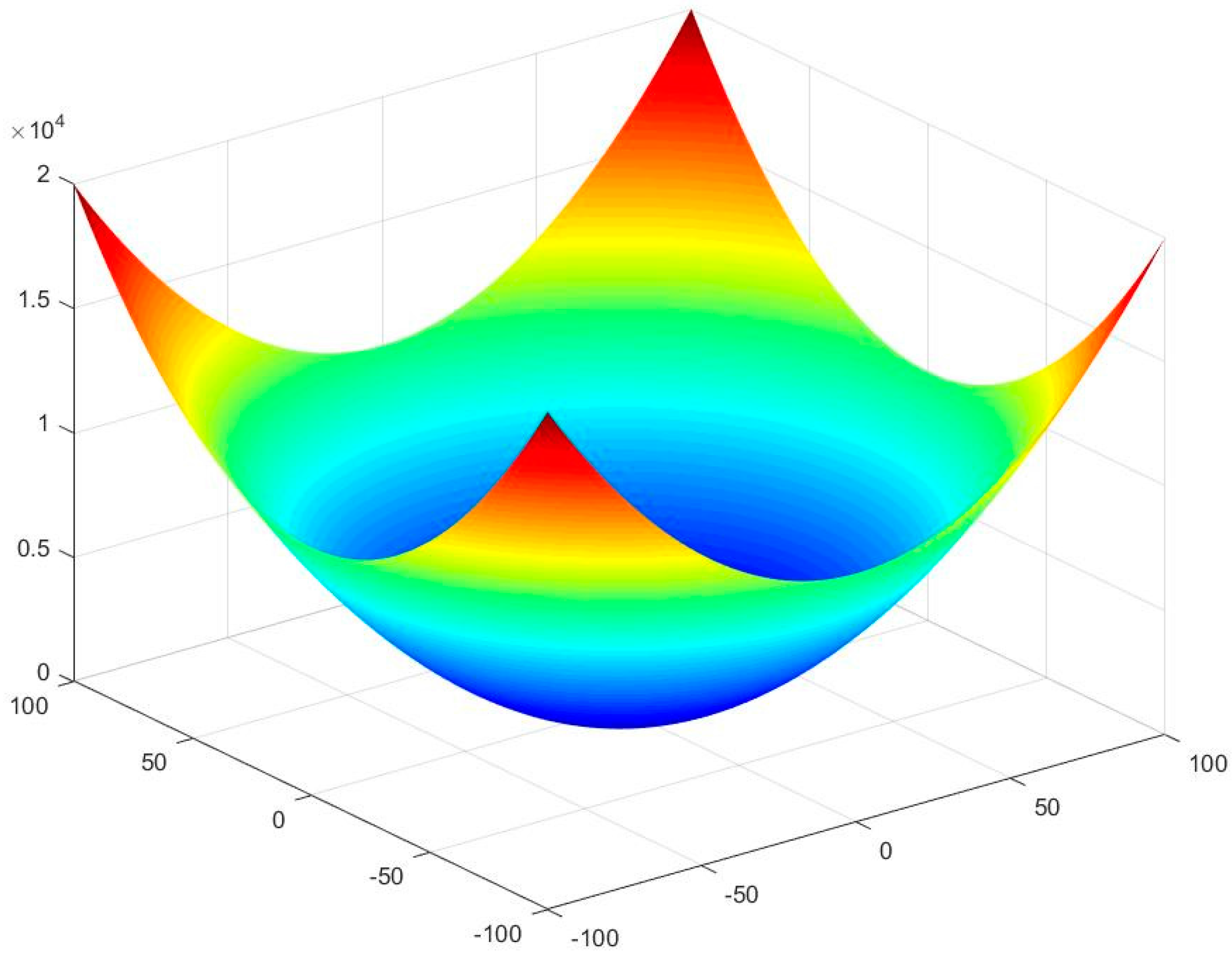
Figure 4.
Three-dimensional image of Rosenbrock function (f2).

Figure 5.
Three-dimensional image of Rastrigin function (f3).
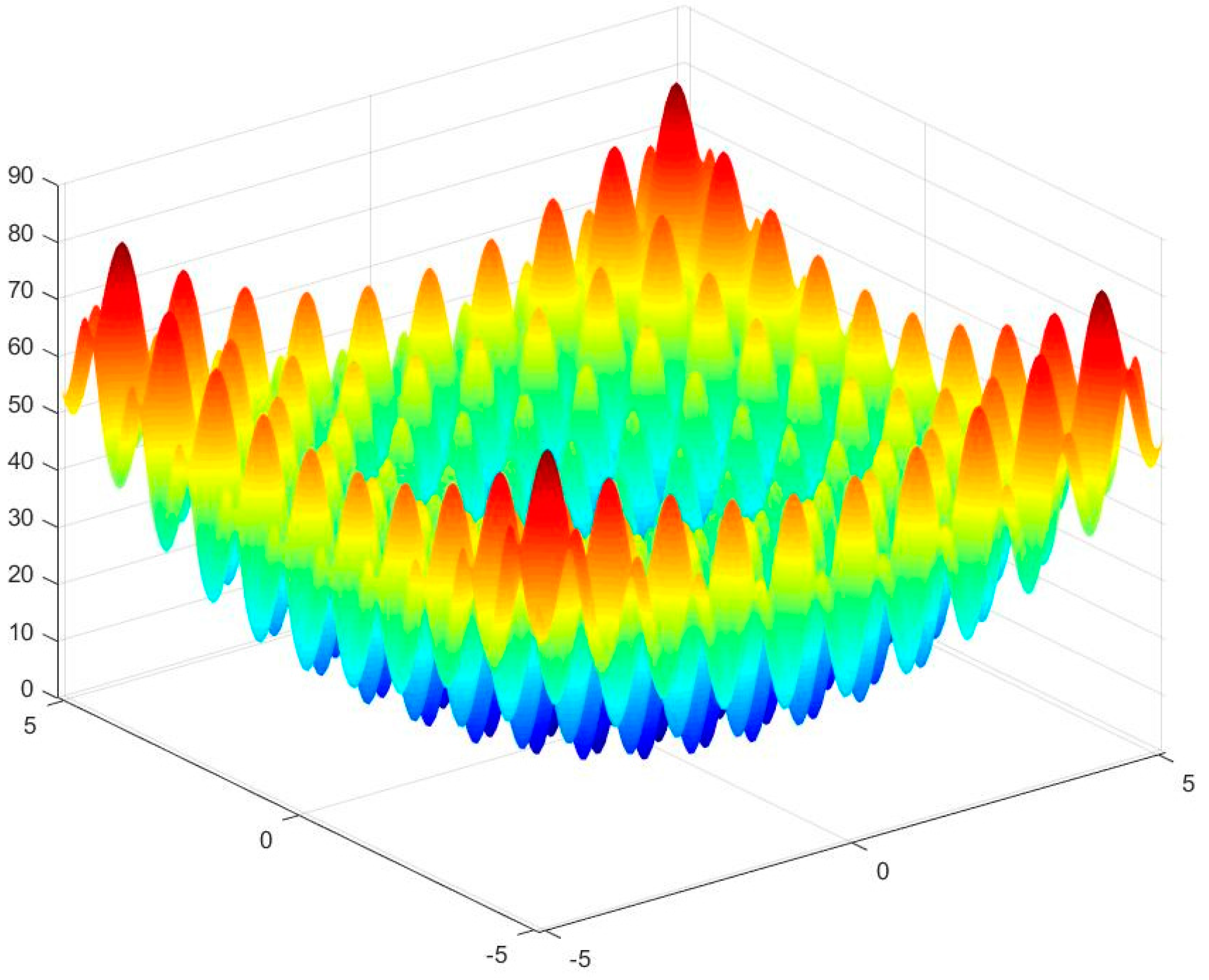
Figure 6.
Three-dimensional image of Schwefel function (f4).
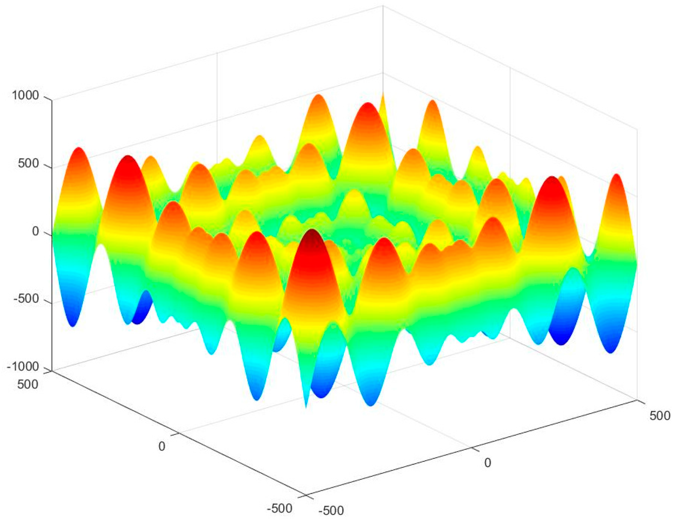
Figure 7.
Three-dimensional image of Griewank function (f5).
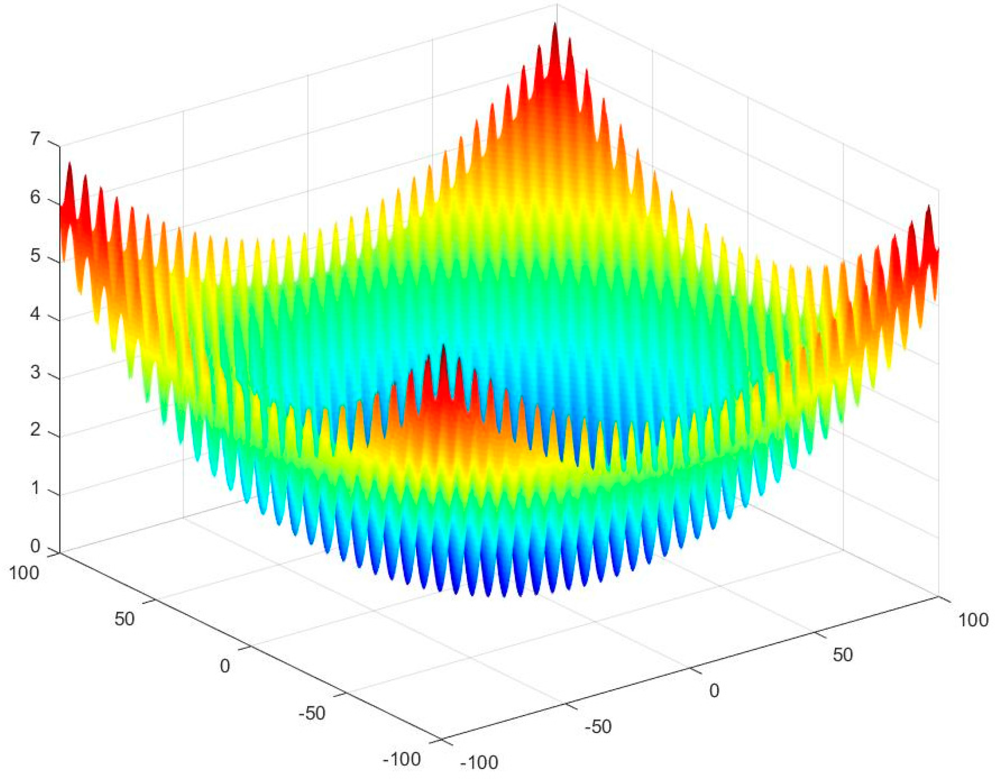
Figure 8.
Three-dimensional image of Ackley function (f6).
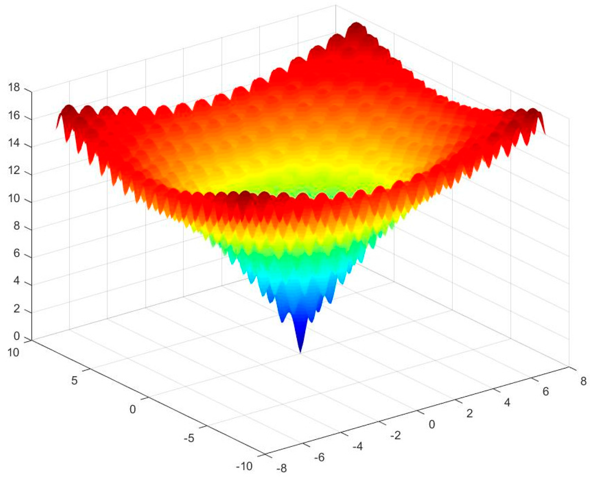
Figure 9.
The convergence curve of the three algorithms for Sphere function in 50-dimensional space. PSO: particle swarm optimization algorithm; ABC: artificial bee colony algorithm; AF: artificial flora algorithm.
Figure 9.
The convergence curve of the three algorithms for Sphere function in 50-dimensional space. PSO: particle swarm optimization algorithm; ABC: artificial bee colony algorithm; AF: artificial flora algorithm.
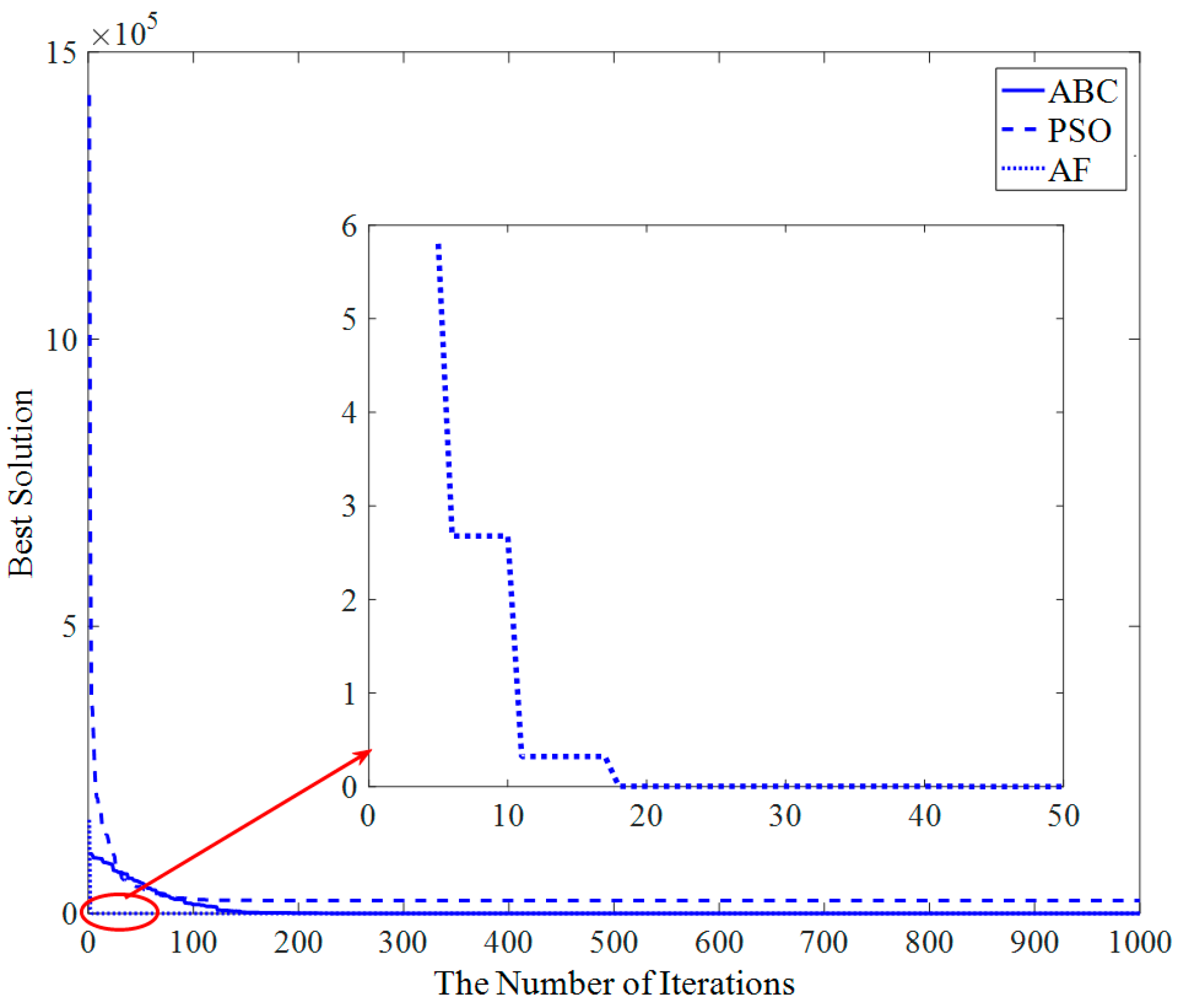
Figure 10.
The convergence curve of the three algorithms for Rosenbrock function in 50-dimensional space.
Figure 10.
The convergence curve of the three algorithms for Rosenbrock function in 50-dimensional space.

Figure 11.
The convergence curve of the three algorithms for Rastrigin function in 50-dimensional space.
Figure 11.
The convergence curve of the three algorithms for Rastrigin function in 50-dimensional space.

Figure 12.
The convergence curve of the three algorithms for Schwefel function in 50-dimensional space.
Figure 12.
The convergence curve of the three algorithms for Schwefel function in 50-dimensional space.

Figure 13.
The convergence curve of the three algorithms for Griewank function in 50-dimensional space.
Figure 13.
The convergence curve of the three algorithms for Griewank function in 50-dimensional space.

Figure 14.
The convergence curve of the three algorithms for Ackley function in 50-dimensional space.
Figure 14.
The convergence curve of the three algorithms for Ackley function in 50-dimensional space.

Figure 15.
The convergence curve of the three algorithms for Sphere function in 100-dimensional space.
Figure 15.
The convergence curve of the three algorithms for Sphere function in 100-dimensional space.
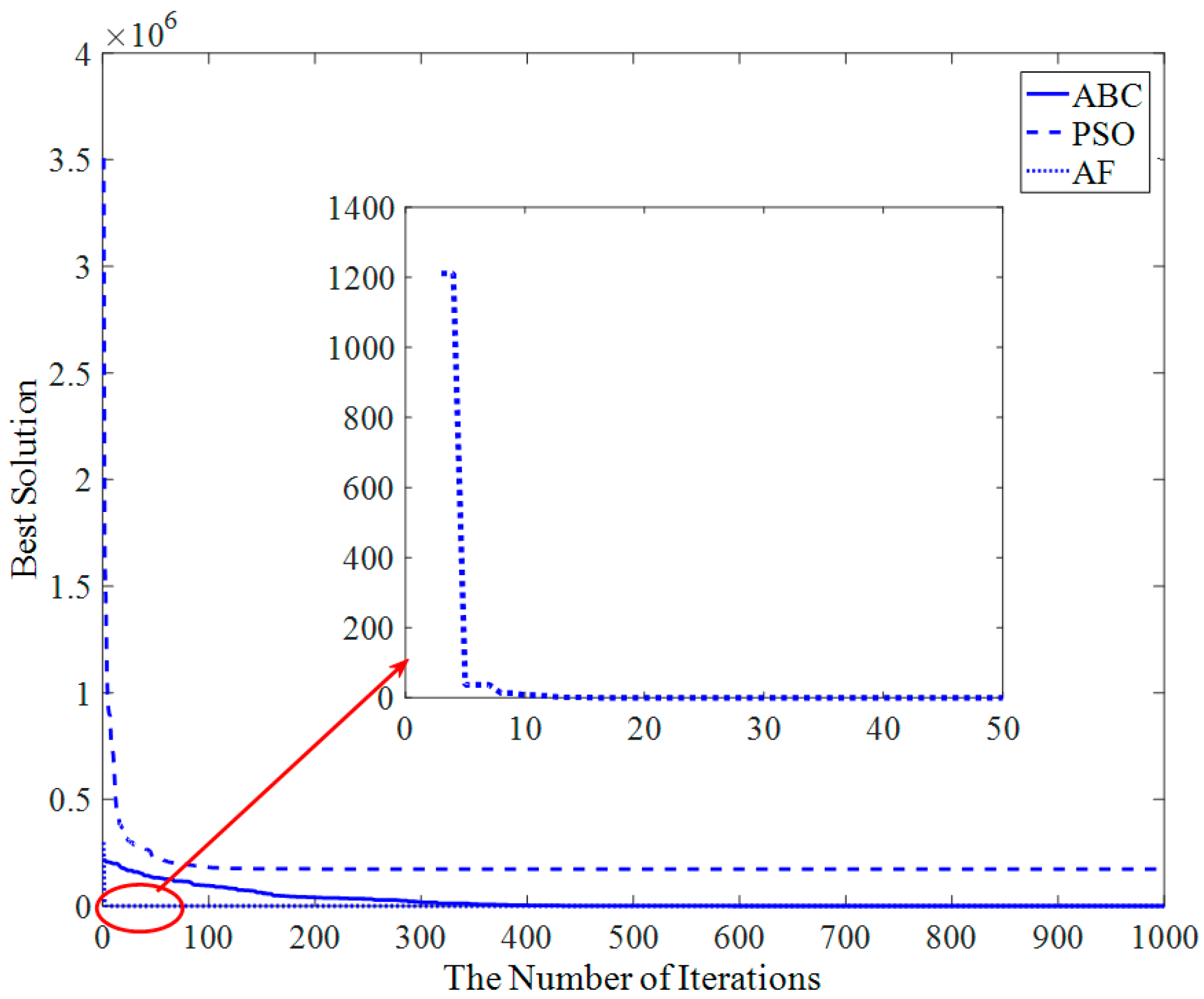
Figure 16.
The convergence curve of the three algorithms for Rosenbrock function in 100-dimensional space.
Figure 16.
The convergence curve of the three algorithms for Rosenbrock function in 100-dimensional space.

Figure 17.
The convergence curve of the three algorithms for Rastrigin function in 100-dimensional space.
Figure 17.
The convergence curve of the three algorithms for Rastrigin function in 100-dimensional space.

Figure 18.
The convergence curve of the three algorithms for Schwefel function in 100-dimensional space.
Figure 18.
The convergence curve of the three algorithms for Schwefel function in 100-dimensional space.
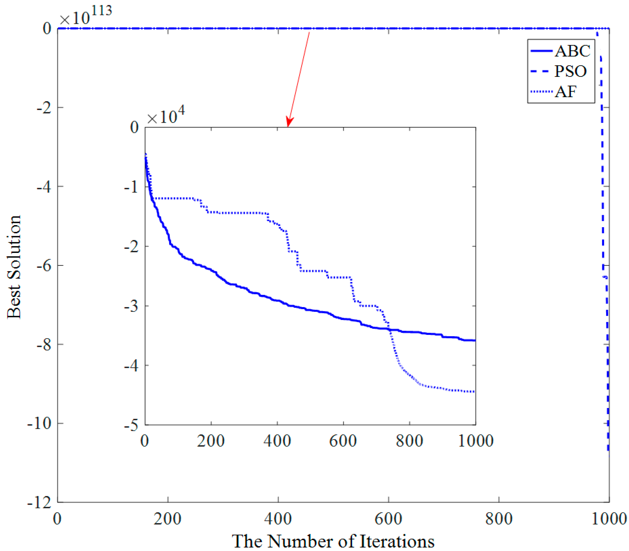
Figure 19.
The convergence curve of the three algorithms for Griewank function in 100-dimensional space.
Figure 19.
The convergence curve of the three algorithms for Griewank function in 100-dimensional space.
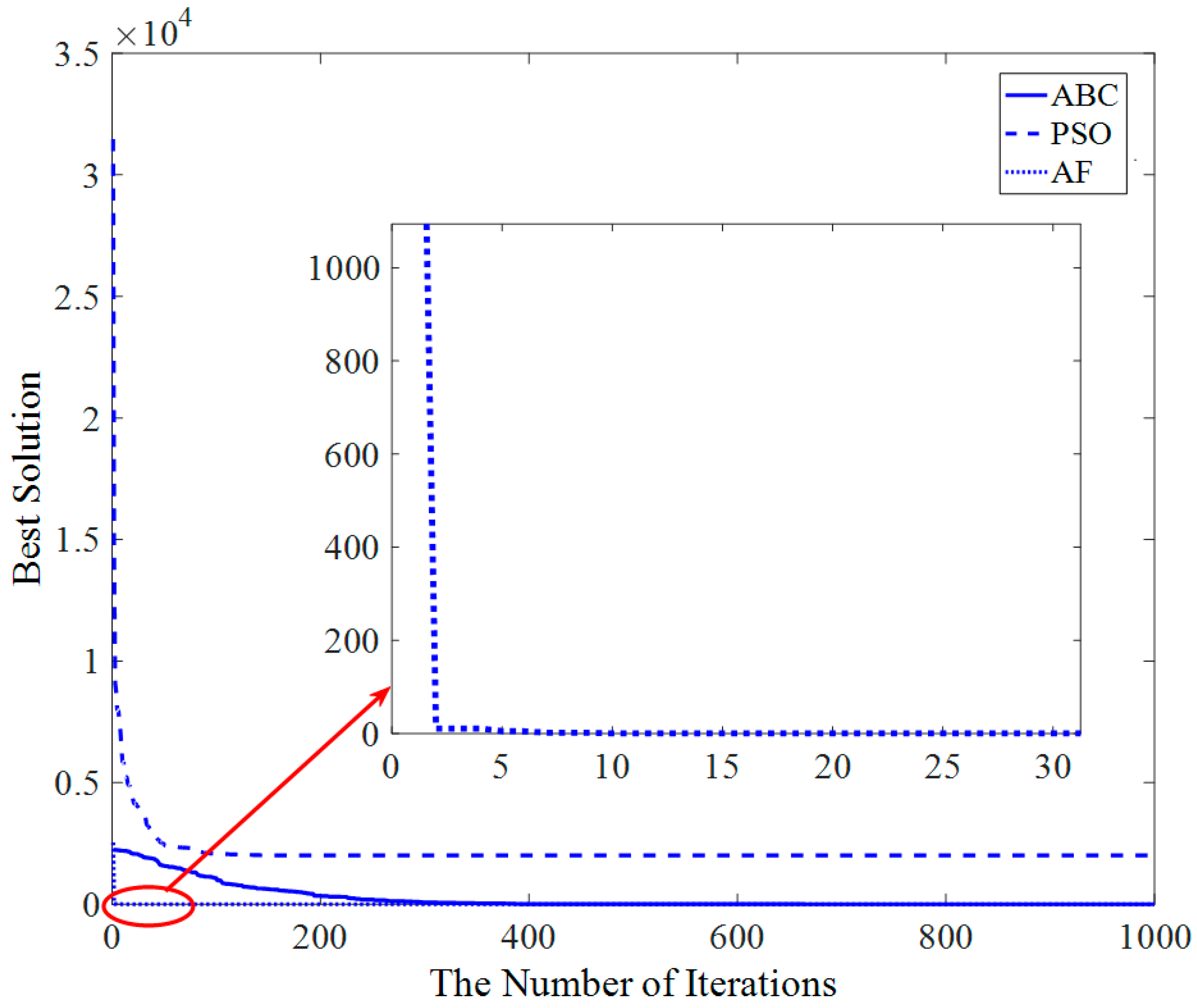
Figure 20.
The convergence curve of the three algorithms for Ackley function in 100-dimensional space.
Figure 20.
The convergence curve of the three algorithms for Ackley function in 100-dimensional space.

Table 1.
Pseudo code of artificial flora algorithm.
| Input: times: Maximum run time M: Maximum branching number N: Number of original plants p: survival probability of offspring plants t = 0; Initialize the population and define the related parameters Evaluate the N individuals’ fitness value, and find the best solution While (t < times) For i = 1:N*M New original plants evolve propagation distance (According to Equation (1), Equation (2) and Equation (3)) Original plants spread their offspring (According to Equation (5)) If rand(0,1) >p Offspring plant is alive Else Offspring is died End if End for Evaluate new solutions, and select N plants as new original plants randomly. If the new solutionis better than their previous one, new plant will replace the old one. Find the current best solution t = t + 1; End while Output: Optimal solution |
Table 2.
The time complexity of artificial flora algorithm.
| Operation | Time | Time Complexity |
|---|---|---|
| Initialize | N × t1 | O(N) |
| Calculate propagation distance | 2N × t2 | O(N) |
| Update the position | N × t3 | O(N) |
| Calculate fitness | N × M × t4 | O(N·M) |
| Calculate survival probability | N × M × t5 | O(N·M) |
| Decide alive plant using roulette | N × M × t6 | O(N·M) |
Table 3.
Benchmark functions.
| Functions | Expression formula | Bounds | Optimum Value |
|---|---|---|---|
| Sphere | [−100,100] | 0 | |
| Rosenbrock | [−30,30] | 0 | |
| Rastrigin | [−5.12,5.12] | 0 | |
| Schwefel | [−500,500] | −418.9829 × D | |
| Griewank | [−600,600] | 0 | |
| Ackley | [−32,32] | 0 |
Table 4.
The default parameters in particle swarm optimization (PSO), artificial bee colony (ABC), and artificial flora (AF) algorithms.
Table 4.
The default parameters in particle swarm optimization (PSO), artificial bee colony (ABC), and artificial flora (AF) algorithms.
| Algorithm | Parameter Values |
|---|---|
| PSO | N = 100,c1 = c2 = 1.4962,w = 0.7298 |
| ABC | N = 200,limit = 1000 |
| AF | N = 1,M = 100,c1 = 0.75,c2= 1.25 |
Table 5.
Comparison of statistical results obtained by AF, PSO, and ABC in 20-dimensional space.
| Functions | Algorithm | Best | Mean | Worst | SD | Runtime |
|---|---|---|---|---|---|---|
| Sphere | PSO | 0.022229639 | 10.36862151 | 110.8350423 | 21.05011998 | 0.407360 |
| ABC | 2.22518 × 10⁻¹⁶ | 3.03501 × 10⁻¹⁶ | 4.3713 × 10⁻¹⁶ | 5.35969 × 10⁻¹⁷ | 2.988014 | |
| AF | 0 | 0 | 0 | 2.536061 | ||
| Rosenbrock | PSO | 86.00167369 | 19,283.23676 | 222,601.751 | 43,960.73321 | 0.578351 |
| ABC | 0.004636871 | 0.071185731 | 0.245132443 | 0.065746751 | 3.825228 | |
| AF | 17.93243086 | 18.44894891 | 18.77237391 | 0.238206854 | 4.876399 | |
| Rastrigin | PSO | 60.69461471 | 124.3756019 | 261.6735015 | 43.5954195 | 0.588299 |
| ABC | 0 | 1.7053 × 10⁻¹⁴ | 5.68434 × 10⁻¹⁴ | 1.90442 × 10⁻¹⁴ | 3.388325 | |
| AF | 0 | 0 | 0 | 0 | 2.730699 | |
| Schwefel | PSO | −1.082 × 10105 | −2.0346 × 10149 | −1.0156 × 10151 | 1.4362 × 10150 | 1.480785 |
| ABC | −8379.657745 | −8379.656033 | −8379.618707 | 0.007303823 | 3.462507 | |
| AF | −7510.128926 | −11,279.67966 | −177,281.186 | 25,371.33579 | 3.144982 | |
| Griewank | PSO | 0.127645871 | 0.639982775 | 1.252113282 | 0.31200235 | 1.097885 |
| ABC | 0 | 7.37654 × 10⁻¹⁴ | 2.61158 × 10⁻¹² | 3.70604 × 10⁻¹³ | 6.051243 | |
| AF | 0 | 0 | 0 | 0 | 2.927380 | |
| Ackley | PSO | 19.99906463 | 20.04706409 | 20.46501638 | 0.103726728 | 0.949812 |
| ABC | 2.0338 × 10⁻¹⁰ | 4.5334 × 10⁻¹⁰ | 1.02975 × 10⁻⁹ | 1.6605 × 10⁻¹⁰ | 3.652016 | |
| AF | 8.88 × 10⁻¹⁶ | 8.88 × 10⁻¹⁶ | 8.88 × 10⁻¹⁶ | 0 | 3.023296 |
Table 6.
Comparison of statistical results obtained by AF, PSO, and ABC in 50-dimensional space.
| Functions | Algorithm | Best | Mean | Worst | SD | Runtime |
|---|---|---|---|---|---|---|
| Sphere | PSO | 13,513.53237 | 29,913.32912 | 55,187.50413 | 9279.053897 | 0.515428 |
| ABC | 6.73535 × 10⁻⁸ | 3.56859 × 10⁻⁷ | 1.17148 × 10⁻⁶ | 2.37263 × 10⁻⁷ | 3.548339 | |
| AF | 0 | 4.22551 × 10⁻³² | 2.11276 × 10⁻³⁰ | 2.95786 × 10⁻³¹ | 3.476036 | |
| Rosenbrock | PSO | 9,137,632.795 | 53,765,803.92 | 313,258,238.9 | 49,387,420.59 | 0.707141 |
| ABC | 0.409359085 | 13.87909385 | 49.83380808 | 9.973291581 | 4.094523 | |
| AF | 47.95457 | 48.50293 | 48.87977 | 0.246019 | 6.674920 | |
| Rastrigin | PSO | 500.5355119 | 671.5528998 | 892.8727757 | 98.8516628 | 1.036802 |
| ABC | 0.995796171 | 3.850881679 | 7.36921061 | 1.539235109 | 3.661335 | |
| AF | 0 | 0 | 0 | 0 | 3.753900 | |
| Schwefel | PSO | −1.6819 × 10127 | −5.9384 × 10125 | −2.5216 × 10⁵ | 2.7148 × 10126 | 2.672258 |
| ABC | −20,111.1655 | −19,720.51324 | −19,318.44458 | 183.7240198 | 3.433517 | |
| AF | −20,680.01223 | −23,796.53666 | −93,734.38905 | 16,356.3483 | 4.053411 | |
| Griewank | PSO | 118.8833865 | 283.810608 | 524.5110849 | 101.3692096 | 1.609482 |
| ABC | 1.63 × 10⁻⁶ | 1.29 × 10⁻³ | 3.30 × 10⁻² | 0.005265446 | 6.573567 | |
| AF | 0 | 0 | 0 | 0 | 3.564724 | |
| Ackley | PSO | 20.169350 | 20.452818 | 21.151007 | 0.2030427 | 1.499010 |
| ABC | 0.003030661 | 0.009076649 | 0.033812712 | 0.005609339 | 4.315255 | |
| AF | 8.88 × 10⁻¹⁶ | 8.88 × 10⁻¹⁶ | 8.88 × 10⁻¹⁶ | 0 | 5.463588 |
Table 7.
Comparison of statistical results obtained by AF, PSO, and ABC in 100-dimensional space.
| Functions | Algorithm | Best | Mean | Worst | SD | Runtime |
|---|---|---|---|---|---|---|
| Sphere | PSO | 115,645.5342 | 195,135.2461 | 278,094.825 | 38,558.16575 | 0.711345 |
| ABC | 0.000594137 | 0.001826666 | 0.004501827 | 0.000839266 | 3.461872 | |
| AF | 0 | 3.13781 × 10⁻¹⁶ | 1.34675 × 10⁻¹⁴ | 1.88902 × 10⁻¹⁵ | 5.147278 | |
| Rosenbrock | PSO | 335,003,051.6 | 886,456,293.7 | 2,124,907,403 | 386,634,404.3 | 1.053024 |
| ABC | 87.31216327 | 482.9875993 | 3159.533172 | 660.8862246 | 4.249927 | |
| AF | 98.16326 | 98.75210 | 98.91893 | 0.143608 | 9.205695 | |
| Rastrigin | PSO | 1400.13738 | 1788.428575 | 2237.676158 | 190.5442307 | 1.711449 |
| ABC | 38.31898075 | 57.90108742 | 71.66147576 | 7.625052886 | 4.177761 | |
| AF | 0 | 3.55271 × 10⁻¹⁷ | 1.77636 × 10⁻¹⁵ | 2.4869 × 10⁻¹⁶ | 5.526152 | |
| Schwefel | PSO | −1.8278 × 10130 | −3.6943 × 10128 | −9.38464 × 1085 | 2.5844 × 10129 | 4.541757 |
| ABC | −36,633.02634 | −35,865.45846 | −35,018.41908 | 428.4258428 | 3.776740 | |
| AF | −42,305.38762 | −43,259.38057 | −212,423.8294 | 42,713.19955 | 5.638101 | |
| Griewank | PSO | 921.4736939 | 1750.684535 | 2954.013327 | 393.6416257 | 2.117832 |
| ABC | 0.006642796 | 0.104038042 | 0.349646578 | 0.098645373 | 6.995976 | |
| AF | 0 | 1.71 × 10⁻¹¹ | 4.96314 × 10⁻¹⁰ | 7.66992 × 10⁻¹¹ | 5.440354 | |
| Ackley | PSO | 20.58328517 | 20.83783825 | 21.17117933 | 0.152682198 | 2.011021 |
| ABC | 2.062017063 | 2.669238251 | 3.277291002 | 0.28375453 | 4.611272 | |
| AF | 8.88 × 10⁻¹⁶ | 8.88 × 10⁻¹⁶ | 8.88 × 10⁻¹⁶ | 0 | 6.812734 |
© 2018 by the authors. Licensee MDPI, Basel, Switzerland. This article is an open access article distributed under the terms and conditions of the Creative Commons Attribution (CC BY) license (http://creativecommons.org/licenses/by/4.0/).
Share and Cite
MDPI and ACS Style
Cheng, L.; Wu, X.-h.; Wang, Y. Artificial Flora (AF) Optimization Algorithm. Appl. Sci. 2018, 8, 329. https://doi.org/10.3390/app8030329
AMA Style
Cheng L, Wu X-h, Wang Y. Artificial Flora (AF) Optimization Algorithm. Applied Sciences. 2018; 8(3):329. https://doi.org/10.3390/app8030329
Chicago/Turabian StyleCheng, Long, Xue-han Wu, and Yan Wang. 2018. "Artificial Flora (AF) Optimization Algorithm" Applied Sciences 8, no. 3: 329. https://doi.org/10.3390/app8030329
Note that from the first issue of 2016, this journal uses article numbers instead of page numbers. See further details here.