A Lattice Boltzmann Method and Asynchronous Model Coupling for Viscoelastic Fluids


1
School of Science, Xi’an Polytechnic University, Xi’an 710048, China
2
School of Science, Northwestern Polytechnical University, Xi’an 710129, China
*
Authors to whom correspondence should be addressed.
Appl. Sci. 2018, 8(3), 352; https://doi.org/10.3390/app8030352
Submission received: 21 January 2018
/
Revised: 23 February 2018
/
Accepted: 26 February 2018
/
Published: 28 February 2018
(This article belongs to the Special Issue Development and Applications of Kinetic Solvers for Complex Flows)
Abstract
:The numerical algorithms of viscoelastic flows can appear a tremendous challenge as the Weissenberg number (Wi) enlarged sufficiently. In this study, we present a generalized technique of time-stably advancing based on the coupled lattice Boltzmann method, in order to improve the numerical stability of simulations at a high Wi number. The mathematical models of viscoelastic fluids include both the equation of the solvent and the Oldroyd-B constitutive equation of the polymer. In the two-dimensional (2D) channel flow, the coupled method shows good agreements between the corresponding exact results and the numerical results obtained by our method. In addition, as the Wi number increased, for the viscoelastic flows through contractions, we show that the prediction of our presented method can reproduce the same numerical results that were reported by previous studies. The main advantage of current method is that it can be applied to simulate the complex phenomena of the viscoelastic fluids.
1. Introduction
Over the last few decades, there has been substantial development in the numerical simulation of viscoelastic fluids, which are commonly encountered in many important industries, such as oil and chemical engineering. However, the numerical solution of the viscoelastic constitutive models is a tremendous challenge, due to breakdown in convergence of algorithms when the Weissenberg number (Wi, is a non-dimensional number characterizing the effect of elasticity on the flow) is increased [1,2]. At large levels of elasticity, the stress field often contains stress singularities at sharp corners or stagnation points [3]. Many researchers have already had some attempts to develop robust and stable numerical algorithm to solve viscoelastic fluid flows at moderately high values of Wi number, such as discontinuous Galerkin method [4], finite-volume methods [5,6,7], and the lattice Boltzmann method. Among the various numerical methods of the viscoelastic fluids in literatures, the lattice Boltzmann method (LBM) [8,9,10] has attracted much attention due to its kinetic nature for modeling the complex fluids.
Since 1990s, Qian [11] and Giraud [12] have been developed the lattice Boltzmann method to account for non-Newtonian behaviors, but they did not focus on the model with strong elastic effects. Later, several approaches have been proposed to incorporate constitutive equations in lattice Boltzmann simulations for viscoelastic fluids [13,14,15,16,17]. Recently, Papenkort et al. [18] investigated viscoelastic shear-thinning fluid using lattice Boltzmann method; Wang et al. [19] employed a multiple-relaxation-time lattice Boltzmann flux solver for non-Newtonian power-law fluid flows. Xie et al. [20] extended a lattice Boltzmann method scheme to multiphase viscoplastic fluids by applying the Herschel-Bulkley constitutive relationship. It is worth mentioning that a coupled lattice Boltzmann method have been devised to solve the equations of an Oldroyd-B viscoelastic fluid in the reference [21], which did not need to adding extra distribution functions for the stress tensor. The coupled systems of the viscoelastic fluid include the macro scale constitutive equation and the mesoscopic lattice Boltzmann equation. There is a more disparity in timescales between the macro solver and meso solver. To distinguish this different time scale and enhance the computational efficiency, the asynchronously coupled method [22,23] was applied for the coupling time in reference [21]. That means, the data between macro constitutive equation and the lattice Boltzmann equation exchange at every time step. The constitutive solver may run at a slower pace than the meso-scale dynamics.
The asynchronous coupling method allows for the coupled solvers to exchange the data at every loop, although the meso and macro time steps are unequal. This special treatment is actually a numerical approximation to the true solution. For viscoelastic fluids at low Wi number, asynchronously coupled method may get steady result in simulations if the macro time step can guarantee the adequate resolutions of each solvers because of the small scale-separation. However, for viscoelastic fluids at high Wi number, the computational stability of asynchronously coupling is greatly affected by the polymer stress as the elasticity interaction becomes relatively large. Therefore, the asynchronously coupling method has the limitations, such as poor numerical stability, which were limited to solve the low Wi number problem.
The aim of the current paper is to develop a generalized technique for time advancing of the viscoelastic coupled lattice Boltzmann method, seeking to be immune to high Wi number problem. The basic idea of our new method is as follows. (i) Run the lattice Boltzmann solver using its own time step , while allowing for a flexible number of lattice Boltzmann solver steps N before the exchange of coupling variables; (ii) Run the constitutive solver using its own time step . (iii) Exchange data between the lattice Boltzmann and constitutive solvers. Note that, the number of flexible steps, N, provides an additional control of the coupling. This skill enables the applicability of the coupled lattice Boltzmann method at high Wi number, while minimizing the number of lattice Boltzmann and constitutive time steps needed. We refer to this method as a generalized asynchronously coupling method. This article is organized as follows: Section 2 describes the mathematical models that are used in the simulation of viscoelastic fluids. In Section 3, we give the coupled lattice Boltzmann scheme of an Oldroyd-B viscoelastic fluid and the details of the generalized asynchronously coupling method. In Section 4, we show the results of simulations for viscoelastic fluids at high Wi number using the generalized method. Finally, we give the conclusions of this paper and some future prospects.
2. The Descriptions of Mathematical Models
In the simulations, we use the Oldroyd-B constitutive model to describe the elasticity effect of viscoelastic fluids, in which the polymer molecules are modeled by the two beads connected by a spring [24]. We treat the solvent of the viscoelastic model as an incompressible flow at low Reynolds number. The equations of the momentum and mass conservation are given by
where , , , represent, respectively, the velocity, the density, pressure, and solvent viscosity. is the extra-stress tensor accounting for the viscoelastic effects of the stretching and the relaxation of the polymer macro-molecules diluted in the solvent. The constitutive equation of the Oldroyd-B model reads
where the , the superscript “T” and denote, respectively, the material derivative, transpose operation and the rate of strain tensor; , are the relaxation time of polymer solutions and the dynamic viscosity of the polymer, respectively. In the simulations, we present all the data in non-dimensional forms, normalized in terms of the characteristic length L and the characteristic velocity U (characteristic time is L/U). Weissenberg (Wi) number is defined by to characterize the viscoelastic effect for shear flows. The Reynolds number, Re, is defined as , respectively. The parameter is the ratio of the solvent viscosity to total viscosity, is the total viscosity. Finally, we get , .
3. The Coupled LBM of Viscoelastic Fluids
We will briefly describe the numerical implementations simulating the viscoelastic fluids in this section. The two-dimensional (2D) incompressible lattice Boltzmann method is utilized to solve the equations of the solvent. In order to avoid adding a new set of distribution functions, the constitutive equation is split into the relaxation-stretching and advection operators, where the advection operator of the stress tensor is directly solved by implementing the particle distribution functions of solvent. Specifically, to seek the coupled LBM that can be immune to high Wi number problem, we develop a generalized asynchronously coupled method of advancing the time step. All of these details will be described as follow.
3.1. Incompressible LBGK Model with the Extra Force
In this study, we use the 2D incompressible Lattice Boltzmann Bhatnagar-Gross-Krook (LBGK) model [25] based on the two-dimensional nine velocity (D2Q9) model to recover the Navier-Stokes equations. The particle velocity may be written as
here, , are, respectively, the lattice grid spacing and the time step, represents the particle velocity.
The lattice Boltzmann equation (LBE) reads
where denotes the distribution function at the node of at the time , and the BGK collision model, , is given by
where represents the dimensionless relaxation time, is relaxation time. The equilibrium distribution function (EDF), , is given by
where
and are the velocity and the fluid pressure, respectively. The weight coefficients are
here represents the acoustic speed, is a constant of density. The pressure and velocity of flow are deduced from the ensemble average of distribution functions
In the simulation of viscoelastic fluids, the treatment of the elastic force may be crucial for the coupled lattice Boltzmann method. Here, we incorporate the extra forces into lattice Boltzmann equation, and treat the elastic force of polymers as an extra forced of the lattice Boltzmann BGK [26]. The incompressible LBGK Equation (5) with the additional elastic forced term is updated by
where the equilibrium distribution is updated by
with
the right-hand-side term is given by
where
The flow velocity is finally updated by averaging the value of the after and fore collision
The incompressible Navier-Stokes Equations (1) and (2) could be derived from lattice Boltzmann Equation (12) using the Chapman-Enskog expansion, with the kinematic viscosity . Detailed mathematical deduce is given in the Appendix A.
3.2. Solving the Oldroyd-B Constitutive Model
In this section, we describe briefly the way to solve the Oldroyd-B Equation (3) using the particle distribution functions of flow fields. To check the information conveniently, we rewrite the constitutive equation as
here, the advection operator and relaxation-stretching operator acted on the stress tensor are given, respectively, by
Here, the physical variables of the Equations (19) and (20) are distributed on the same grid points as the velocity field. To ensure the numerical precision of simulation, the advection operator is calculated by
The relaxation-stretching operators are stretched through the velocity gradient tensor. The derivatives of velocity are computed by
In the simulation, the time stepping follows as
Here, the time step may normally be different from , and the velocity field is fixed during the time when the constitutive equation advance from n to n + 1 time step. Finally, combing with the Equations (21) and (23), we obtained the temporal advancing of the stress tensor, as follows
The detail derivation of the numerical scheme is has been shown in the in reference [21].
3.3. The Temporal Marching of Coupled Solvers
The computing steps of the velocity and viscoelastic stress fields are arranged as follows: (I) Equation (24) are run firstly to simulate the constitutive equations, of whose results are utilized to calculate the elastic forces; (II) The velocity fields are simulated using Equation (14), and the obtained results are utilized to calculate the related velocity gradient; (III) The velocity and elastic stress fields are updated iteratively at each step.
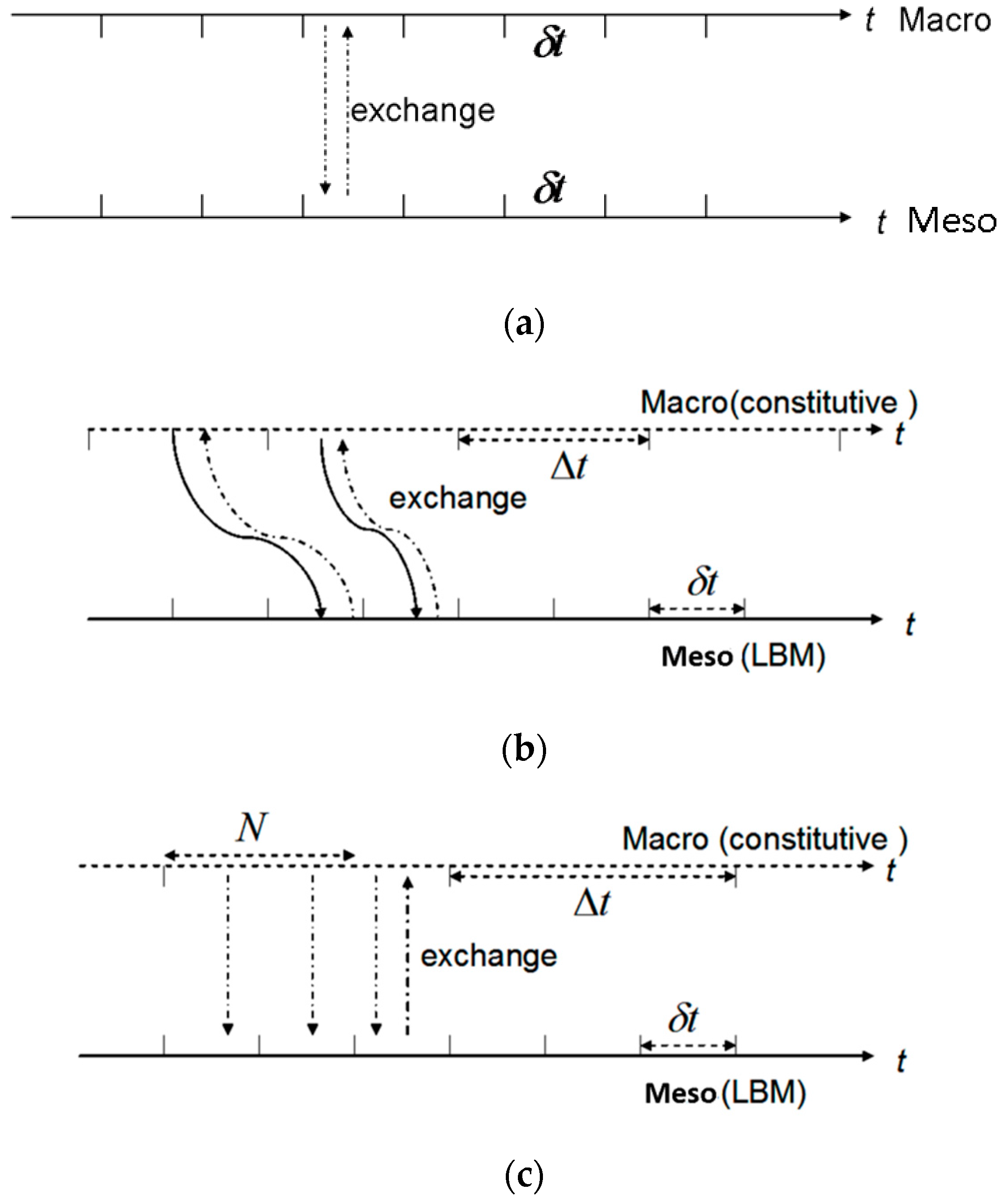
In this part, we mainly discuss the methods of time marching in coupled solvers. For viscoelastic fluid flows at low Re number, the coupled systems have a very huge difference of the time scales between the constitutive modes and lattice Boltzmann evolution. So, we must carefully handle with the time scale when simulating the real geometry device. One approach to time advancement in a coupled framework is to operate the solvers at the smallest scale that required by the lattice Boltzmann equation. However, the computational cost will normally be much larger than it needed. Such a type of method is displayed in Figure 1a and we named it as the fully coupled (FC) method. To improve the efficiency of simulations, the asynchronously coupled method was applied in previous work [21]. There are two time steps being used in this coupled framework. The lattice Boltzmann equation runs by the suitable time step corresponding to its physical model, but the macro constitutive equations are solver with fewer numbers of time steps (with larger time-step sizes) than the mesoscale dynamics. The named asynchronously coupled methods mean that the data exchange mode between the lattice Boltzmann equation and macro constitutive equation at every time step. On a separate note, the numerical error that was caused by the scale-separated method may be acceptable if the time step of the macro constitutive is chosen properly. This method is shown schematically in Figure 1b and we refer to it as the asynchronously coupled (AC) method. The coupled algorithm using a homogeneous time step is given, as following Algorithm 1.
| Algorithm 1. The coupled algorithm using a homogeneous time step. |
| Require: , , , , (is a dimension less terminal time) |
| Do |
| ; |
| ; |
| ; |
| ; |
| ; |
| ; |
| While |
For viscoelastic fluids at low Wi number, the asynchronous time marching of the coupled solvers could get steady result in simulations if the macro time step is chosen properly. However, as Wi number increases, the asynchronously coupled method possesses fairly poor numerical stability. To widen the application of the coupled lattice Boltzmann model, we propose a generalized asynchronously coupled method for time-stably advancing of the viscoelastic lattice Boltzmann method. In this method, the asynchronously coupled way adding an iterative procedure is performed, which may allow for the lattice Boltzmann solver to run with a flexible number of steps (N) before the exchange of coupling variables. The number of added steps, N, gives a further role to relax the coupling instances system. We refer to this method as the generalized asynchronously coupling (GAC) method (see Figure 1c), which can extend the applicability over a wide range of Wi number. The similar ideas have been used in literature [27] where the disparate time scales were applied to study dynamical systems. In brief, the procedure of the generalized asynchronously coupling method is given as following Algorithm 2.
| Algorithm 2. Generalized asynchronously coupling method. |
| Require: , , , , (is a dimension less terminal time) |
| Do |
| For (k = 1; k++; k ≤ N) |
| { |
| ; |
| } |
| ; |
| ; |
| ; |
| ; |
| While |
It’s should be noted at that the GAC scheme we presented in this paper is equivalent to the AC scheme (used in [21]) when N = 1. The flexibility that is provided through the assignment of N enables the best of these methods to be combined in an adaptable manner. In this paper the assignment of N is made as straightforwardly as possible: to minimise the number of macro time steps performed. As such, it is set as large as the restriction on macro time step will allow. This inherent adaptability gives the GAC scheme the range of applicability of the AC method, while maintaining the macro-time-step efficiency as much as possible.
4. Numerical Results and Discussions
The generalized asynchronously coupled method is first validated by a planar channel flow. Subsequently, to prove reliability of the coupled solvers, the 4:1 contraction problem is also implemented in the simulation. We will give the detail numerical results as follow.
4.1. 2D Channel Flows
In order to verify the numerical accuracy of coupled solvers, we choose a 2D channel shaped by two parallel panels over distance of about L with H = 10L long (see Figure 2). The characteristic length L and the characteristic velocity U are the height and maximum velocity of at the inlet, respectively.
The velocity boundary conditions paralleled to the x-axis wall are, respectively,
The boundary conditions of stress paralleled to the x-axis wall could be obtained by velocity values. The Neumann boundary conditions at the exit are, respectively, used as follows
The stress tensor values are initially imposed to zero everywhere, and the fully-developed conditions are used at the entry, which is taken by
then the maximum velocity at the inlet is U = 0.1.
The Oldroyd-B constitutive equation has an exact solution when the velocity field has reached the steady state, which is written by
So, we also can study the numerical precision of the presented method by comparing with the exact solution. The relative errors of numerical solutions for stress based on the L2-norm are given by
where M is the total number of nodes, , denote the steady-state numerical solutions and , are the exact solutions.
Generally speaking, at low Wi number, asynchronously coupled method can get a stability result in simulations only if the and can guarantee the adequate resolutions of each solvers because of the small scale-separation. The value of N is related with the ratio of time-step sizes , but is usually not linear with respect to it. In practical applications, N is found by the trial and error approach. For instance, we initially set N0 = 2h, , present round to ceiling. We can take N = N0, if the iterative error of was decreased when N = N0, other else we use N0 = 2h+1 to test once again, and so on. We first run simulations using and with the fined mesh of 400 × 40, and N = 5 for generalized asynchronously coupled method, at lower Wi = 1, and get the results in the Figure 3, comparing AC scheme with GAC scheme. We find that despite both AC scheme and GAC scheme can get a stability result in simulations, the convergence speed of GAC scheme is fast than the AC scheme.
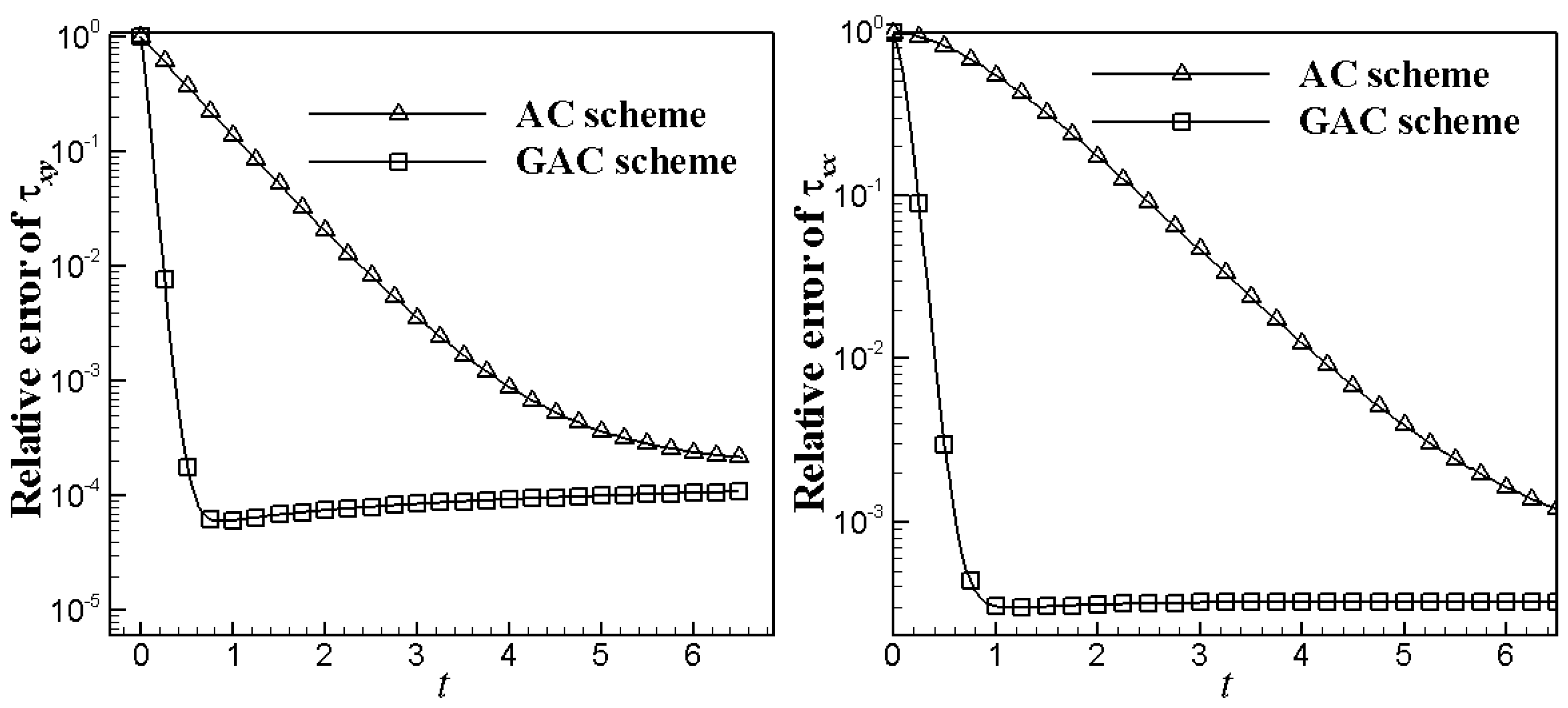
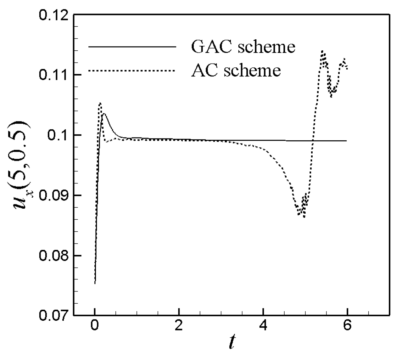
To show the validity of the generalized asynchronously coupled method, we then take the dimensionless units as 0.1, as 1, Wi = 15.0, parameter as 0.5, and = 1, Re number as 1.0, then , , and compare the numerical results of our method with the analytical solution and asynchronously coupled scheme. We also set and for coupled using the fined mesh of 400 × 40, and N = 5 for generalized asynchronously coupled method. Figure 4 shows that the relative error of and simulated by our present scheme is extremely small at Wi = 15, whereas the relative error of obtained by asynchronously scheme is clearly exceeded more than 100%. In other words, the asynchronously coupled method is considerably subject to numerical error at Wi = 15. Nevertheless, when comparing with the standard asynchronously coupled methods, the generalized method persists to give stable solutions up to Wi = 15. Overall, seeing from the analysis of relative error, we found that the present method could be immune to problem of Wi = 15. Moreover, we plot the velocity components u, as obtained by numerical method at centre point (5, 0.5) on time t in Figure 5, comparing with the results of the asynchronously coupled method at and Re = 1.0. From Figure 5, we found that, before eventually reaching a steady state, the velocity profiles overshoot the terminal velocity due to the action of the elasticity. However, the result of the asynchronously coupled method is divergent as the time increasing because of its poor stability.
4.2. Contraction Flows
Viscoelastic fluids through contractions are important in the rapidly developed research field of micro fluidics, such as the polymer processing. As we know, the contraction flow has singularity at the reentrant corner, which makes calculations at high Weissenberg numbers challenging. The planar 4:1 contraction was seen as a benchmark [28] model in 1987 because of the geometrical simplicity and the known numerical difficulty. In this section, to further test the validity of the method presented in this paper, we simulate the Oldroyd-B fluids through a 4:1contraction geometry at Wi = 5.
Figure 6 shows the flow domain of which the ratio between the downstream and upstream height is 1 to 4. The characteristic length L and the characteristic velocity U are the half height and average velocity at the outlet, respectively. A parabolic Poiseuille flow is set at inflow by
while the fully-developed conditions are given at the outlet, so the average velocity U at the out let is 1. No-slip boundary conditions are given along the stationary walls. Symmetry boundary conditions are imposed along the center-line. We take the dimensionless units U as 1, as 1, parameter as , and Re number as 1.0.
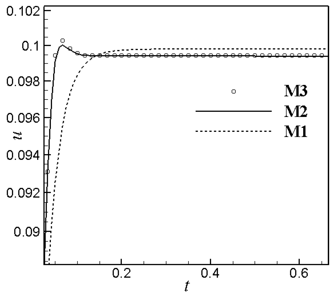
To verify the mesh convergence, we carried out the calculations of a steady flow with using three Cartesian meshes, M1, M2 and M3. The total number of cells and the grid size of each mesh are reported in Table 1. Figure 7 displays the temporal evolution of the local velocity at the intersection of the symmetry line and the contraction plane of the channel, for the different mesh. From Figure 7, we can see that the velocity tends to be meshing independent as the number of the nodes increased. To juggle the computational precision and efficiency, the numerical results are got in the next parts by utilizing the dense mesh of M3. For the generalized asynchronously coupled method, we set , and N = 4. Figure 8 displays the numerical results of velocity components along the horizontal center lines of the contraction with Wi = 1.0, comparing between the results of GAC and AC method, respectively. We can see that the difference of those two schemes is not obvious at low Wi number flows. That study of low Wi number flows is a benchmark example when considering it as a preview to the high Wi number flows in the following part.
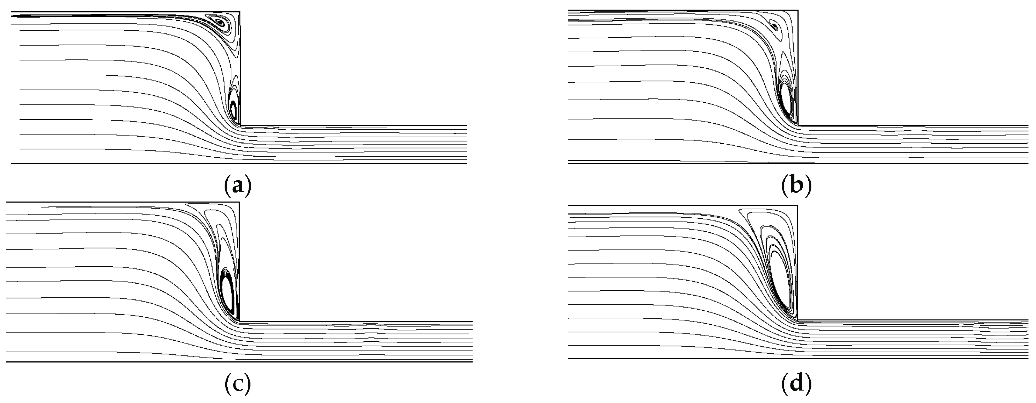
To obtain some complex viscoelastic behaviors, we consider the dynamics of viscoelastic fluids at Wi = 5.0 using the GAC in this part. Figure 9 displays a set of instantaneous streamlines of flows with Wi = 5.0 on the finest mesh M3. Concerning the dynamics of viscoelastic fluids, we can find a series of different flow regimes, while increasing the Wi number to 5.0. From Figure 9, we observe that the elastic lip vortex grows in size as time goes by, eventually running up to the corner vortex region, and mixing with each other in a fairly complex dynamic process. The dynamical transitions are signed by a complex interaction between pulsating lip and corner vortices, which tend to approach and separate. In the literatures, through a full 4:1 planar contraction, Comminal et al. [5] and Afonso et al. [29], by carrying out numerical simulations of the Oldroyd-B model, also predicted the similar coalescence of lip and salient corner vortices into one big vortex with increasing elasticity. When comparing quantitatively with the previous works, we find that the prediction of our presented method reproduces the numerical results reported in the previous studies. However, under the same condition, the procedure using the AC scheme does not obtain the converged solution as the Wi number increases to 5.0. Overall, thorough the stringent test case, we have found that the generalized coupled lattice Boltzmann method could be fit to simulate the Oldroyd-B fluids when the Wi number is increased.
5. Conclusions
In conclusions, we have employed a coupled lattice Boltzmann method, with a generalized asynchronously coupling scheme, to simulate the Oldroyd-B fluids when the Weissenberg number is increased. This coupled method includes two types of equations, one is Lattice Boltzmann equation of the solvent and the other is constitutive equation of the stress tensor. The two equations are solved using two different time steps—one is of macroscopic scale and the other is of mesoscopic scale. For viscoelastic fluids at a higher Wi number, the computational stability of asynchronously coupling is greatly affected by the polymer stress as the elasticity interaction becomes relatively large. Therefore, we have presented a generalized technique for time-stably advancing of the coupled lattice Boltzmann method, which can improve the numerical stability of the simulation at a higher Wi number. The main idea of the new method is that one can add an adaptable number of micro solver time steps before the transmission of data between the coupling variables.
We have shown that the numerical results, as calculated by the new method, are in good agreement with analytical results of the two-dimensional channel flow. In addition, for viscoelastic fluids through contractions at Wi = 5, we have found that the prediction of our presented method can reproduce the same numerical results that were obtained by previous literatures. The main advantage of our presented method is that it could be use to simulate the Oldroyd-B fluids when the Wi number is increased. Furthermore, our new method could also be easily implemented, which keeps the traditional advantageous of LBM. Hence, the coupled lattice Boltzmann method that was described in this paper could be seen as an alternative numerical technique for simulating the viscoelastic fluid.
Acknowledgments
This work was supported by the National Natural Science Foundation of China (Grant Nos. 11601411,11601410), the Natural Science Basic Research Plan in Shaanxi Province of China (Program No. 2017JQ1029), the Scientific Research Program Funded by Shaanxi Provincial Education Department (Program No. 15JK1313), and the Scientific Research Foundation of Xi’an Polytechnic University (BS1435).
Author Contributions
Jin Su developed the numerical method, analyzed the data and drafted the manuscript. Jie Ouyangconceived of the study and finalized the manuscript. Junxiang Luperformed the scratch numerical experiments, and edited the manuscript. All the authors read and approved the final version of the manuscript.
Conflicts of Interest
The authors declare no conflict of interest.
Appendix A. Recovering Incompressible Naveier-Stokes Equation with Elastic Force
To derive the macroscopic Equations (1) and (2), the Chapman-Enskog expansion in time and space is implemented
Here, is a small expansion parameter.
Using Taylor expansion to evolution Equation (12), we have
where , Denote . Substituting Equations (A1) and (A2) into Equation (A3) and treating the terms in order of , and separately gives
According to Equations (A5) and (A6) and collecting the terms related to on the both sides, we can rewrite Equation (A6) as
According to Equation (A4), we obtain
Then, we get
According to Equations (A8) and (A9), we get
To recover the Euler equations from Equation (1), we choose .
Taking moments of Equation (A5), we can obtain the following macroscopic equations on the t1 time scale
where
The first-order momentum flux can be simplified using (A12) and (A13)
After some standard algebra, we obtain that
where the terms of order or higher have been neglected.
Combining the results on the t0 and t1 time scales, we get
where .
To eliminate the unexpected effects, we take , and obtain the final macroscopic equations:
where , .
References
- Keunings, R. On the high Weissenberg number problem. J. Non-Newton. Fluid Mech. 1986, 20, 209–226. [Google Scholar] [CrossRef]
- Walters, K.; Webster, M.F. The distinctive CFD challenges of computational rheology. Int. J. Numer. Methods Fluids 2003, 43, 577–596. [Google Scholar] [CrossRef]
- Renardy, M. Current issues in non-Newtonian flows: A mathematical perspective. J. Non-Newton. Fluid Mech. 2000, 90, 243–259. [Google Scholar] [CrossRef]
- Mirzakhalili, E.; Nejat, A. High-order solution of viscoelastic fluids using the discontinuous Galerk in method. J. Fluids Eng. 2015, 137, 031205. [Google Scholar] [CrossRef]
- Comminal, R.; Hattel, J.H.; Alves, M.A.; Spangenberg, J. Vortex behavior of the Oldroyd-B fluid in the 4-1 planar contraction simulated with the stream function–log-conformation formulation. J. Non-Newton. Fluid Mech. 2016, 237, 1–15. [Google Scholar] [CrossRef]
- Niethammer, M.; Marschall, H.; Kunkelmann, C.; Bothe, D. A numerical stabilization framework for viscoelastic fluid flow using the finite volume method on general unstructured meshes. Int. J. Number. Methods Fluids 2017, 86, 131–166. [Google Scholar] [CrossRef]
- Pimenta, F.; Alves, M.A. Stabilization of an open-source finite-volume solver for viscoelastic fluid flows. J. Non-Newton. Fluid Mech. 2017, 239, 85–104. [Google Scholar] [CrossRef]
- Chen, S.; Doolen, G.D. Lattice Boltzmann method for fluid flows. Ann. Rev. Fluid Mech. 1998, 30, 329–364. [Google Scholar] [CrossRef]
- Qian, Y.H.; d’Humières, D.; Lallemand, P. Lattice BGK Models for Navier-Stokes Equation. Europhys. Lett. 1992, 17, 479–484. [Google Scholar] [CrossRef]
- Succi, S. The Lattice Boltzmann Equation for Fluid Dynamics and Beyond; Oxford University Press: Oxford, MS, USA, 2001. [Google Scholar]
- Qian, Y.H.; Deng, Y.F. A lattice BGK model for viscoelastic media. Phys. Rev. Lett. 1997, 79, 2742–2745. [Google Scholar] [CrossRef]
- Giraud, L.; d’Humières, D.; Lallemand, P. A lattice Boltzmann model for Jeffreys viscoelastic fluid. Euro Phys. Lett. 1998, 42, 625–630. [Google Scholar] [CrossRef]
- Ammar, A. Lattice Boltzmann method for polymer kinetic theory. J. Non-Newton. Fluid Mech. 2010, 165, 1082–1092. [Google Scholar] [CrossRef]
- Gupta, A.; Sbragaglia, M.; Scagliarini, A. Hybrid Lattice Boltzmann/Finite Difference simulations of viscoelastic multicomponent flows in confined geometries. J. Comput. Phys. 2015, 291, 177–197. [Google Scholar] [CrossRef] [Green Version]
- Su, J.; Ouyang, J.; Wang, X. Lattice Boltzmann method for the simulation of viscoelastic fluid flows over a large range of Weissenberg numbers. J. Non-Newton. Fluid Mech. 2013, 194, 42–59. [Google Scholar] [CrossRef]
- Zou, S.; Yuan, X.F.; Yang, X. An integrated lattice Boltzmann and finite volume method for the simulation of viscoelastic fluid flows. J. Non-Newton. Fluid Mech. 2014, 211, 99–113. [Google Scholar] [CrossRef]
- Phillips, T.N.; Roberts, G.W. Lattice Boltzmann models for non-Newtonian flows. J. Appl. Math. 2011, 76, 790–816. [Google Scholar] [CrossRef]
- Papenkort, S.; Voigtmann, T. Lattice Boltzmann simulations of a viscoelastic shear-thinning fluid. J. Chem. Phys. 2015, 143, 044512. [Google Scholar] [CrossRef] [PubMed]
- Wang, Y.; Shu, C.; Yang, L.M.; Yuan, H.Z. A decoupling multiple-relaxation-time lattice Boltzmann flux solver for non-Newtonian power-law fluid flows. J. Non-Newton. Fluid Mech. 2016, 235, 20–28. [Google Scholar] [CrossRef]
- Xie, C.; Zhang, J.; Bertola, V.; Wang, M. Lattice Boltzmann modeling for multiphase viscoplastic fluid flow. J. Non-Newton. Fluid Mech. 2016, 234, 118–128. [Google Scholar] [CrossRef]
- Su, J.; Ouyang, J.; Wang, X. Lattice Boltzmann method coupled with Oldroyd-B constitutive model for a viscoelastic fluid. Phys. Rev. E 2013, 88, 053304. [Google Scholar] [CrossRef] [PubMed]
- Weinan, E.; Ren, W.Q.; Vanden-Eijnden, E. A general strategy for designing seamless multiscale methods. J. Comput. Phys. 2009, 228, 5437–5453. [Google Scholar] [CrossRef]
- Ren, W. Seamless multiscale modeling of complex fluids using fiber bundle dynamics. Commun. Math. Sci. 2007, 5, 1027–1037. [Google Scholar] [CrossRef]
- Bird, R.; Curtiss, C.; Armstrong, R. Dynamics of Polymeric Liquids; Wiley: New York, NY, USA, 1987; Volume 1 and 2. [Google Scholar]
- Guo, Z.L.; Shi, B.C.; Wang, N.C. Lattice BGK model for incompressible Navier–Stokes equation. J. Comput. Phys. 2000, 165, 288–306. [Google Scholar] [CrossRef]
- Guo, Z.L.; Zheng, C.G.; Shi, B.C. Discrete lattice effects on the forcing term in the lattice Boltzmann method. Phys. Rev. E 2002, 65, 046308. [Google Scholar] [CrossRef] [PubMed]
- Lockerby, D.A.; Duque-Daza, C.A.; Borg, M.K. Time-step coupling for hybrid simulations of multiscale flows. J. Comput. Phys. 2013, 237, 344–365. [Google Scholar] [CrossRef] [Green Version]
- Hassager, O. Working group on numerical techniques. J. Non-Newton. Fluid Mech. 1988, 29, 2–5. [Google Scholar]
- Afonso, A.; Oliveira, P.J.; Pinho, F.T. Dynamics of high-Deborah number entry flows: A numerical study. J. Fluid Mech. 2011, 677, 272–304. [Google Scholar] [CrossRef]
Figure 1.
Schematically of time coupling. (a) The fully coupled (FC) method; (b) The asynchronously coupled (AC) method; and (c) The generalized asynchronously coupling (GAC) method.
Figure 1.
Schematically of time coupling. (a) The fully coupled (FC) method; (b) The asynchronously coupled (AC) method; and (c) The generalized asynchronously coupling (GAC) method.

Figure 2.
Channel flow set up parameters.
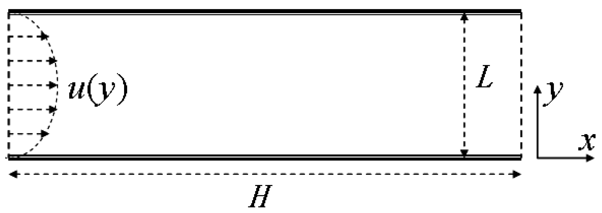
Figure 3.
Comparison of the relative L2-error of and for y at position x = 5 at Wi = 1.0 with and Re = 1.0, respectively.
Figure 3.
Comparison of the relative L2-error of and for y at position x = 5 at Wi = 1.0 with and Re = 1.0, respectively.

Figure 4.
Comparison of the relative L2-error of and for y at position x = 5 at Wi = 15.0 with and Re = 1.0, respectively.
Figure 4.
Comparison of the relative L2-error of and for y at position x = 5 at Wi = 15.0 with and Re = 1.0, respectively.
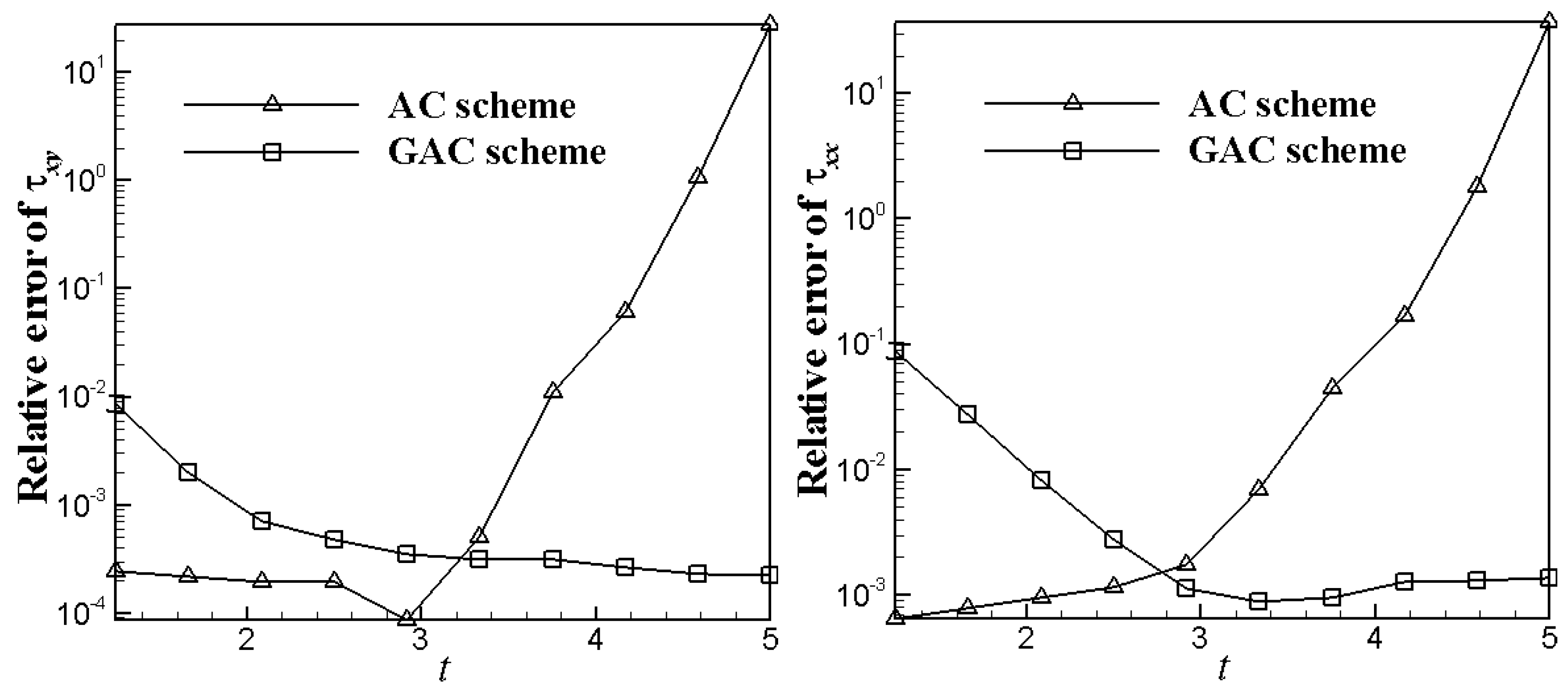
Figure 5.
The time development of the velocity components u at central point (5, 0.5) for Wi = 15.0 (right) with and Re = 1.0, respectively.
Figure 5.
The time development of the velocity components u at central point (5, 0.5) for Wi = 15.0 (right) with and Re = 1.0, respectively.

Figure 6.
A diagram of the planar 4:1 contraction flow.
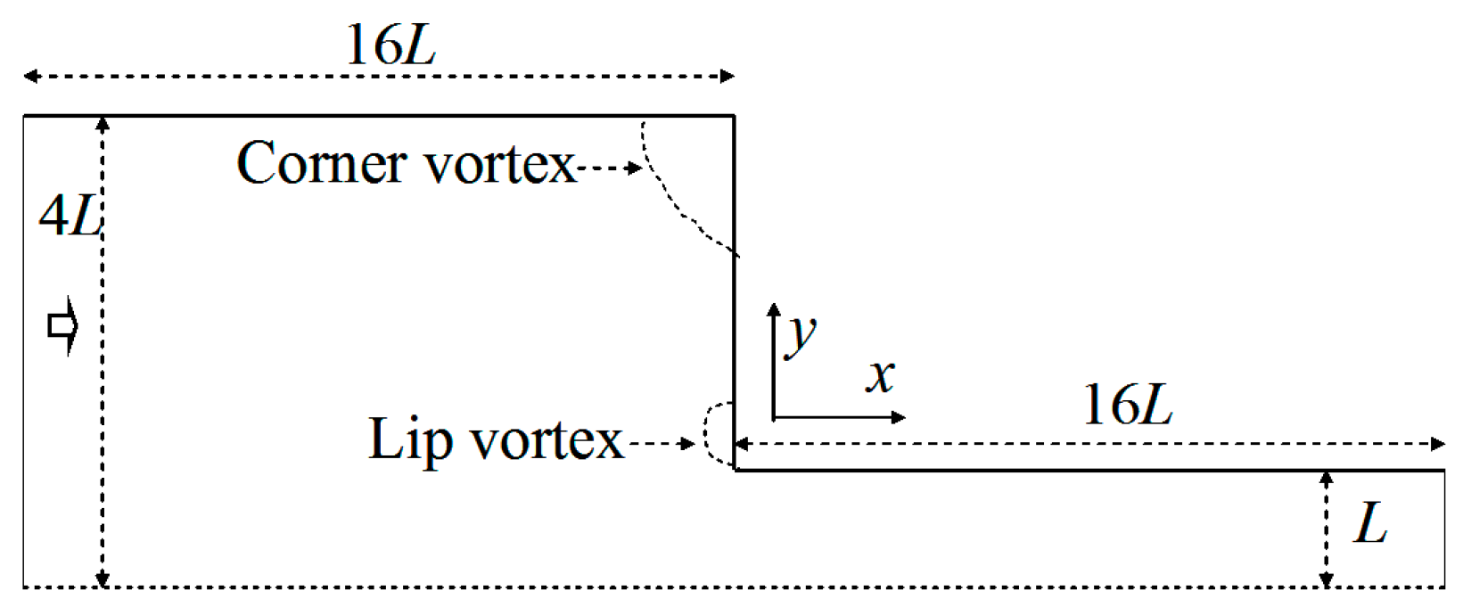
Figure 7.
Mesh dependence of the velocity components through the horizontal at Wi = 1.0 using mesh of M1, M2, and M3.
Figure 7.
Mesh dependence of the velocity components through the horizontal at Wi = 1.0 using mesh of M1, M2, and M3.

Figure 8.
The numerical solutions of velocity components through the horizontal centerlines with Wi = 1.0, comparing between the results of GAC and the AC, respectively.
Figure 8.
The numerical solutions of velocity components through the horizontal centerlines with Wi = 1.0, comparing between the results of GAC and the AC, respectively.
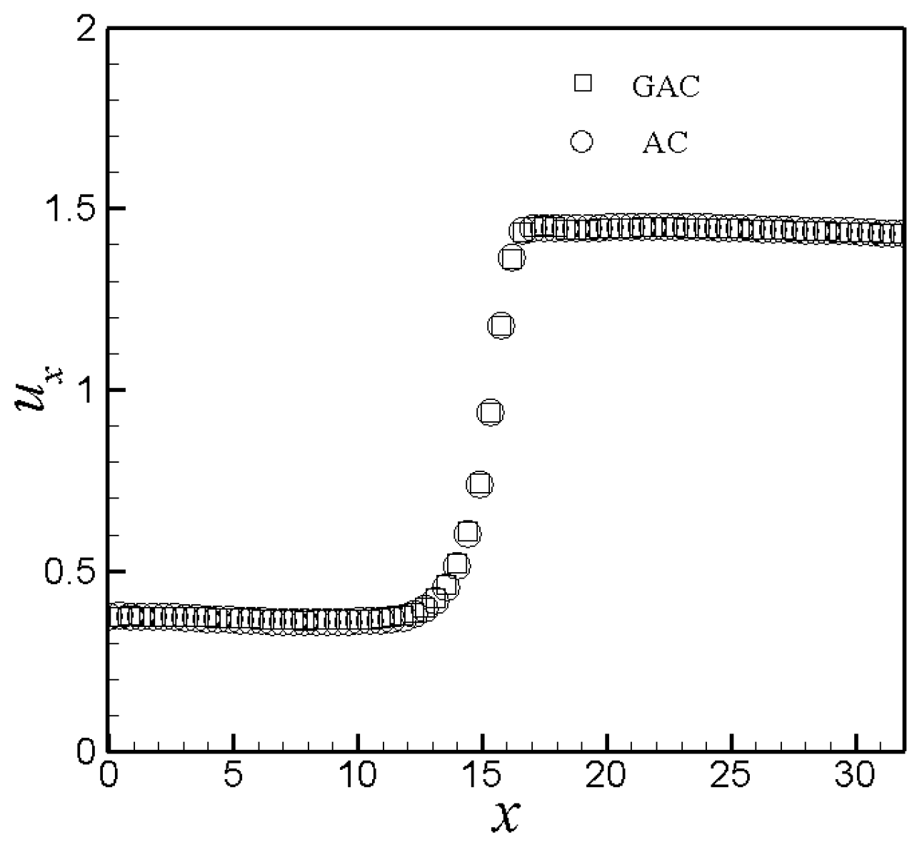
Figure 9.
The instantaneous streamlines of the flow with Wi = 5.0: (a) t = 8, (b) 16, (c) 24, (d) 30.
Figure 9.
The instantaneous streamlines of the flow with Wi = 5.0: (a) t = 8, (b) 16, (c) 24, (d) 30.

Table 1.
Mesh characteristics used in this study.
| Mesh | Total Cell | (x/L) |
|---|---|---|
| M1 | 120,000 | 0.05 |
| M2 | 392,000 | 0.0142 |
| M3 | 512,000 | 0.0125 |
© 2018 by the authors. Licensee MDPI, Basel, Switzerland. This article is an open access article distributed under the terms and conditions of the Creative Commons Attribution (CC BY) license (http://creativecommons.org/licenses/by/4.0/).
Share and Cite
MDPI and ACS Style
Su, J.; Ouyang, J.; Lu, J. A Lattice Boltzmann Method and Asynchronous Model Coupling for Viscoelastic Fluids. Appl. Sci. 2018, 8, 352. https://doi.org/10.3390/app8030352
AMA Style
Su J, Ouyang J, Lu J. A Lattice Boltzmann Method and Asynchronous Model Coupling for Viscoelastic Fluids. Applied Sciences. 2018; 8(3):352. https://doi.org/10.3390/app8030352
Chicago/Turabian StyleSu, Jin, Jie Ouyang, and Junxiang Lu. 2018. "A Lattice Boltzmann Method and Asynchronous Model Coupling for Viscoelastic Fluids" Applied Sciences 8, no. 3: 352. https://doi.org/10.3390/app8030352
Note that from the first issue of 2016, this journal uses article numbers instead of page numbers. See further details here.