Heat Transfer in Non-Newtonian Flows by a Hybrid Immersed Boundary–Lattice Boltzmann and Finite Difference Method


School of Engineering and Information Technology, University of New South Wales, Canberra, ACT 2600, Australia
*
Authors to whom correspondence should be addressed.
Appl. Sci. 2018, 8(4), 559; https://doi.org/10.3390/app8040559
Submission received: 8 March 2018
/
Revised: 2 April 2018
/
Accepted: 3 April 2018
/
Published: 4 April 2018
(This article belongs to the Special Issue Development and Applications of Kinetic Solvers for Complex Flows)
Abstract
:A hybrid immersed boundary–lattice Boltzmann and finite difference method for fluid–structure interaction and heat transfer in non-Newtonian flow is presented. The present numerical method includes four parts: fluid solver, heat transfer solver, structural solver, and immersed boundary method for fluid–structure interaction and heat transfer. Specifically, the multi-relaxation time lattice Boltzmann method is adopted for the dynamics of non-Newtonian flow, with a geometry-adaptive technique to enhance the computational efficiency and immersed boundary method to achieve no-slip boundary conditions. The heat transfer equation is spatially discretized by a second-order up-wind scheme for the convection term, a central difference scheme for the diffusion term, and a second-order difference scheme for the temporal term. The structural dynamics is numerically solved using a finite difference method. The major contribution of this work is the integration of spatial adaptivity, thermal finite difference method, and fluid flow immersed boundary-lattice Boltzmann method. Several benchmark problems including the developing flow of non-Newtonian fluid in a channel, non-Newtonian fluid flow and heat transfer around a stationary cylinder and flow around a stationary cylinder with a detached filament are used to validate the present method and developed solver. The good agreements achieved by the present method with the published data show that the present extension is an efficient way for fluid–structure interaction and heat transfer involving non-Newtonian fluid. The heat transfer around an oscillating cylinder in non-Newtonian fluid flow at Reynolds number of 100 is also numerically studied using the present solver, considering the effects of the oscillating frequency and amplitude. The results may be used to expand the currently limited database of fluid–structure interaction and heat transfer benchmark studies.
1. Introduction
Experiments are expensive and challenging with increasing complexity. As an alternative research method, numerical simulations have attracted much attention in the past twenty years [1]. As an alternative method of computational fluid dynamics (CFD), the lattice Boltzmann method (LBM) has received remarkable attention since its origin [2,3]. After the proposal of the Bhatnagar–Gross–Krook (BGK) collision operator, the efficiency and flexibility of the LBM have been enhanced significantly. Consequently, the BGK-based LBM has been successfully applied to various fluid dynamics problems, such as multiphase flow [4,5,6,7], complex flow in porous media [8], and non-Newtonian flow [9,10]. To address the numerical instability in single-relaxation-time LBM due to low viscosity, entropic [11,12], two-relaxation-time (TRT), and multi-relaxation-time (MRT) LBM methods have been developed [4]. The major advantages of the LBM are its simplicity, easy implementation, explicit calculations, and intrinsic parallel nature. However, the uniform mesh used in the standard LBM limits its applications in engineering [13]. Many efforts have been made to remove this drawback, including differential type and interpolation type LBM. Grid refinement is another way to retain the simplicity of the LBM and enhance computational efficiency. The mesh is locally refined where high resolution is needed. The multi-block technique proposed by Yu et al. [14] divides the fluid field into several blocks with different mesh sizes. As the mesh is initialized before the computation in this method, the mesh refinement is not involved with the fluid field. Wu and Shu proposed a solution-adaptive refinement scheme, where the refinement procedure is decided by the fluid field [13]. By using the refinement technique, the computational efficiency can be highly enhanced. Fluid–structure interaction (FSI) problems extensively exist in engineering. Thanks to the representation of the forcing term introduced by Guo et al. [15], the involved external or internal force can be considered approximately, which also enables the successful combination of the LBM and the immersed boundary method (IBM) (know as IB-LBM) [16,17,18]. The IB-LBM proved to be an efficient method for FSI and has been applied to various problems successfully [10,19,20,21,22,23,24,25,26].
Non-Newtonian fluid is extensively involved in many industrial substances, i.e., blood flow, polymer, and melt solutions. The high viscosity levels in conjunction with the complexity in the behaviour of the stress terms of momentum equations for non-Newtonian fluids generally give rise to the limitation of fluid processing under laminar flow conditions [27,28]. Due to the potential of rheological characteristics (shear-thinning, shear-thickening, etc.) in the applications of engineering, remarkable efforts have been made to develop efficient numerical methods to handle non-Newtonian flows and heat transfer over the last few decades [9,27,29]. As the LBM has proven to be an efficient method for CFD [3], it is thought to be a good idea to employ the LBM to handle non-Newtonian flow and heat transfer. In terms of the simulation of thermal fluid systems, most of the previous thermal LBM models adopt the multi-speed approach [30,31,32], in which additional particle speeds are needed to obtain the energy equation at the macroscopic level [33]. The additional particle speeds decrease the computational efficiency; the stability is also limited. In order to keep the simplicity property of the LBM, Peng et al. proposed a simplified thermal LBM, neglecting the compression work done by the pressure and viscous heat dissipation [34]. In this study, an alternative method to solve the heat transfer in non-Newtonian fluid flow is presented, conserving the simplicity and efficiency of the LBM. The fluid dynamics and heat transfer are solved by the LBM and finite difference method, respectively, with multi-relaxation time and a geometry-adaptive mesh technique to achieve good stability and computational efficiency. In addition to the thermal process, FSI is also achieved using an penalty immersed boundary method. In conclusion, the present method can handle problems involving FSI with complex boundaries and heat transfer in non-Newtonian fluid flow.
In this paper, a hybrid immersed boundary–lattice Boltzmann and finite difference method for FSI and heat transfer in non-Newtonian flow is presented, with the geometry-adaptive Cartesian mesh technique to enhance the computational efficiency. In this contribution, we present for the first time an integration of spatial adaptivity, thermal finite difference method, and fluid flow IB-LBM. The organization of the present paper is as follows. The numerical method is presented in Section 2. Validations of the developing flow of power-law fluid in a channel, power-law fluid flow and heat transfer around a stationary cylinder are presented in Section 3. Section 4 presents the flow around a stationary cylinder with a detached filament. The numerical simulation of heat transfer around an oscillating cylinder is presented in Section 5. Final conclusions are given in Section 6.
2. Numerical Method
In this paper, the two-dimensional non-Newtonian flow and heat transfer involving complex boundaries are considered, where the LBM is adopted for the fluid solver, the finite difference method is used to solve the heat transfer equation and structural dynamics, and the complex no-slip boundaries are achieved by an IB method. The details of the current method will be given in this section.
2.1. Fluid Solver
In the MRT-based IB-LBM, the evolution equation of the velocity distribution function along the i-th direction at position with BGK approximation is expressed as [35]
where is the time step. The collision operator and , which represent the body force effects on the distribution function, are defined as
where M is a transform matrix for the D2Q9 model (two dimensional with 9 directions) used here, and S is a non-negative diagonal matrix related to the fluid viscosity. The details for the determination of S can be found in [36]. The lattice speed is defined as
where is the lattice spacing. Then, the macro density and momentum are given as follows,
The local equilibrium distribution function and the force term are calculated by
where the weights are given by , for , and for . The sound speed , and is the force acting on the fluid. The relaxation time is related to the kinematic viscosity in the Navier–Stokes equations in terms of . The rheological equation of state for power-law non-Newtonian fluid considered in this paper is defined by [27]
where m is the power-law consistency index, n is the power-law fluid behaviour index, and is the second invariant of the rate of strain tensor. Additionally, the multi-block technique developed by Yu et al. [14] is combined with the geometry-adaptive method to enhance the computational efficiency.
2.2. Heat Transfer Solver
The governing equation for the heat transfer in the fluid is given as [37]
where T is the temperature, and are the specific heat and thermal conductivity coefficient of the fluid, respectively. q is the source term.
The second-order upwind scheme is used to discretize the convection term in Equation (9) explicitly, expressed as
A second-order internal central difference scheme is adopted for the spatial discretization on the boundaries. The subscripts indicate the position.
The diffusion term in Equation (9) is discretized using a second-order explicit scheme, expressed as
and the internal difference scheme is also used for the boundary nodes. All the discretizations of T in the y direction is similar to that in the x direction. In addition, a second-order explicit scheme is used for the temporal discretization. Therefore, the heat transfer solver has a second-order accuracy spatially and temporally, which is consistent with the accuracy of the LBM. The heat transfer equation is also solved on the geometry-adaptive Cartesian mesh that used for the fluid dynamics.
2.3. Structural Solver
The geometrically nonlinear motion for the filament considered here is governed by [38,39,40,41,42,43]
where is the linear density of the filament, s is the Lagrangian coordinate along the length, is the stretching coefficient, is the tensile stress defined by , is the position vector of a point on the filament, is the bending rigidity, and is the hydrodynamic stress exerted by the fluid.
The filament is discretized by initially equally spaced nodal points, and the position of the m-th node at time level n is denoted by . The tensile force at the m-th node is calculated by a finite-difference scheme expressed as
where is the grid spacing, the tension T and tangent vector, , at the segment center, , are both computed using a second-order central difference scheme. The bending force are computed using a finite difference scheme expressed as
where is a Kronecker symbol, defined by when and by when . The details of the schemes can be found in [44].
2.4. The IB Method for Fluid–Structure Interaction and Heat Transfer
The pIB method developed by Kim and Peskin [45] is used to handle the no-slip boundaries between the rigid body and the fluid. The interaction force between the fluid and the structure can be determined by the feedback law [45,46]:
where is the boundary velocity obtained by interpolation at the IB, is the structure velocity, and and are large positive free constants. The force acting on the Lagrange structure from the ambient fluid can be taken as a concentrated force acting on the corresponding nodes; thus, it can be added to the body force in Equation (7). Compared to the sharp-interface method [47,48,49,50], the pIB method is particularly suitable here, since in this approach all the grid points within the computational domain are treated with a unified equation.
The transformation between the Euler and Lagrange variables can be realized by the Dirac delta function. The interpolation of velocity and the spreading of the Lagrange force to the adjacent grid points are expressed as
where is the fluid velocity, is the coordinates of structural nodes, is the coordinates of fluid, s is the arc coordinate, and V is the fluid domain, and is the structure domain.
The position of the filament is updated explicitly by
where is calculated using (17). The internal force density of the filament can be calculated using (14) and (15). The details of the computation of the inertial force defined in (13) can be found in [17]. The can then be calculated by Equation (13). The force acting on the fluid in Equation (18) is the reaction force of defined in Equation (13). Equation (18) is used to distribute the force to the ambient fluid.
The smooth function is used to approximate the Dirac delta function
In this paper, the four-point delta function introduced by Peskin [51] is used
The heat transferred from the immersed boundary to the fluid can be written as [52]
where Q is the virtual boundary heat flux. When the temperature boundary is used, then Q can be calculated using the penalty immersed-boundary method, expressed as
where is a large factor, is the boundary condition on the immersed boundary, and is the temperature of the virtual boundary, interpolated by
3. Validations
3.1. The Developing Flow of Non-Newtonian Power-Law Fluid in a Channel
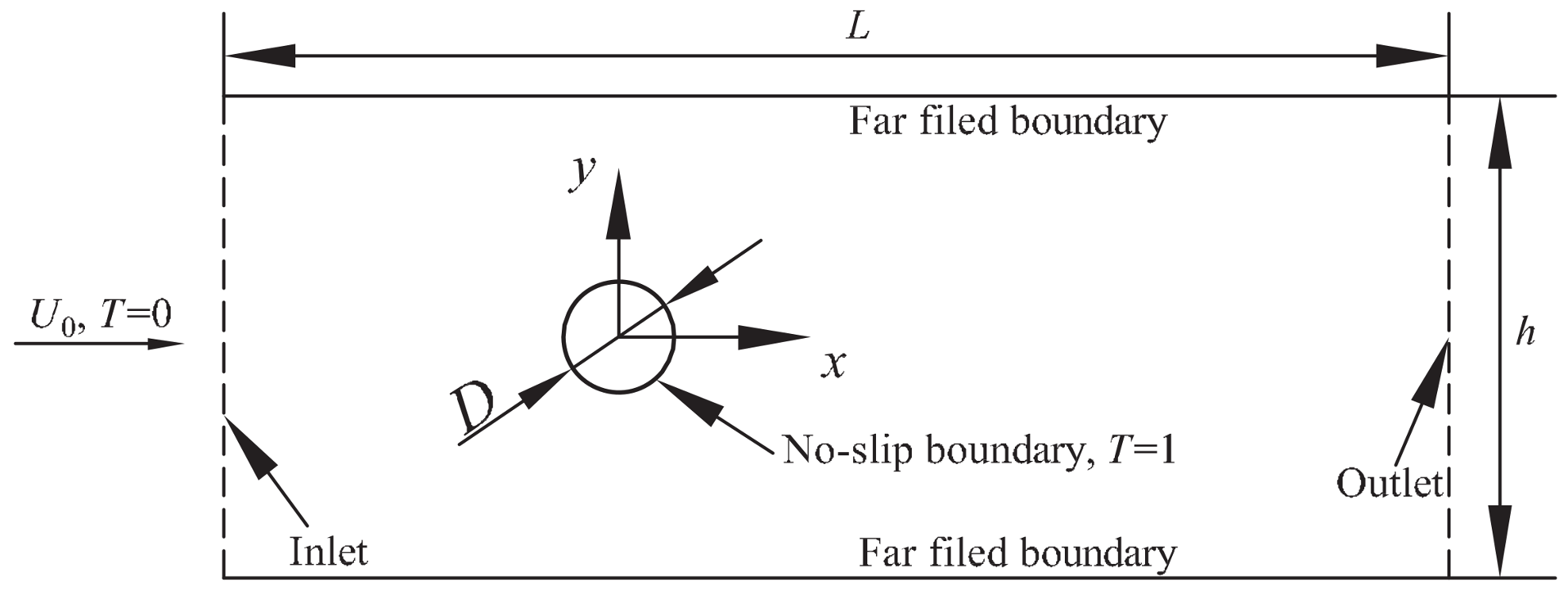
The developing flow through a confined channel has been extensively used as a benchmark validation for non-Newtonian fluid. In this section, the two-dimensional steady laminar developing flow is considered to validate the in-house code. In the numerical simulation, the flow of power-law fluid develops with a uniform inlet velocity () through a rectangular channel of h in height and L in length, as shown in Figure 1. The macro density and velocities on the boundaries are set as at , at and h for the channel wall, and at . The non-equilibrium extrapolation presented by Guo et al. [53] is adopted to calculate the velocity distribution functions on the boundaries.
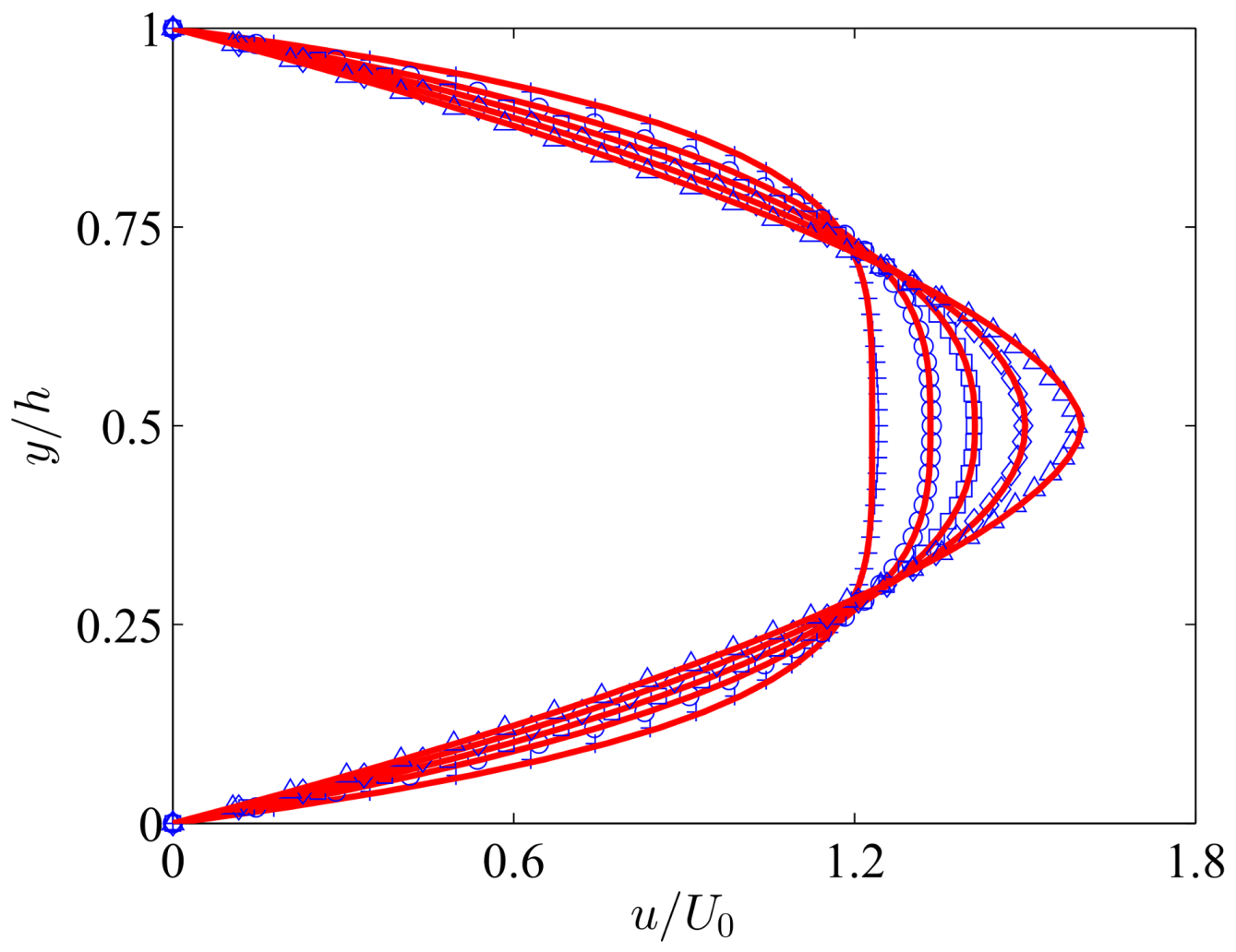
The numerical simulation is performed in a computational domain with the size of and the uniform mesh size is . The dimensionless time step . The Reynolds number (Re) that controls this problem is defined as Re = . The Reynolds number of 10 is used in the current steady simulation, and five power-law indexes n ranging from to (including shear-thinning , shear-thickening , and Newtonian fluid ) are considered. The analytical solution of the velocity profiles of the fully developed flow can be expressed as [27]
The fully developed velocity profiles from present numerical simulations and that predicted by Equation (25) are presented in Figure 2. According to the comparisons in Figure 2, excellent agreements (discrepancies ) are achieved by the present numerical method. The velocity peaks presented in Table 1 also show the good accuracy of the current method.
3.2. Non-Newtonian Power-Law Fluid Flow and Heat Transfer around a Stationary Cylinder
Non-Newtonian power-law fluid flow and heat transfer from a stationary cylinder is considered to validate the accuracy of the present numerical method in handling FSI and heat transfer. The two-dimensional power-law fluid inlets with a uniform flow over a stationary circular cylinder (of diameter D), with the computational domain extending from to , as shown in Figure 3.
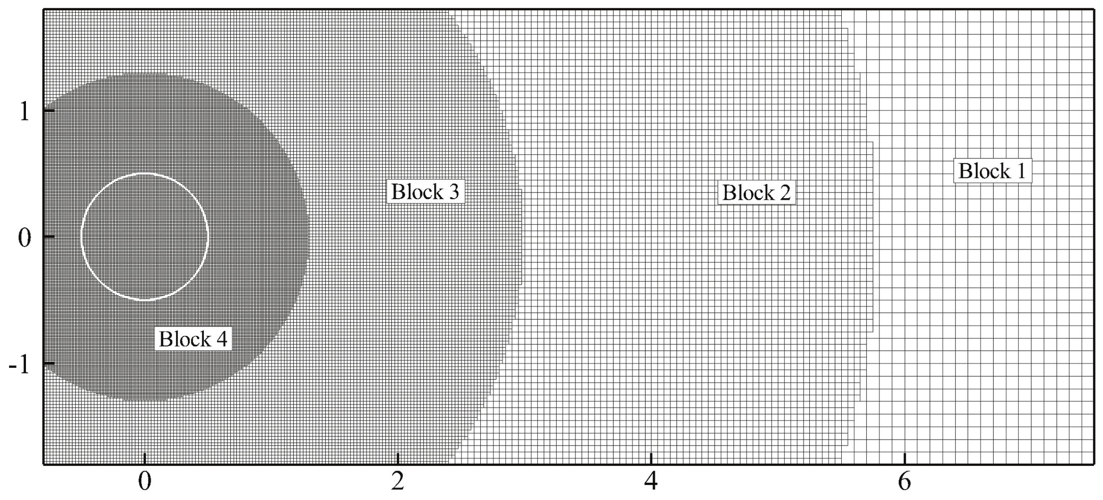
In order to improve the computational efficiency and validate the geometry-adaptive technique utilized in present in-house code, four blocks are used in the simulations, as shown in Figure 4, and the most refined mesh size of the fluid domain is . The dimensionless time step .
The non-dimensional parameters that control this problem include the Reynolds number (Re) and the Prandtl number (Pr), which are defined as
The drag coefficient, lift coefficient, and Strouhal number are defined as
where T is the vortex shedding period, and and are the horizontal and vertical components of acting on the cylinder calculated by Equation (16).
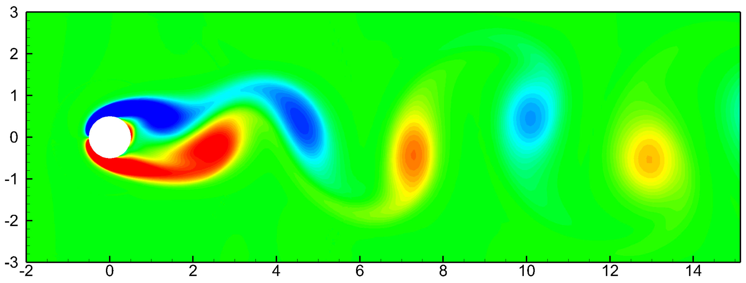
Firstly, we consider the unsteady flow of non-Newtonian power-law flow over a cylinder at Re (at which the flow patterns show von-Kármán periodic vortex shedding behind the cylinder) to validate the geometry-adaptive fluid solver in terms of handling FSI problem. In order to achieve the early von-Kármán vortex shedding, a vertical velocity perturbation is introduced into the initial inlet boundary. Four different indexes , , and are calculated. Table 2 shows the present results of St, (mean drag coefficient) and as well as results from the literature. It shows that the present results agree well with these other values. A snapshot of the vortex contour for Re = 100 and after periodic shedding are presented in Figure 5.
After the validation of the fluid solver in computing FSI problems involving non-Newtonian flow, we further consider the steady flow and heat transfer around a cylinder. The average Nusselt number () used for quantitative comparison with the available data from the literature are defined as
where is the local Nusselt number on the surface of the cylinder, it can be evaluated using the temperature field according to
where is the unit vector normal to the surface of the cylinder.
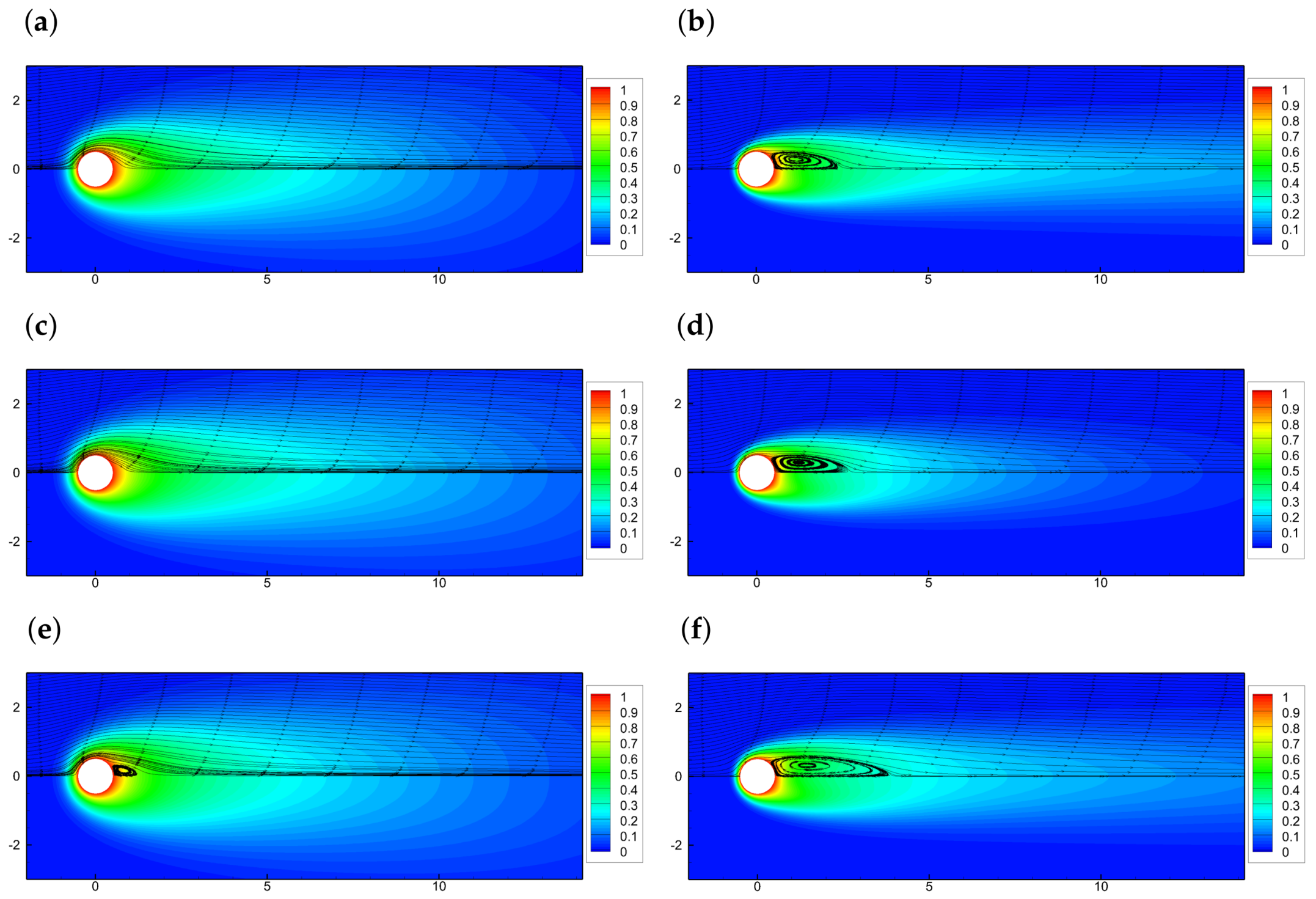
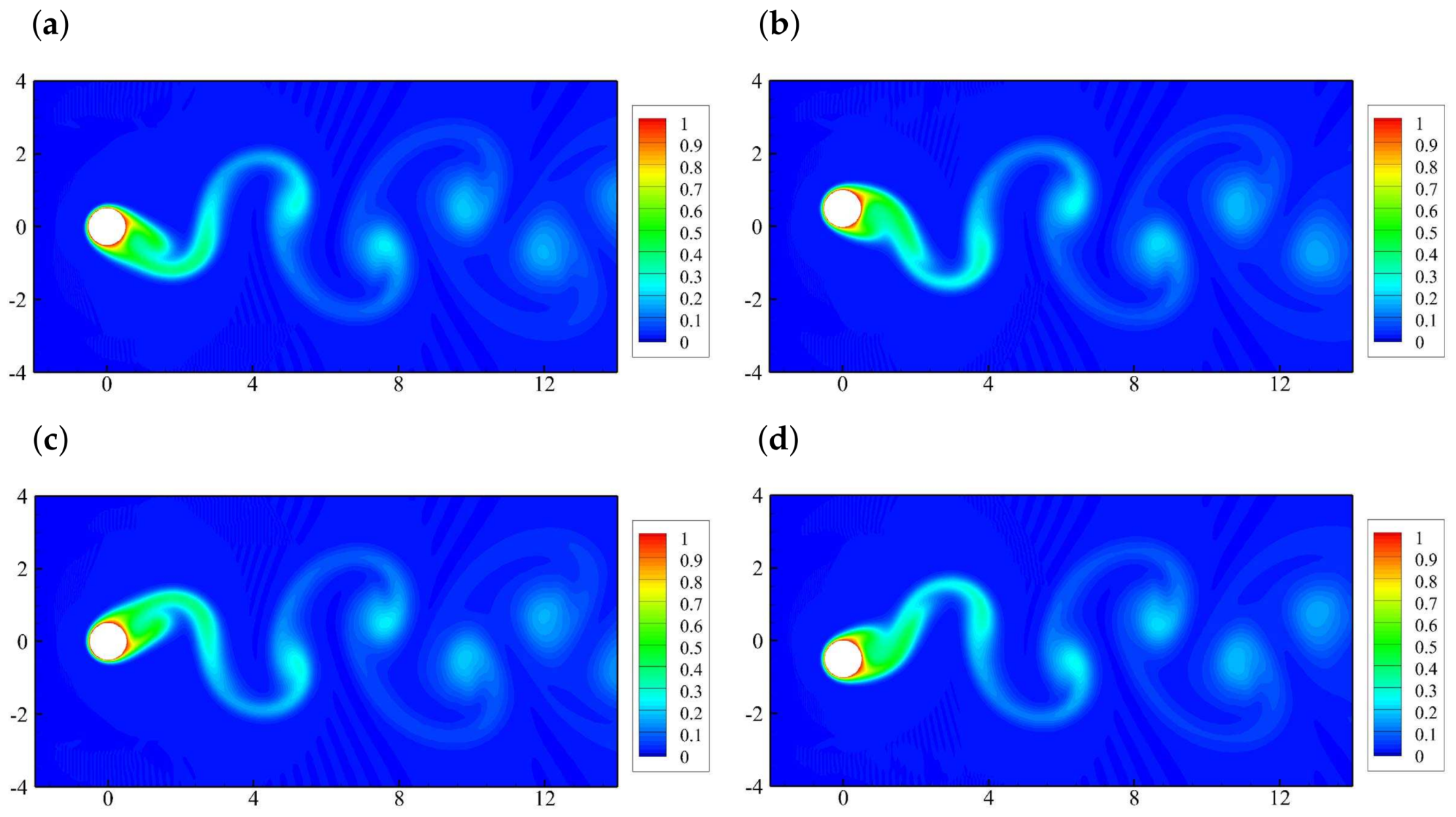
The average Nusselt number from the current computation along with the available data from the literature of two Reynolds number (Re = 10 and 40) and three indexes (, , and ) are presented in Table 3. It is found that the present results are in good agreement with other published data. With the increase of n from to , the average Nusselt number decreases slightly at both Reynolds numbers. Comparisons between the Reynolds numbers of 10 and 40 show that the average Nusselt number changes more remarkably with larger Reynolds numbers. It is because of the enhancement of the heat convection effects under the larger Reynolds number. The snapshots of the temperature field from current simulations are presented in Figure 6. As is readily seen from Figure 6, the length of the vortex attached behind the cylinder stretches significantly with n increasing from 0.8 to 1.4, which also qualitatively agrees with the analysis in [54].
4. Heat Transfer around a Stationary Cylinder with a Detached Filament
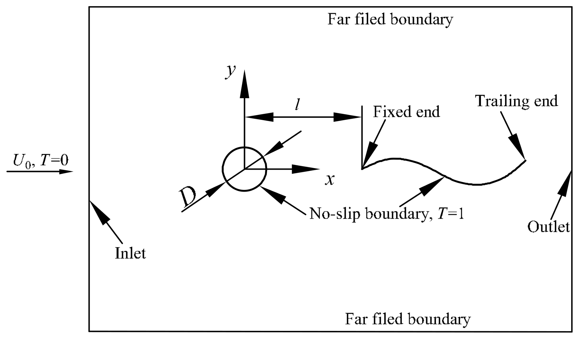
A stationary cylinder with a detached flexible filament is considered in this section, as shown in Figure 7, where D is the diameter of the fixed cylinder, L is the length of the filament, and l is the distance from the origin of the cylinder to the fixed end of the filament. This model has been extensively used to study fish behaviors in a street wake [17,59,60,61]. Simulations are performed at , , and Re = 100. The non-dimensional stretching coefficient defined by is 1000 (the filament is approximately inextensible), and the non-dimensional bending rigidity defined by is . The mesh size around the cylinder and filament is D/160. The dimensionless time step . Three power-law indices , , and , and two filament lengths and are considered.
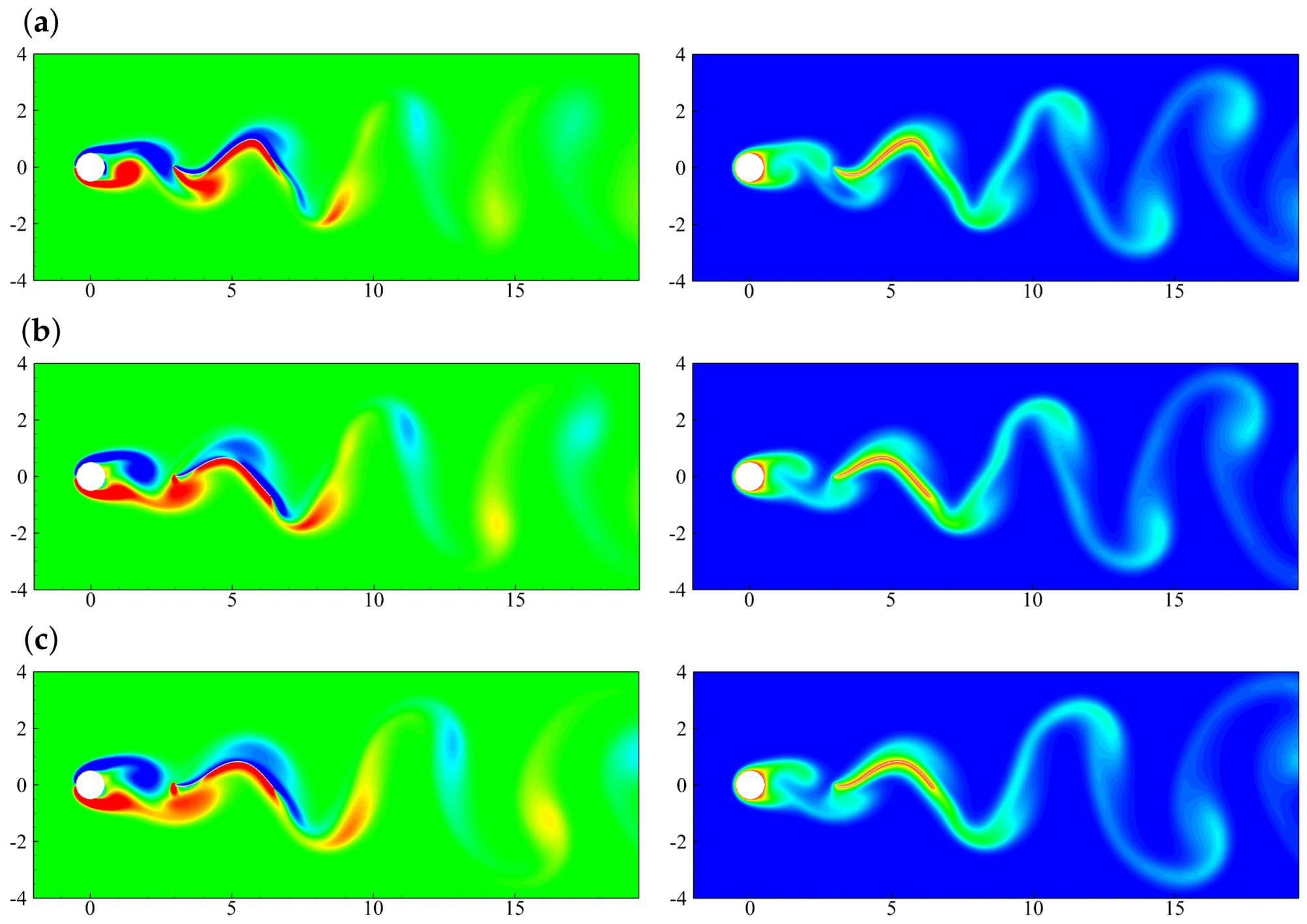
The averaged drag coefficient (), the Strouhal number (), the averaged Nusselt number () of the cylinder, and the vertical flapping amplitude () of the trailing end of the filament are presented in Table 4. The good agreements of the drag coefficient, Strouhal number, and flapping amplitude between the present results and the data from [17,60] show the excellent accuracy of the present solver. The longer filament generates a larger flapping amplitude, but the filament length does not significantly affect other fluid and temperature characteristics, as shown in Table 4. The results from non-Newtonian fluid flow show that the shear-thickening fluid generates larger drag comparing with shear-thinning fluid, but presents an opposite tendency, as analysed in Section 3.2. Additionally, the current results show that the power index does not have significant influence on the flapping amplitude. The instantaneous vortex and temperature contours are presented in Figure 8. The non-Newtonian results presented here can be used to extend the limited database involving FSI.
5. Heat Transfer around an Oscillating Cylinder in Non-Newtonian Fluid Flow
5.1. Physical Problem
In this section, the heat transfer around an oscillating cylinder in non-Newtonian fluid flow is considered, which can be taken as validations for heat transfer involving moving boundaries in the future. In this problem, the center of the cylinder undergoes a translational motion governed by
where and f are the oscillating amplitude and frequency, respectively. The non-dimensional parameters governing this problem including oscillating frequency and amplitude can be written as
The Reynolds number and Prantdl number are defined as those in Equation (26). In the current simulation, the influences of the oscillating amplitude, frequency, and power index are considered.
5.2. Effects of the Oscillating Amplitude
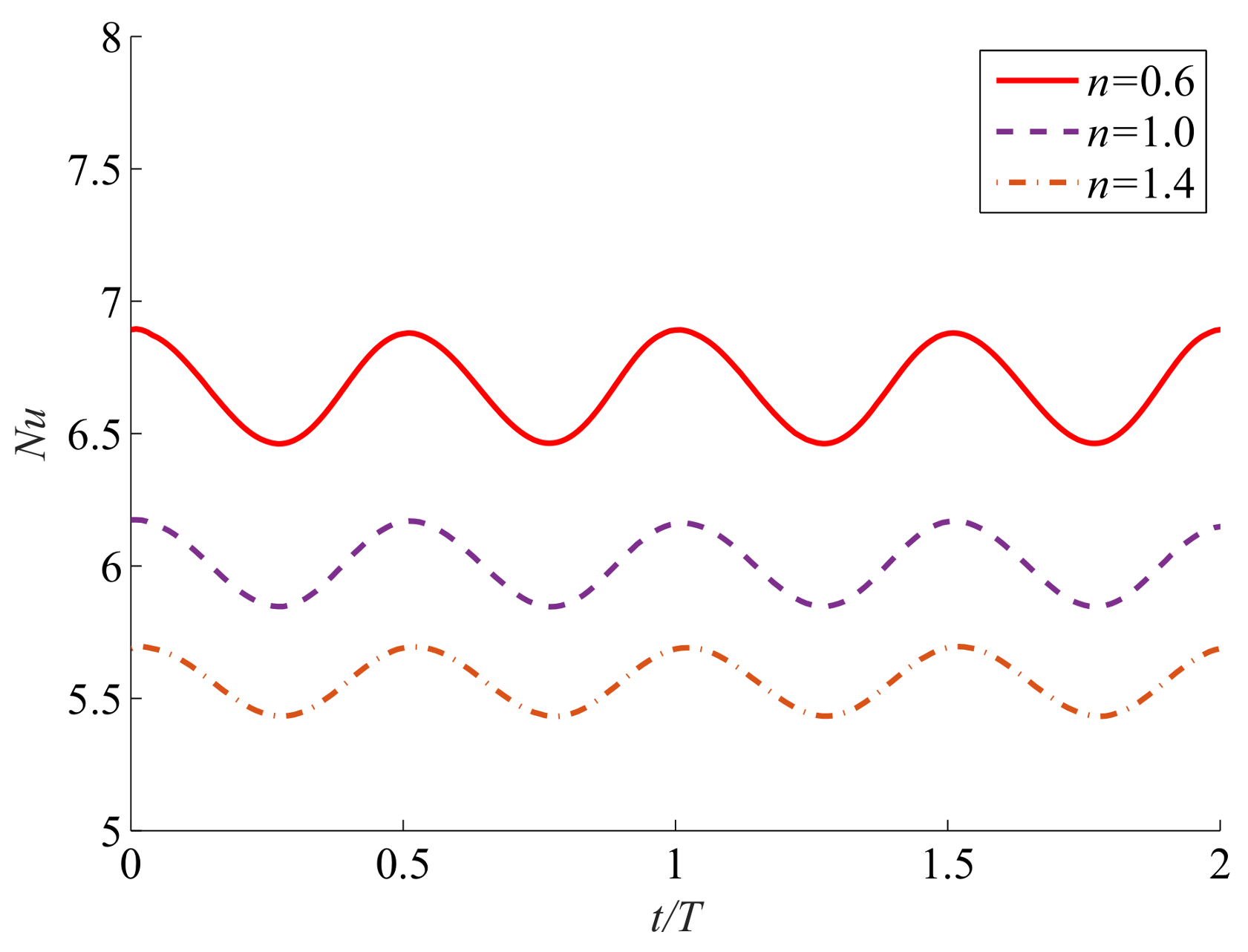
In the current simulations, the cylinder oscillates in the frequency of the vortex shedding, so the value of the non-dimensional oscillating frequency () is 1.0. The Reynolds number and the Prantdl number defined in Equation (26) are 100 and 1.0, respectively. Three indexes (, and 1.4) are numerically computed to include shear-thinning, Newtonian, and shear-thickening fluid. The Strouhal numbers defined in Equation (27) for these cases have already been given in Table 2 above. Three non-dimensional oscillating amplitudes () , , and are considered to identify the effects of the amplitude. The time-averaged Nusselt numbers and their amplitudes () from the present computations are presented in Table 5, where the amplitudes for are negligible (less than 1.0%) and thus not presented. The results show that the time-averaged Nusselt number is much higher in the shear-thinning () fluid than in the shear-thickening () fluid, which agrees with that in the previous steady cases. It also shows that the increasing oscillating amplitude enhances the heat convection effects, and the oscillation of the averaged Nusselt number tends to be more remarkable with increasing . Figure 9 presents time histories of the averaged Nusselt numbers for in two periods. The averaged Nusselt number has a frequency of . The snapshots of the temperature fields for and in a period are further presented in Figure 10.
5.3. Effects of the Oscillating Frequency
Here, in order to study the effects of the oscillating frequency on the heat transfer around an oscillating cylinder in a uniform flow, the oscillating amplitude is fixed at with Re = 100. Two more oscillating frequencies and are considered for comparison. The time-averaged Nusselt numbers and amplitudes are presented in Table 6. The results show that the increasing oscillating frequency of the cylinder enhances the heat convection, resulting in larger averaged Nusselt numbers and amplitudes for both shear-thinning and shear-thickening fluids. However, the enhancement in the shear-thinning fluid is much more significant than that in the shear-thickening fluid.
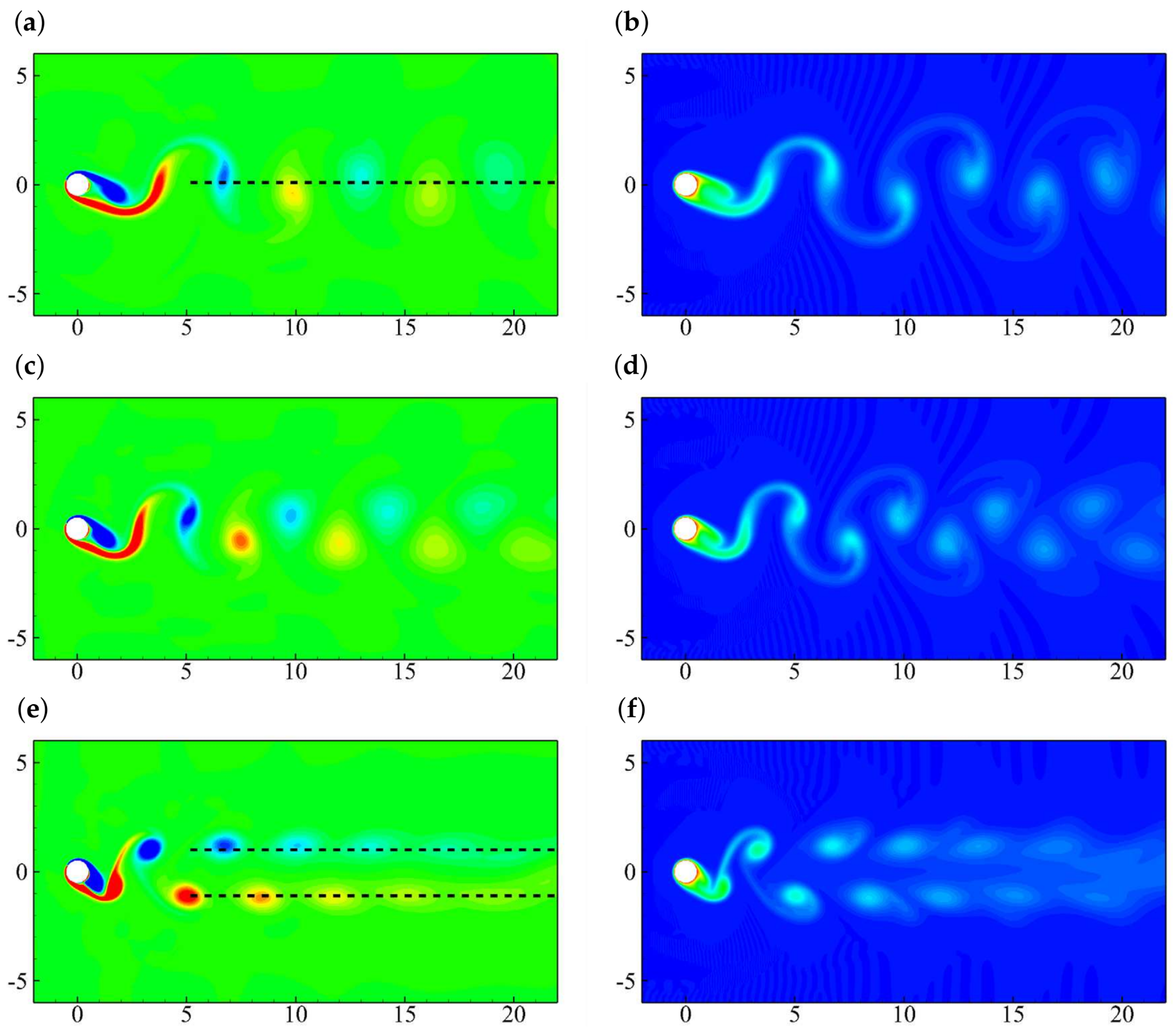
The instantaneous vorticity and temperature contours for are presented in Figure 11. Similar Kármán-street type wake is observed in all cases. It is found that the increasing oscillating frequency of the cylinder tends to increase the vertical distance between the two adjacent vortices. Specifically, the vortices shed at are almost in a line (as marked in Figure 11a) as oscillating frequency increases, and the vortices tend to separate vertically (as marked in Figure 11c). The temperature contours show that the heat transfer in the fluid exactly follows these vortices.
6. Conclusions
In this paper, a hybrid immersed boundary–lattice Boltzmann and finite difference method for fluid–structure interaction and heat transfer in non-Newtonian flow is presented, with the geometry-adaptive Cartesian mesh technique to enhance the computational efficiency. The present numerical method includes four parts: the fluid solver, heat transfer solver, structural solver, and immersed boundary method for fluid–structure interaction and heat transfer. Specifically, the multi-relaxation-time-based LBM is adopted for the computation of non-Newtonian flow, with the geometry-adaptive Cartesian mesh technique to enhance the computational efficiency. The heat transfer equation is spatially discretized by a second-order up-wind scheme for the convection term, a central difference scheme for the diffusion term, and a second-order difference scheme for the temporal term. The structural dynamics is numerically solved using a finite difference method. The no-slip boundary is achieved using an immersed boundary method.
The proposed method and developed solver is validated with standard benchmark problems involving the non-Newtonian fluids flow, i.e., the developing flow of non-Newtonian fluid in a channel, heat transfer around a stationary cylinder and flow around a stationary cylinder with a detached filament. The good agreements achieved by the present method with the published data show that the present extension is an efficient way for fluid–structure interaction and heat transfer involving non-Newtonian fluid.
The heat transfer around an oscillating cylinder in non-Newtonian fluid flow is also numerically studied using the present method, considering the effects of the oscillating frequency and amplitude. The results show that the increasing frequency and amplitude tend to enhance the heat convection, resulting in larger time-averaged Nusselt numbers. The enhancement that occurs in the shear-thinning fluid is much more significant than that in the shear-thickening fluid. The present results may be used to expand the currently limited database of FSI and heat transfer benchmark studies.
Acknowledgments
F.-B.T. is the recipient of an Australian Research Council Discovery Early Career Researcher Award (project number DE160101098).
Author Contributions
L.W. and F.-B.T. conceived the ideal. L.W. developed the code and conducted the simulation. L.W. and F.-B.T. analysed the results, drafted and revised the manuscript.
Conflicts of Interest
The authors declare no conflict of interest.
Abbreviations
The following abbreviations are used in this manuscript:
| CFD | computational fluid dynamics |
| LBM | lattice Boltzmann method |
| IBM | immersed boundary method |
| BGK | Bhatnagar-Gross-Krook |
| TRT | two-relaxation time |
| MRT | multi-relaxation time |
| FSI | fluid–structure interaction |
References
- Bazilevs, Y.; Takizawa, K.; Tezduyar, T.E. Computational Fluid-Structure Interaction: Methods and Applications; John Wiley & Sons: New York, NY, USA, 2013. [Google Scholar]
- Chen, S.; Doolen, G.D. Lattice Boltzmann method for fluid flows. Annu. Rev. Fluid Mech. 1998, 30, 329–364. [Google Scholar] [CrossRef]
- Guo, Z.; Shu, C. Lattice Boltzmann Method and Its Applications in Engineering; World Scientific: Singapore, 2013. [Google Scholar]
- McCracken, M.E.; Abraham, J. Multiple-relaxation-time lattice-Boltzmann model for multiphase flow. Phys. Rev. E 2005, 71, 036701. [Google Scholar] [CrossRef] [PubMed]
- Zheng, H.; Shu, C.; Chew, Y.-T. A lattice Boltzmann model for multiphase flows with large density ratio. J. Comput. Phys. 2006, 218, 353–371. [Google Scholar] [CrossRef]
- Wang, Y.; Shu, C.; Huang, H.; Teo, C. Multiphase lattice Boltzmann flux solver for incompressible multiphase flows with large density ratio. J. Comput. Phys. 2015, 280, 404–423. [Google Scholar] [CrossRef]
- Wang, Y.; Shu, C.; Yang, L. An improved multiphase lattice Boltzmann flux solver for three-dimensional flows with large density ratio and high reynolds number. J. Comput. Phys. 2015, 302, 41–58. [Google Scholar] [CrossRef]
- Spaid, M.A.; Phelan, F.R., Jr. Lattice Boltzmann methods for modeling microscale flow in fibrous porous media. Phys. Fluids 1997, 9, 2468–2474. [Google Scholar] [CrossRef]
- Gabbanelli, S.; Drazer, G.; Koplik, J. Lattice Boltzmann method for non-newtonian (power-law) fluids. Phys. Rev. E 2005, 72, 046312. [Google Scholar] [CrossRef] [PubMed]
- Tian, F.-B. Deformation of a capsule in a power-law shear flow. Comput. Math. Methods Med. 2016, 2016, 7981386. [Google Scholar] [CrossRef] [PubMed]
- Boghosian, B.M.; Yepez, J.; Coveney, P.V.; Wager, A. Entropic lattice Boltzmann methods. Proc. R. Soc. Lond. A Math. Phys. Eng. Sci. 2001, 457, 717–766. [Google Scholar] [CrossRef]
- Ansumali, S.; Karlin, I.V. Single relaxation time model for entropic lattice Boltzmann methods. Phys. Rev. E 2002, 65, 056312. [Google Scholar] [CrossRef] [PubMed]
- Wu, J.; Shu, C. A solution-adaptive lattice Boltzmann method for two-dimensional incompressible viscous flows. J. Comput. Phys. 2011, 230, 2246–2269. [Google Scholar] [CrossRef]
- Yu, D.; Mei, R.; Shyy, W. A multi-block lattice Boltzmann method for viscous fluid flows. Int. J. Numer. Methods Fluids 2002, 39, 99–120. [Google Scholar] [CrossRef]
- Guo, Z.; Zheng, C.; Shi, B. Discrete lattice effects on the forcing term in the lattice Boltzmann method. Phys. Rev. E 2002, 65, 046308. [Google Scholar] [CrossRef] [PubMed]
- Feng, Z.-G.; Michaelides, E.E. The immersed boundary-lattice Boltzmann method for solving fluid–particles interaction problems. J. Comput. Phys. 2004, 195, 602–628. [Google Scholar] [CrossRef]
- Tian, F.-B.; Luo, H.; Zhu, L.; Liao, J.C.; Lu, X.-Y. An efficient immersed boundary-lattice Boltzmann method for the hydrodynamic interaction of elastic filaments. J. Comput. Phys. 2011, 230, 7266–7283. [Google Scholar] [CrossRef] [PubMed]
- Wang, Y.; Shu, C.; Teo, C.; Wu, J. An immersed boundary-lattice Boltzmann flux solver and its applications to fluid–structure interaction problems. J. Fluids Struct. 2015, 54, 440–465. [Google Scholar] [CrossRef]
- Wu, J.; Shu, C. Implicit velocity correction-based immersed boundary-lattice Boltzmann method and its applications. J. Comput. Phys. 2009, 228, 1963–1979. [Google Scholar] [CrossRef]
- Shu, C.; Liu, N.; Chew, Y.-T. A novel immersed boundary velocity correction–lattice Boltzmann method and its application to simulate flow past a circular cylinder. J. Comput. Phys. 2007, 226, 1607–1622. [Google Scholar] [CrossRef]
- Zhang, J.; Johnson, P.C.; Popel, A.S. An immersed boundary lattice Boltzmann approach to simulate deformable liquid capsules and its application to microscopic blood flows. Phys. Biol. 2007, 4, 285. [Google Scholar] [CrossRef] [PubMed]
- Tian, F.-B.; Luo, H.; Zhu, L.; Lu, X.Y. Interaction between a flexible filament and a downstream rigid body. Phys. Rev. E 2010, 82, 026301. [Google Scholar] [CrossRef] [PubMed]
- Xu, Y.Q.; Tian, F.B.; Li, H.; Deng, Y. Red blood cell partitioning and blood flux redistribution in microvascular bifurcation. Theor. Appl. Mech. Lett. 2012, 2, 024001. [Google Scholar] [CrossRef]
- Xu, Y.Q.; Tian, F.B.; Deng, Y.L. An efficient red blood cell model in the frame of IB–LBM and its application. Int. J. Biomath. 2013, 6, 1250061. [Google Scholar] [CrossRef]
- Liu, Z.; Lai, J.C.; Young, J.; Tian, F.B. Discrete vortex method with flow separation corrections for flapping-foil power generators. AIAA J. 2016, 55, 410–418. [Google Scholar] [CrossRef]
- Liu, Z.; Tian, F.B.; Lai, J.C.; Young, J. Flapping foil power generator performance enhanced with a spring-connected tail. Phys. Fluids 2017, 29, 123601. [Google Scholar] [CrossRef]
- Tian, F.-B.; Bharti, R.P.; Xu, Y.-Q. Deforming-spatial-domain/stabilized space–time (DSD/SST) method in computation of non-newtonian fluid flow and heat transfer with moving boundaries. Comput. Mech. 2014, 53, 257–271. [Google Scholar] [CrossRef]
- Tian, F.-B.; Zhu, L.; Fok, P.W.; Lu, X.Y. Simulation of a pulsatile non-Newtonian flow past a stenosed 2D artery with atherosclerosis. Comput. Biol. Med. 2013, 53, 1098–1113. [Google Scholar] [CrossRef] [PubMed]
- Behr, M.A.; Franca, L.P.; Tezduyar, T.E. Stabilized finite element methods for the velocity-pressure-stress formulation of incompressible flows. Comput. Methods Appl. Mech. Eng. 1993, 104, 31–48. [Google Scholar] [CrossRef]
- Alexander, F.J.; Chen, S.; Sterling, J. Lattice Boltzmann thermohydrodynamics. Phys. Rev. E 1993, 47, R2249. [Google Scholar] [CrossRef]
- Qian, Y. Simulating thermohydrodynamics with lattice BGK models. J. Sci. Comput. 1993, 8, 231–242. [Google Scholar] [CrossRef]
- Chen, Y.; Ohashi, H.; Akiyama, M. Two-parameter thermal lattice BGK model with a controllable prandtl number. J. Sci. Comput. 1997, 12, 169–185. [Google Scholar] [CrossRef]
- Inamuro, T.; Yoshino, M.; Inoue, H.; Mizuno, R.; Ogino, F. A lattice Boltzmann method for a binary miscible fluid mixture and its application to a heat-transfer problem. J. Comput. Phys. 2002, 179, 201–215. [Google Scholar] [CrossRef]
- Peng, Y.; Shu, C.; Chew, Y. Simplified thermal lattice Boltzmann model for incompressible thermal flows. Phys. Rev. E 2003, 68, 026701. [Google Scholar] [CrossRef] [PubMed]
- Guo, Z.; Zheng, C. Analysis of lattice Boltzmann equation for microscale gas flows: Relaxation times, boundary conditions and the knudsen layer. Int. J. Comput. Fluid Dyn. 2008, 22, 465–473. [Google Scholar] [CrossRef]
- Peng, Y.; Shu, C.; Chew, Y.; Niu, X.; Lu, X. Application of multi-block approach in the immersed boundary–lattice Boltzmann method for viscous fluid flows. J. Comput. Phys. 2006, 218, 460–478. [Google Scholar] [CrossRef]
- Abel, S.; Prasad, K.; Mahaboob, A. Buoyancy force and thermal radiation effects in MHD boundary layer visco-elastic fluid flow over continuously moving stretching surface. Int. J. Therm. Sci. 2005, 44, 465–476. [Google Scholar] [CrossRef]
- Wu, J.; Shu, C.; Zhao, N.; Tian, F.B. Numerical study on the power extraction performance of a flapping foil with a flexible tail. Phys. Fluids 2015, 27, 013602. [Google Scholar] [CrossRef]
- Tian, F.B.; Wang, Y.; Young, J.; Lai, J.C. An FSI solution technique based on the DSD/SST method and its applications. Math. Models Methods Appl. Sci. 2015, 25, 2257–2285. [Google Scholar] [CrossRef]
- Tian, F.B. FSI modeling with the DSD/SST method for the fluid and finite difference method for the structure. Comput. Mech. 2014, 54, 581–589. [Google Scholar] [CrossRef]
- Wu, J.; Wu, J.; Tian, F.B.; Zhao, N.; Li, Y.D. How a flexible tail improves the power extraction efficiency of a semi-activated flapping foil system: A numerical study. J. Fluids Struct. 2015, 54, 886–899. [Google Scholar] [CrossRef]
- Tian, F.B.; Young, J.; Lai, J.C.S. Improving power-extraction efficiency of a flapping plate: From passive deformation to active control. J. Fluids Struct. 2014, 51, 384–392. [Google Scholar] [CrossRef]
- Tian, F.B.; Luo, H.; Song, J.; Lu, X.Y. Force production and asymmetric deformation of a flexible flapping wing in forward flight. J. Fluids Struct. 2013, 36, 149–161. [Google Scholar] [CrossRef]
- Zhu, L.; Peskin, C.S. Simulation of a flapping flexible filament in a flowing soap film by the immersed boundary method. J. Comput. Phys. 2002, 179, 452–468. [Google Scholar] [CrossRef]
- Kim, Y.; Peskin, C.S. Penalty immersed boundary method for an elastic boundary with mass. Phys. Fluids 2007, 19, 053103. [Google Scholar] [CrossRef]
- Deng, H.B.; Chen, D.D.; Dai, H.; Wu, J.; Tian, F.B. On numerical modeling of animal swimming and flight. Comput. Mech. 2013, 52, 1221–1242. [Google Scholar] [CrossRef]
- Tian, F.-B.; Dai, H.; Luo, H.; Doyle, J.F.; Rousseau, B. Fluid–structure interaction involving large deformations: 3D simulations and applications to biological systems. J. Comput. Phys. 2014, 258, 451–469. [Google Scholar] [CrossRef] [PubMed]
- Tian, F.-B.; Lu, X.Y.; Luo, H. Onset of instability of a flag in uniform flow. Theor. Appl. Mech. Lett. 2012, 2, 022005. [Google Scholar] [CrossRef]
- Shahzad, A.; Tian, F.B.; Young, J.; Lai, J.C.S. Effects of wing shape, aspect ratio and deviation angle on aerodynamic performance of flapping wings in hover. Phys. Fluids 2016, 28, 111901. [Google Scholar] [CrossRef]
- Mittal, R.; Dong, H.; Bozkurttas, M.; Najjar, F.M.; Vargas, A.; von Loebbecke, A. A versatile sharp interface immersed boundary method for incompressible flows with complex boundaries. J. Comput. Phys. 2008, 227, 4825–4852. [Google Scholar] [CrossRef] [PubMed]
- Peskin, C.S. The immersed boundary method. Acta Numer. 2002, 11, 479–517. [Google Scholar] [CrossRef]
- Ren, W.; Shu, C.; Wu, J.; Yang, W. Boundary condition-enforced immersed boundary method for thermal flow problems with dirichlet temperature condition and its applications. Comput. Fluids 2012, 57, 40–51. [Google Scholar] [CrossRef]
- Guo, Z.; Zheng, C.; Shi, B. An extrapolation method for boundary conditions in lattice Boltzmann method. Phys. Fluids 2002, 14, 2007–2010. [Google Scholar] [CrossRef]
- Patnana, V.K.; Bharti, R.P.; Chhabra, R.P. Two-dimensional unsteady flow of power-law fluids over a cylinder. Chem. Eng. Sci. 2009, 64, 2978–2999. [Google Scholar] [CrossRef]
- Wang, L.; Currao, G.M.; Han, F.; Neely, A.J.; Young, J.; Tian, F.-B. An immersed boundary method for fluid–structure interaction with compressible multiphase flows. J. Comput. Phys. 2017, 341, 131–151. [Google Scholar] [CrossRef]
- Xu, S.; Wang, Z.J. An immersed interface method for simulating the interaction of a fluid with moving boundaries. J. Comput. Phys. 2006, 216, 454–493. [Google Scholar] [CrossRef]
- Bharti, R.; Sivakumar, P.; Chhabra, R. Forced convection heat transfer from an elliptical cylinder to power-law fluids. Int. J. Heat Mass Transf. 2008, 51, 1838–1853. [Google Scholar] [CrossRef]
- Soares, A.; Ferreira, J.; Chhabra, R. Flow and forced convection heat transfer in crossflow of non-newtonian fluids over a circular cylinder. Ind. Eng. Chem. Res. 2005, 44, 5815–5827. [Google Scholar] [CrossRef]
- Alben, S. Simulating the dynamics of flexible bodies and vortex sheets. J. Comput. Phys. 2009, 228, 2587–2603. [Google Scholar] [CrossRef]
- Sui, Y.; Chew, Y.T.; Roy, P.; Low, H.T. A hybrid immersed-boundary and multi-block lattice Boltzmann method for simulating fluid and moving-boundaries interactions. Int. J. Numer. Methods Fluids 2007, 53, 1727–1754. [Google Scholar] [CrossRef]
- Stewart, W.J.; Tian, F.B.; Akanyeti, O.; Walker, C.J.; Liao, J.C. Refuging rainbow trout selectively exploit flows behind tandem cylinders. J. Exp. Biol. 2016, 219, 2182–2191. [Google Scholar] [CrossRef] [PubMed]
Figure 1.
Schematic of power-law fluid flow in a channel.

Figure 2.
Velocity profiles of the fully developed flow in a channel predicted by the present numerical method (markers) and those calculated by Equation (25) (solid lines), at Re = 10 and (+), (o), (□), (◊), and ().
Figure 2.
Velocity profiles of the fully developed flow in a channel predicted by the present numerical method (markers) and those calculated by Equation (25) (solid lines), at Re = 10 and (+), (o), (□), (◊), and ().

Figure 3.
Schematic of heat transfer around a stationary cylinder in power-law fluid flow.

Figure 4.
Geometry-adaptive mesh strategy.

Figure 5.
A snapshot of the vortex field for Re = 100 and .

Figure 6.
Instantaneous temperature contours at Pr = 1.0. (a) Re = 10, ; (b) Re = 40, ; (c) Re = 10, ; (d) Re = 40, ; (e) Re = 10, ; (f) Re = 40, .
Figure 6.
Instantaneous temperature contours at Pr = 1.0. (a) Re = 10, ; (b) Re = 40, ; (c) Re = 10, ; (d) Re = 40, ; (e) Re = 10, ; (f) Re = 40, .

Figure 7.
Schematic of heat transfer around a stationary cylinder with a detached filament in power-law fluid flow.
Figure 7.
Schematic of heat transfer around a stationary cylinder with a detached filament in power-law fluid flow.

Figure 8.
Instantaneous vorticity (left column, ranging from to ) and temperature (right column, ranging from 0 to 1.0) contours at Re = 100, Pr = 1.0: (a) ; (b) ; (c) .
Figure 8.
Instantaneous vorticity (left column, ranging from to ) and temperature (right column, ranging from 0 to 1.0) contours at Re = 100, Pr = 1.0: (a) ; (b) ; (c) .

Figure 9.
Time histories of the averaged Nusselt number for Re = 100, Pr = 1.0, and .

Figure 10.
Instantaneous temperature contours at Re = 100, Pr = 1.0, and . (a) , (b) , (c) and (d) .
Figure 10.
Instantaneous temperature contours at Re = 100, Pr = 1.0, and . (a) , (b) , (c) and (d) .

Figure 11.
Instantaneous vorticity (left column, ranging from to ) and temperature (right column, ranging from 0 to 1.0) contours at Re = 100, Pr = 1.0, , , and (top row), 1.0 (middle row), and 1.2 (bottom row).
Figure 11.
Instantaneous vorticity (left column, ranging from to ) and temperature (right column, ranging from 0 to 1.0) contours at Re = 100, Pr = 1.0, , , and (top row), 1.0 (middle row), and 1.2 (bottom row).


Table 1.
The velocity peaks at Re = 10.
| Sources | |||||
|---|---|---|---|---|---|
| Present | 1.242 | 1.333 | 1.411 | 1.501 | 1.591 |
| Analytical | 1.231 | 1.333 | 1.412 | 1.500 | 1.600 |
Table 2.
A uniform flow over a stationary cylinder at Re = 100. St: Strouhal number; : drag coefficient; : lift coefficient.
Table 2.
A uniform flow over a stationary cylinder at Re = 100. St: Strouhal number; : drag coefficient; : lift coefficient.
| n | Sources | St | ||
|---|---|---|---|---|
| 0.6 | Present | 0.182 | 1.258 | 0.375 |
| Patnana et al. [54] | 0.180 | 1.180 | – | |
| Tian et al. [27] | 0.188 | 1.179 | 0.367 | |
| 1.0 | Present | 0.164 | 1.415 | 0.349 |
| Patnana et al. [54] | 0.164 | 1.341 | 0.325 | |
| Tian et al. [27] | 0.160 | 1.430 | 0.360 | |
| Wang et al. [55] | 0.161 | 1.450 | 0.310 | |
| Xu and Wang [56] | 0.171 | 1.423 | 0.340 | |
| Tian et al. [17] | 0.166 | 1.43 | – | |
| 1.4 | Present | 0.159 | 1.546 | 0.345 |
| Patnana et al. [54] | 0.150 | 1.497 | – | |
| Tian et al. [27] | 0.161 | 1.523 | 0.356 | |
| 1.8 | Present result | 0.152 | 1.661 | 0.327 |
| Patnana et al. [54] | 0.139 | 1.630 | – | |
| Tian et al. [27] | 0.155 | 1.657 | 0.356 |
Table 3.
Averaged Nusselt number () for forced convection heat transfer from a stationary cylinder to power-law fluids at Pr = 1.0.
Table 3.
Averaged Nusselt number () for forced convection heat transfer from a stationary cylinder to power-law fluids at Pr = 1.0.
| Re | Sources | |||
|---|---|---|---|---|
| 10 | Present | 2.089 | 2.038 | 1.973 |
| Bharti et al. [57] | 2.123 | 2.060 | 1.973 | |
| Tian et al. [27] | 2.208 | 2.150 | 2.075 | |
| Soares et al. [58] | 2.116 | 2.058 | 1.973 | |
| 40 | Present | 3.714 | 3.588 | 3.401 |
| Bharti et al. [57] | 3.830 | 3.653 | 3.400 | |
| Tian et al. [27] | 3.923 | 3.769 | 3.554 | |
| Soares et al. [58] | 3.736 | 3.570 | 3.325 |
Table 4.
The averaged drag coefficient (), the Strouhal number (), the averaged Nusselt number () of the cylinder, and the vertical flapping amplitude of the trailing end of the filament.
Table 4.
The averaged drag coefficient (), the Strouhal number (), the averaged Nusselt number () of the cylinder, and the vertical flapping amplitude of the trailing end of the filament.
| Sources | n | |||||
|---|---|---|---|---|---|---|
| Present | 0.6 | 2.5 | 1.25 | 0.175 | 5.881 | 1.10 |
| 4.0 | 1.24 | 0.175 | 5.872 | 1.28 | ||
| Present | 1.0 | 2.5 | 1.38 | 0.156 | 5.407 | 1.11 |
| Sui et al. [60] | 2.5 | 1.41 | 0.156 | – | 1.14 | |
| Present | 4.0 | 1.37 | 0.152 | 5.401 | 1.30 | |
| Tian et al. [17] | 4.0 | 1.39 | 0.153 | – | 1.34 | |
| Present | 1.4 | 2.5 | 1.51 | 0.143 | 5.077 | 1.10 |
| 4.0 | 1.48 | 0.141 | 5.069 | 1.30 |
Table 5.
Time-averaged Nusselt number () and its amplitude () for forced convection heat transfer from an oscillating cylinder to power-law fluids at Re = 100, Pr = 1.0, and .
Table 5.
Time-averaged Nusselt number () and its amplitude () for forced convection heat transfer from an oscillating cylinder to power-law fluids at Re = 100, Pr = 1.0, and .
| 1.0 | 6.677, 0.431 | 5.993, 0.295 | 5.563, 0.262 |
| 0.5 | 6.368, 0.115 | 5.786, 0.086 | 5.394, 0.067 |
| 0.25 | 6.296, – | 5.683, – | 5.312, – |
Table 6.
Time-averaged Nusselt number () and its amplitude () for forced convection heat transfer from an oscillating cylinder to power-law fluids at Re = 100, Pr = 1.0, and .
Table 6.
Time-averaged Nusselt number () and its amplitude () for forced convection heat transfer from an oscillating cylinder to power-law fluids at Re = 100, Pr = 1.0, and .
| 0.8 | 6.326, 0.283 | 5.776, 0.224 | 5.408, 0.163 |
| 1.0 | 6.677, 0.431 | 5.993, 0.295 | 5.563, 0.262 |
| 1.2 | 6.901, 0.591 | 6.152, 0.421 | 5.567, 0.351 |
© 2018 by the authors. Licensee MDPI, Basel, Switzerland. This article is an open access article distributed under the terms and conditions of the Creative Commons Attribution (CC BY) license (http://creativecommons.org/licenses/by/4.0/).
Share and Cite
MDPI and ACS Style
Wang, L.; Tian, F.-B. Heat Transfer in Non-Newtonian Flows by a Hybrid Immersed Boundary–Lattice Boltzmann and Finite Difference Method. Appl. Sci. 2018, 8, 559. https://doi.org/10.3390/app8040559
AMA Style
Wang L, Tian F-B. Heat Transfer in Non-Newtonian Flows by a Hybrid Immersed Boundary–Lattice Boltzmann and Finite Difference Method. Applied Sciences. 2018; 8(4):559. https://doi.org/10.3390/app8040559
Chicago/Turabian StyleWang, Li, and Fang-Bao Tian. 2018. "Heat Transfer in Non-Newtonian Flows by a Hybrid Immersed Boundary–Lattice Boltzmann and Finite Difference Method" Applied Sciences 8, no. 4: 559. https://doi.org/10.3390/app8040559
Note that from the first issue of 2016, this journal uses article numbers instead of page numbers. See further details here.