Forward and Inverse Studies on Scattering of Rayleigh Wave at Surface Flaws

Featured Application

Non-destructive evaluation.

Abstract

The Rayleigh wave has been frequently applied in geological seismic inspection and ultrasonic non-destructive testing, due to its low attenuation and dispersion. A thorough and effective utilization of Rayleigh wave requires better understanding of its scattering phenomenon. The paper analyzes the scattering of Rayleigh wave at the canyon-shaped flaws on the surface, both in forward and inverse aspects. Firstly, we suggest a modified boundary element method (BEM) incorporating the far-field displacement patterns into the traditional BEM equation set. Results show that the modified BEM is an efficient and accurate approach for calculating far-field reflection coefficients. Secondly, we propose an inverse reconstruction procedure for the flaw shape using reflection coefficients of Rayleigh wave. By theoretical deduction, it can be proved that the objective function of flaw depth d(x₁) is approximately expressed as an inverse Fourier transform of reflection coefficients in wavenumber domain. Numerical examples are given by substituting the reflection coefficients obtained from the forward analysis into the inversion algorithm, and good agreements are shown between the reconstructed flaw images and the geometric characteristics of the actual flaws.

1. Introduction

The non-destructive testing and structural health monitoring are of great importance in civil, mechanical, and aerospace engineering industries. Corrosions, pittings, and cracks may occur during service years of structures, and cause threats to public life and possession safety. Ultrasonic inspection is one of the fundamental techniques for locating surface and hidden flaws. Compared with traditionally-applied bulk waves, the Rayleigh surface wave has low attenuation and high energy concentration, which makes it suitable for inspection of defects or abnormalities on or close to surface. On the other hand, Rayleigh waves are not dispersive, as compared with other guided waves such as Lamb, SH, and Love waves, thus easier for signal processing [1,2].

Due to the great potential of Rayleigh waves in NDT (Non-Destrctive Testing) applications, it is necessary to examine their scattering and diffraction behaviors, both in the forward and inverse aspects. Researchers have long been interested in forward calculation of scattering phenomena for Rayleigh waves. One of pioneering work can be attributed to Ayster and Auld’s paper of calculating the scattered field of Rayleigh waves by surface crack [3], which is followed by Achenbach, who discussed the emission of surface waves from a crack by cyclic loading in detail [4]. Furthermore, Lee and Liu deduced the analytical solution of a scattered Rayleigh wave field by semi-circular canyons [5]. However, theoretical calculations are only applicable for special cases. For more general situations, numerical approaches are required. As a widely applied numerical method, finite element method (FEM) has been applied for Rayleigh wave field simulation as it passes through cracks [6], slots [7], and notches [8] on the flat surface (of a large yet finite solid block). The FEM mesh was performed within a whole elastic solid block [7,8] or a confined region of an infinite body with absorption boundaries [6].

Although FEM is a sophisticated numerical approach, it is time- and memory-consuming for scattering problems in a half-space, especially when far-field behaviors need to be examined. Thus, some researchers turned to the boundary element method (BEM), in which only the boundaries need to be meshed. Their early works include Wong [9] and Kawase’s [10] applications of discrete wavenumber BEM for calculation of scattered Rayleigh wave fields in frequency domains. Sanchez-Sesma et al. [11] and Ávila-Carrera et al. [12] used indirect BEM to solve similar problems. For half-space problems, there have been two main modeling patterns: (i) analyzing and meshing the flaw surface only, with usage of half-space Green’s functions, in which the interface boundary conditions are satisfied automatically; (ii) analyzing and meshing the flaw surface and the whole interface, with usage of full-space Green’s functions. For the former model, the element is fewer, however, the format of Green’s functions tends to be complicated, usually not in a closed form, and requires a large amount of resources for contour or numerical integration over complex wavenumber domains [10,13]. On the other hand, for the latter model, although the whole interface is incorporated, the Green’s functions are simpler and easier to apply in the BEM calculation. Thus, many recent researchers used the latter modeling approach to study the scattering of Rayleigh and Lamb waves [14,15,16,17]. But researchers often encounter the problem of “spurious reflection” because of the model truncation at far ends [18,19]. Arias [18] suggested a modified BEM method in which a far-field displacement pattern had been introduced and substituted into the BEM equation set. By enforcing displacement and stress continuous relations, the researchers were able to solve the scattering wave field while suppressing spurious reflections. However, Arias’ method might not be accurate for calculating far-field reflection and transmission coefficients. In this paper, we will propose an improved modified BEM method.

The inverse analysis is an important aspect and fundamental aim for studying the scattering of Rayleigh wave. Many researchers have tried to relate the amplitude and time-of-flight (TOF) of reflected wave with surface-breaking cracks [20,21,22,23] or notches [24,25], both in experimental and numerical aspects, in order to achieve flaw location and sizing effect. These researchers mainly adopted pitch-catch configurations, and were able to detect the positions and approximate sizes of defects, but lacked further information, such as depth, width, and severity.

In order to obtain more information about defects and abnormalities in the near-surface layer, geophysical scientists and engineers have tried tomographic reconstruction approaches using data from scattered Rayleigh wave fields. Xia et al. [26] firstly used Rayleigh wave phase velocities at different frequencies to reconstruct the S-wave velocity profile of multiple elastic layers on top of the half-space. Furthermore, Xia et al. [27] and Shao et al. [28] extended the tomographic approach to the detection of near-surface shallow cavities. Köhn et al. [29] used a similar inversion method to reconstruct surface layer stiffness of an ancient sandstone façade. Chen et al. [30] adopted an inversion procedure to detect residual stresses from general Rayleigh wave dispersion of a weakly anisotropic media. These methods stem from wave signal processing theories (in earlier works [27,28]) or discretized equations of motion (in later works [29,30]). Through the formulation of an “operator matrix” of inverse problem, the researchers try to find an optimum solution of the “model vector” that is feasible to the “data set”. Due to strong nonlinearity of general inverse problems, one needs to perform numerous iterations to achieve an accurate solution.

In this paper, we will propose a convenient inverse method to reconstruct the location and geometric properties of surface-opening flaws. The method is subsequent research for inversion method for plate-thinning reconstruction using SH-waves [31,32] and Lamb waves [33]. We make use of the reflection coefficients of Rayleigh waves obtained from the forward analysis in different frequencies as the input data. These data can also be attained by experiments. By introduction of Born approximation and far-field expressions of half-space Green’s functions, and the usage of boundary integral equation over the flaw area, it can be proved that the objective function of flaw depth d(x₁) is approximately expressed as an inverse spatial Fourier transform of reflection coefficients in wavenumber domain. This inversion procedure is especially suitable for reconstruction of weak and shallow notches, and can also be used as an initial-step image for deeper and steeper canyons.

The paper will be organized as follows: In Section 2, we will discuss about the improved forward problem using modified BEM in Section 2.1, and give some numerical examples and compare with existing results in Section 2.2. In Section 3, we will elaborate on the mathematical formula for inverse reconstruction method for surface-breaking canyon-shaped flaws in Section 3.1, and parametric influences will be discussed in detail in Section 3.2. We will give conclusions in Section 4.

2. Forward Problem by Modified BEM

2.1. Formulation of Modified BEM

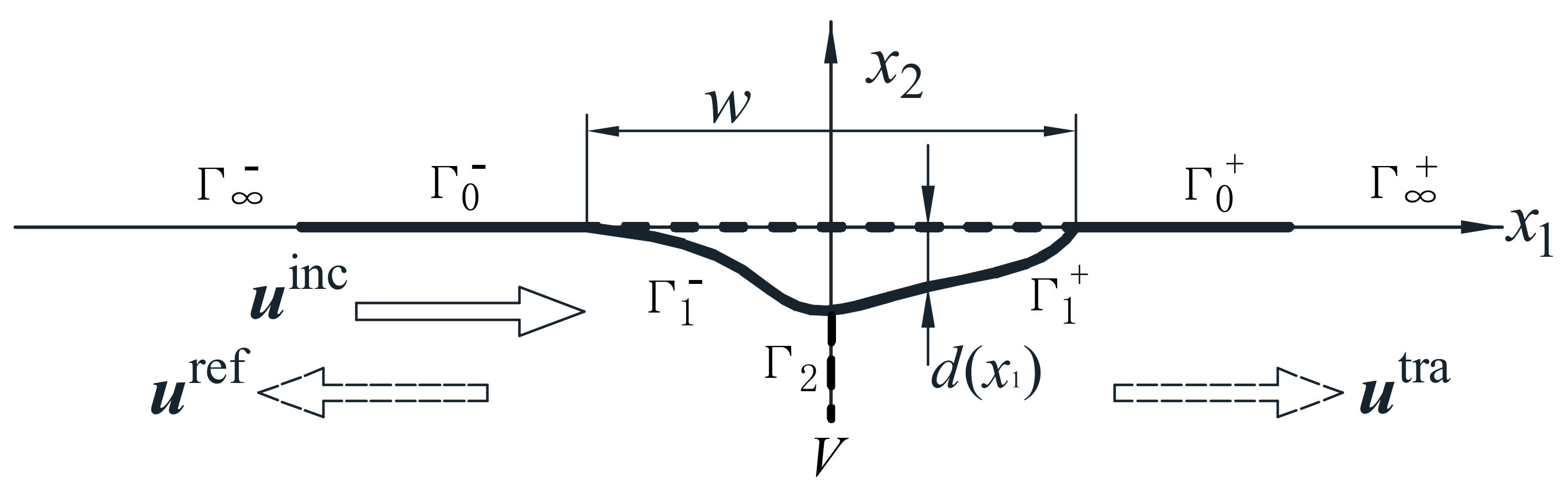
The problem to be solved is shown in Figure 1. An artificial canyon-shaped flaw has been cut on the surface of an isotropic elastic half-space. The incident Rayleigh wave propagates from left to the right side, and the reflected wave is observed at the far end of the left side.

For accurately computing the scattering wave field, we divide the forward analysis into two major steps, as shown in Figure 2.

(i) A time-harmonic incident Rayleigh wave field in the intact half-space is considered, and the correspondent stress ${\sigma }_{ij}^{\mathrm{inc}}$ is calculated along the curve ${\mathsf{\Gamma }}_1^{-}$, which is actually the flaw surface.

(ii)Since the actual traction on ${\mathsf{\Gamma }}_1^{-}$ is zero, the stress ${\sigma }_{ij}^{\mathrm{inc}}$ is released by exerting a compensation traction $t_i^{\mathrm{sca}}=-{\sigma }_{ij}^{\mathrm{inc}}{n}_j$ along ${\mathsf{\Gamma }}_1^{-}$. The scattering problem is transformed into the question of solving the wave field in the flawed half-space subjected to load $t_i^{\mathrm{sca}}$.

Then, the displacement in frequency domain of scattering wave field at an arbitrary point can be expressed in the form of boundary integral equation (BIE), as shown by Equation (1) [34].

$$c_{pi}\left(X\right)u_i^{\mathrm{sca}}\left(X,\omega \right)={\int }_{\mathsf{\Gamma }}\left[G_{ip}\left(x,X,\omega \right)t_i^{\mathrm{sca}}\left(x,\omega \right)-T_{ip}\left(x,X,\omega \right)u_i^{\mathrm{sca}}\left(x,\omega \right)\right]d\mathsf{\Gamma }(x)(i,p=1,2)$$

(1)

where $u_i^{\mathrm{sca}}$ and $t_i^{\mathrm{sca}}$ are displacement and boundary traction, respectively. $G_{ip}\left(x,X,\omega \right)$ and $T_{ip}\left(x,X,\omega \right)$ are fundamental solutions representing the i-th component of the displacement and stress at point x due to a unit time-harmonic concentrated load of angular frequency $\omega$ exerted in the p-th direction at point X in the elastic full-space. The coefficient $c_{pi}\left(X\right)={\delta }_{pi}$ for $X\in V$, $c_{pi}\left(X\right)={\delta }_{pi}/2$ for point $X\in \mathsf{\Gamma }$ which is smooth locally, $c_{pi}\left(X\right)=0$ for $X\notin V\cup \mathsf{\Gamma }$. It should be noted that here the boundary $\mathsf{\Gamma }$ includes both the flaw area and the intact infinite surface, as the full-space fundamental solutions have been chosen.

Now the whole surface is divided into six parts, ${\mathsf{\Gamma }}_{\infty }^{-}$ and ${\mathsf{\Gamma }}_{\infty }^{+}$ tending to infinity on the left and right side, respectively; ${\mathsf{\Gamma }}_0^{-}$ and ${\mathsf{\Gamma }}_0^{+}$ representing the near-field boundaries; ${\mathsf{\Gamma }}_1^{-}$ and ${\mathsf{\Gamma }}_1^{+}$ the left and right half of the flaw surface, respectively. Consequently, the scattered wave field is rewritten from Equation (1):

$$c_{pi}\left(X\right)u_i^{\mathrm{sca}}\left(X,\omega \right)=-{{\displaystyle \int }}_{{\mathsf{\Gamma }}_{\infty }^{-}\cup {\mathsf{\Gamma }}_{\infty }^{+}}{T}_{ip}\left(x,X,\omega \right)u_i^{\mathrm{sca}}\left(x,\omega \right)d\mathsf{\Gamma }(x)-{{\displaystyle \int }}_{{\mathsf{\Gamma }}_0^{-}\cup {\mathsf{\Gamma }}_0^{+}}{T}_{ip}\left(x,X,\omega \right)u_i^{\mathrm{sca}}\left(x,\omega \right)d\mathsf{\Gamma }(x)+{{\displaystyle \int }}_{{\mathsf{\Gamma }}_1^{-}\cup {\mathsf{\Gamma }}_1^{+}}[G_{ip}\left(x,X,\omega \right)t_i^{\mathrm{sca}}(x,\omega )-T_{ip}\left(x,X,\omega \right)u_i^{\mathrm{sca}}\left(x,\omega \right)]d\mathsf{\Gamma }(x), (i,p=1,2)$$

(2)

where the traction-free boundary condition on ${\mathsf{\Gamma }}_0^{-}\cup {\mathsf{\Gamma }}_0^{+}\cup {\mathsf{\Gamma }}_{\infty }^{-}\cup {\mathsf{\Gamma }}_{\infty }^{+}$ has been taken into account.

For traditional BEM, only the near-field boundaries ${\mathsf{\Gamma }}_0^{-}\cup {\mathsf{\Gamma }}_0^{+}\cup {\mathsf{\Gamma }}_1^{-}\cup {\mathsf{\Gamma }}_1^{+}$ are meshed, thus, the first item on the right hand side of Equation (2) is omitted. This treatment can cause spurious reflected waves at the truncation points which do not attenuate in the 2D half-space, which are unwanted.

It is noticed that, if the truncation point is far enough from the flaw area, the displacement fields on the infinite boundaries will follow a Rayleigh wave pattern travelling out of the flaw region [18], as expressed by

$$\begin{array}{c}{u}_i^{\mathrm{sca}}\left(x,\omega \right)\approx R^{-}\left(\omega \right){\tilde{u}}_i^{-}\left(x,\omega \right), x\in {\mathsf{\Gamma }}_{\infty }^{-}\\ u_i^{\mathrm{sca}}\left(x,\omega \right)\approx R^{+}\left(\omega \right){\tilde{u}}_i^{+}\left(x,\omega \right), x\in {\mathsf{\Gamma }}_{\infty }^{+}\end{array}$$

(3)

where ${\tilde{u}}_i^{\pm }$. is the displacement field of the unitary Rayleigh wave travelling in positive (+) or negative (−) directions, and $R^{\pm }$ the coefficient to be solved. Equation (3) makes it possible to take the far-field integrals in Equation (2) into consideration. Then, for any point on the boundary which is locally smooth, we have

$$\frac{1}{2}{u}_p^{\mathrm{sca}}\left(X,\omega \right)+R^{-}\left(\omega \right)A_p^{-}\left(X,\omega \right)+R^{+}\left(\omega \right)A_p^{+}\left(X,\omega \right)+{{\displaystyle \int }}_{{\mathsf{\Gamma }}_0^{-}{{\displaystyle \cup }}^{\text{}}{\mathsf{\Gamma }}_0^{+}{{\displaystyle \cup }}^{\text{}}{\mathsf{\Gamma }}_1^{-}{{\displaystyle \cup }}^{\text{}}{\mathsf{\Gamma }}_1^{+}}{T}_{ip}\left(x,X,\omega \right)u_i^{\mathrm{sca}}\left(x,\omega \right)d\mathsf{\Gamma }\left(x\right)={{\displaystyle \int }}_{{\mathsf{\Gamma }}_0^{-}{{\displaystyle \cup }}^{\text{}}{\mathsf{\Gamma }}_0^{+}}{G}_{ip}\left(x,X,\omega \right)t_i^{\mathrm{sca}}\left(x,\omega \right)d\mathsf{\Gamma }\left(x\right), \left(i,p=1,2\right).$$

(4)

where the correction terms $A_p^{\pm }$ having the definition $A_p^{-}\left(X,\omega \right)={{\displaystyle \int }}_{{\Gamma }_{\infty }^{-}}{T}_{ip}\left(x,X,\omega \right){\tilde{u}}_i^{-}\left(x,\omega \right)d\mathsf{\Gamma }\left(x\right)$ and $A_p^{+}\left(X,\omega \right)={{\displaystyle \int }}_{{\mathsf{\Gamma }}_{\infty }^{+}}{T}_{ip}\left(x,X,\omega \right){\tilde{u}}_i^{+}\left(x,\omega \right)d\mathsf{\Gamma }\left(x\right)$. They are constants. In paper [18], the coefficients $R^{\pm }$ are not explicit in the modified BEM formulation, consequently, the reflection coefficients obtained from x₁ and x₂ components of displacement might not coincide with each other. As an improvement, we will try to solve $R^{\pm }$ together with displacement fields.

The correction terms $A_p^{\pm }$ involve the integral over an infinite boundary, however, by applying the reciprocity theorem, the integral can be transferred to a bounded region [18,35].

$$A_p^{+}\left(X,\omega \right)=c_{pi}\left(X\right){\tilde{u}}_i^{+}\left(X,\omega \right)-\underset{{\mathsf{\Gamma }}_0^{+}}{\overset{}{{\displaystyle \int }}}{T}_{ip}\left(x,X,\omega \right){\tilde{u}}_i^{+}\left(x,\omega \right)d\mathsf{\Gamma }\left(x\right)+{{\displaystyle \int }}_{{\mathsf{\Gamma }}_1^{+}{{\displaystyle \cup }}^{\text{}}{\mathsf{\Gamma }}_2}[G_{ip}\left(x,X,\omega \right){\tilde{t}}_i^{+}\left(x,\omega \right)-T_{ip}\left(x,X,\omega \right){\tilde{u}}_i^{+}\left(x,\omega \right)]d\mathsf{\Gamma }\left(x\right)\hspace{1em}\left(i,p=1,2\right)$$

(5)

$$A_p^{-}\left(X,\omega \right)=c_{pi}\left(X\right){\tilde{u}}_i^{-}\left(X,\omega \right)-{{\displaystyle \int }}_{{\mathsf{\Gamma }}_0^{+}}{T}_{ip}\left(x,X,\omega \right){\tilde{u}}_i^{-}\left(x,\omega \right)d\mathsf{\Gamma }\left(x\right)+\underset{{\mathsf{\Gamma }}_1^{+}{{\displaystyle \cup }}^{\text{}}{\mathsf{\Gamma }}_2}{\overset{}{{\displaystyle \int }}}\left[G_{ip}\left(x,X,\omega \right){\tilde{t}}_i^{-}\left(x,\omega \right)-T_{ip}\left(x,X,\omega \right){\tilde{u}}_i^{-}\left(x,\omega \right)\right]d\mathsf{\Gamma }\left(x\right)\hspace{1em}\left(i,p=1,2\right)$$

(6)

where ${\mathsf{\Gamma }}_2$ represents an auxiliary vertical boundary of 2–3 Rayleigh wavelengths, see Figure 2. ${\tilde{t}}_i^{+}=-{\tilde{\sigma }}_{i1}^{+}{n}_1$ , and ${\tilde{t}}_i^{-}={\tilde{\sigma }}_{i1}^{-}{n}_1$ are defined on ${\mathsf{\Gamma }}_2$ with $n_1$ the unit normal vector pointing in positive x1-direction. ${\tilde{\sigma }}_{i1}^{\pm }$ is the stress field of the unitary Rayleigh wave propagating in positive or negative x1-directions, respectively.

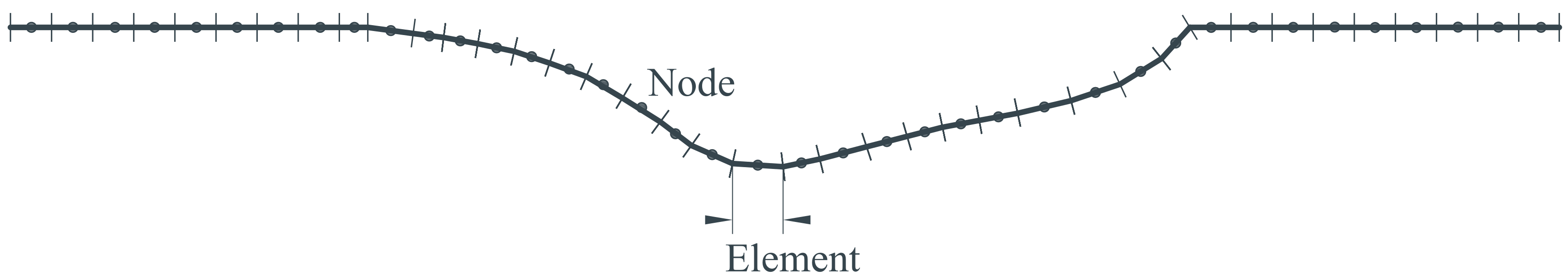
By substitution of Equations (5) and (6) into Equation (4), we can obtain an equation set with the displacement and coefficients $R^{\pm }$ as the undetermined variables. Here, we adopt the constant elements (see Figure 3) in the BEM discretization, in which one element is represented by the only node in the middle, and obtain the matrix representation in the form of

$$\left[T\right]\left\{{\mathrm{u}}^{\mathrm{sca}}\right\}=\left[G\right]\left\{{\mathrm{t}}^{\mathrm{sca}}\right\}$$

(7)

Here, we assume that for the 1st or the N-th node, the displacements are not independent, and can be expressed as $R^{-}\left(\omega \right){\tilde{u}}_i^{-}\left(x_1,\omega \right)$ and $R^{+}\left(\omega \right){\tilde{u}}_i^{+}\left(x_N,\omega \right)$, respectively, where $x_1$ and $x_N$ are coordinates of the 1st and the N-th node, respectively. Thus, the submatrices concerning the 1st and the N-th elements in $\left[T\right]$ are combined with the correction terms $A_p^{\pm }$, and placed as the first and last columns. Consequently, the vector $\left\{{\mathrm{u}}^{\mathrm{sca}}\right\}$ contains the displacements of nodes 2~(N − 1), together with coefficients $R^{\pm }$, as shown by

$$\left\{{\mathrm{u}}^{\mathrm{sca}}\right\}={\left[\begin{array}{cccccccccc}{R}^{-}& u_{21}& u_{22}& \dots & u_{P1}& u_{P2}& \dots & u_{\left(N-1\right)1}& u_{\left(N-1\right)2}& R^{+}\end{array}\right]}^T$$

(8)

where $u_{Pi}$ represents the displacement in ith direction at the Pth node.

The matrix $\left[T\right]$ is expressed in detail as

$$[T]=\left[\begin{array}{cccccccccc}{S}_{11}^{-}& T_{2111}& T_{2211}& \dots & T_{p111}& T_{p211}& \dots & T_{(N-1)111}& T_{(N-1)211}& S_{11}^{+}\\ S_{12}^{-}& T_{2112}& T_{2212}& \dots & T_{p112}& T_{p112}& \dots & T_{(N-1)112}& T_{(N-1)212}& S_{12}^{+}\\ ⋮& ⋮& ⋮& & ⋮& ⋮& & ⋮& ⋮& ⋮\\ S_{j1}^{-}& T_{21j1}& T_{22j1}& \dots & T_{p1j1}& T_{p2j1}& \dots & T_{(N-1)1j1}& T_{(N-1)2j1}& S_{j1}^{+}\\ S_{j2}^{-}& T_{21j2}& T_{22j2}& \dots & T_{p1j2}& T_{p1j2}& \dots & T_{(N-1)1j2}& T_{(N-1)2j2}& S_{j2}^{+}\\ ⋮& ⋮& ⋮& & ⋮& ⋮& & ⋮& ⋮& ⋮\\ S_{N1}^{-}& T_{21N1}& T_{21N1}& \dots & T_{p1N1}& T_{p2N1}& \dots & T_{(N-1)1N1}& T_{(N-1)2N1}& S_{N1}^{+}\\ S_{N2}^{-}& T_{21N1}& T_{21N1}& \dots & T_{p1N2}& T_{p1N2}& \dots & T_{(N-1)1N2}& T_{(N-1)2N2}& S_{N2}^{+}\end{array}\right]$$

(9)

The elements in the first and last columns are defined as

$$\begin{array}{c}{S}_{J1}^{-}=A_{J1}^{-}+T_{11J1}{\tilde{u}}_{11}^{-}+T_{12J1}{\tilde{u}}_{12}^{-},S_{J2}^{-}=A_{J2}^{-}+T_{11J2}{\tilde{u}}_{11}^{-}+T_{12J2}{\tilde{u}}_{12}^{-}\\ S_{J1}^{+}=T_{N1J1}{\tilde{u}}_{N1}^{+}+T_{N2J1}{\tilde{u}}_{N2}^{+}+A_{J1}^{+},S_{J2}^{+}=T_{N1J2}{\tilde{u}}_{N1}^{+}+T_{N2J2}{\tilde{u}}_{N2}^{+}+A_{J2}^{+}\end{array}$$

(10)

in which, $A_{Ji}^{\pm }=A_i^{\pm }\left(x_J\right)$, obtained from Equations (5) and (6), and the elements $T_{PiJk}=\left(1/2\right){\delta }_{Pj}{\delta }_{ik}+{\int }_{{\mathsf{\Gamma }}_P}{T}_{ik}\left(x,x_J,\omega \right)d\mathsf{\Gamma }$, (i, k = 1, 2). The size of matrix $\left[T\right]$ is 2N × 2(N − 1), and $\left\{u^{sca}\right\}$ 2(N − 1) × 1.

On the other hand, $\left[G\right]$ is a 2N × 2N₀ sized matrix, $\left\{t^{sca}\right\}$ is a 2N₀ × 1 sized vector, where N₀ is the number of nodes on which the tractions are nonzero. The elements in $\left[G\right]$ can be written as $G_{PiJk}={\int }_{{\mathsf{\Gamma }}_P}{T}_{ik}\left(x,x_J,\omega \right)d\mathsf{\Gamma }$, and the elements in $\left\{t^{sca}\right\}$ is $t_{Pi}^{\mathrm{sca}}\left(x,x_J,\omega \right)$.

Since the matrix $\left[T\right]$ is not square-sized, the equation is solved in the least-square sense to achieve error minimization. In the final solution, we can obtain reflection coefficient $R^{-}$ at the first and transmission coefficient $R^{+}$. at the last element simultaneously, as well as the whole near-field displacements.

2.2. Verification of Reflection Coefficients

For verification of the reflection coefficients obtained from Equation (7), we adopt the scattering equation in half-space, which uses the half-space Green’s function to calculate the far-field wave pattern, as shown in [36]:

$$u_n^{\mathrm{sca}}\left(X\right)={{\displaystyle \int }}_{{\mathsf{\Gamma }}_1^{-}{{\displaystyle \cup }}^{\text{}}{\mathsf{\Gamma }}_1^{+}}{C}_{ijkl}{n}_j\left(x\right)\frac{\partial G_{ln}^{\mathrm{H}}\left(x,X\right)}{\partial x_k}{u}_n^{\mathrm{inc}}\left(x\right)d\mathsf{\Gamma }\left(x\right) \left(i,j,k,l=1, 2\right)$$

(11)

where $C_{ijkl}$ is the stiffness tensor, $n_j$ is the unit normal vector pointing outward the flaw area, and $G_{ln}^{\mathrm{H}}\left(x,X\right)$ represents the Green’s functions in the half-space. In the far-field, the half-space Green’s function can be expressed in the Rayleigh wave form [37]:

$$G_{\alpha \beta }^{\mathrm{H}}\left(x,X\right)=f\left({\xi }_0\right)A{p}_{\alpha }\left(x_2\right)B{p}_{\beta }\left(X_2\right)e^{+i{\xi }_0\left(x_1-X_1\right)},\left(\alpha , \beta =1, 2\right).$$

(12)

where

$$\begin{array}{c}A=\{\begin{array}{c}-1 \left(i=2, x_1<X_1\right)\\ 1 \mathrm{otherwise} \end{array}\dots B=\{\begin{array}{c}-1 \left(j=2, X_1<x_1\right)\\ 1 \mathrm{otherwise} \end{array}\\ p_1\left(x_2\right)=\frac{R_{\mathrm{T}0}}{{\xi }_0}{e}^{+R_{\mathrm{T}0}{x}_2}-\frac{{\xi }_0^2+R_{\mathrm{T}0}^2}{2R_{\mathrm{L}0}{\xi }_0}{e}^{+R_{\mathrm{L}0}{x}_2}\\ p_2\left(x_2\right)=-i{e}^{+R_{\mathrm{T}0}{x}_2}+i\frac{{\xi }_0^2+R_{\mathrm{T}0}^2}{2{\xi }_0^2}{e}^{+R_{\mathrm{L}0}{x}_2}\\ f\left({\xi }_0\right)=\frac{4i{\xi }_0^4{R}_{\mathrm{L}0}}{\mu k_{\mathrm{T}}^{2}F\prime \left({\xi }_0\right)}\\ F\left(\xi \right)={\left({\xi }^2+R_{\mathrm{T}0}^2\right)}^2-4{\xi }^2{R}_{\mathrm{L}0}{R}_{\mathrm{T}0}\end{array}$$

(13)

in which $k_{\mathrm{L}}=\omega /c_{\mathrm{L}}$, $k_{\mathrm{T}}=\omega /c_{\mathrm{T}}$, ${\xi }_0$ are wavenumbers of S, P, and Rayleigh waves, respectively, and $R_{\mathrm{L}0}^2={\xi }_0^2-k_{\mathrm{L}}^2$, $R_{\mathrm{T}0}^2={\xi }_0^2-k_{\mathrm{T}}^2$. The Rayleigh wavenumber ${\xi }_0$ satisfies $F\left({\xi }_0\right)=0$, and $F\prime \left({\xi }_0\right)$ is the derivative of $F\left(\xi \right)$ at $\xi ={\xi }_0$.

The reflection coefficients derived from Equation (11) should coincide with that obtained directly from Equation (7). A numerical example will be given to show the validity of reflection coefficients. Moreover, the scattering Equation (11) is more useful in the inverse reconstruction procedure of the flaw shape.

2.3. Results of Forward Problem

Example 1.

To verify the modified BEM method, we now try to solve the classical Rayleigh wave scattering problem presented by Kawase [10], for which the solutions have already been obtained from discrete wavenumber method applying half-space Green functions.

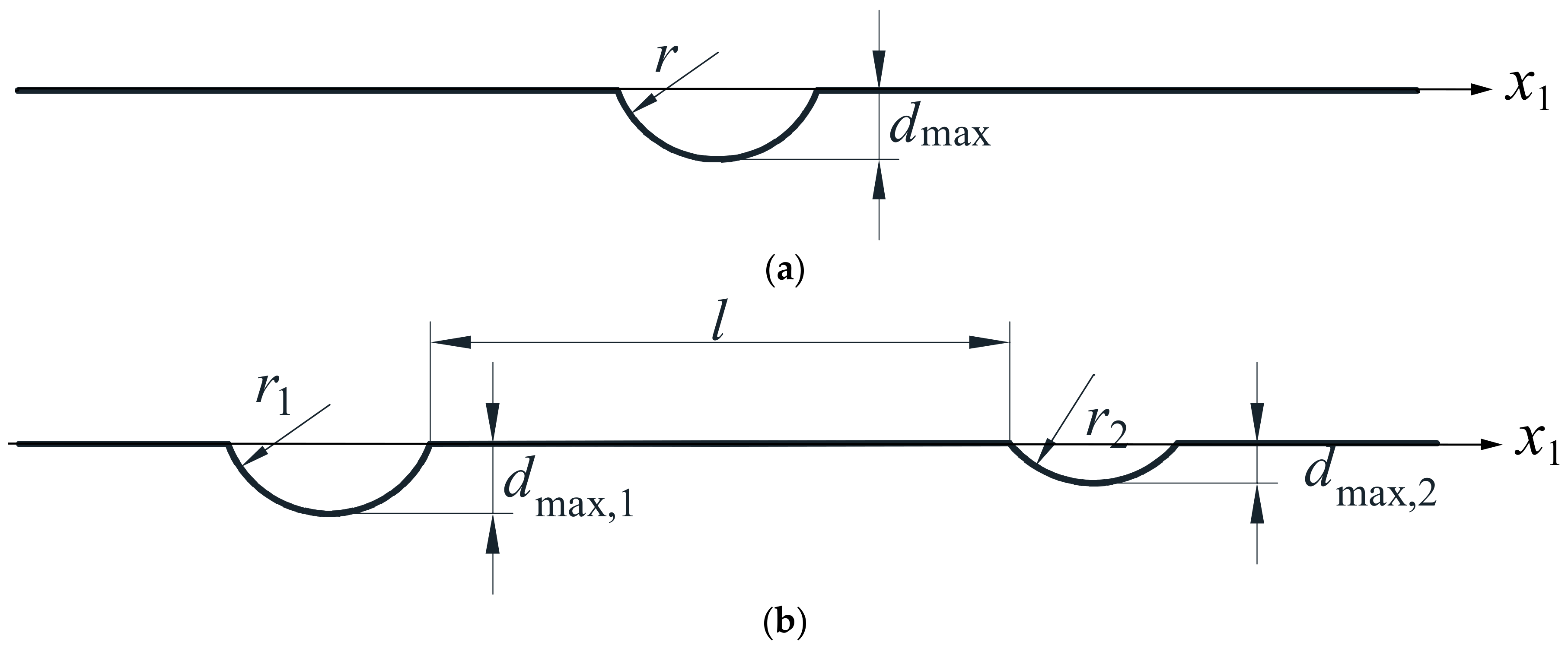
As shown by Figure 4a, an artificial half-circular canyon-shaped flaw is set on the surface of an isotropic elastic half-space, with Poisson’s ratio of 1/3. The incident wave is a unitary Rayleigh wave travelling from left to right, whose time-domain waveform is expressed as

$$u\left(T\right)=\left[1/2{\Omega }^2{\left(T-T_0\right)}^2-1\right]\exp \left[-{\left(\Omega /2\right)}^2{\left(T-T_0\right)}^2\right]$$

(14)

in which $\Omega =\omega r/c_{\mathrm{T}}$ is the normalized circular frequency, where r is the radius of canyon, and $c_{\mathrm{T}}$ is the shear wave velocity. $T=t{c}_{\mathrm{T}}/r$ represents the normalized time array. The time-domain signal is shown in Figure 5, when $\Omega =2\mathsf{\pi }$ and $T_0=2\mathsf{\pi }$.

We perform a Fourier transform to the incident wave signal in time-domain to obtain its frequency spectrum, and calculate the displacement field and reflection coefficients at each frequency point by the modified BEM. As an example, the whole displacement field along the surface at frequency $\Omega =2\mathsf{\pi }$ is plotted in Figure 6, and is compared with the results obtained by Kawase [10]. It is seen that the BEM displacements show good agreement with the previous results.

Displacement fields at other frequency points have also been calculated in the same manner. An inverse Fourier transform is then applied to the frequency-domain displacements to attain time-domain wave signals for different points along the surface, as shown in Figure 7a,b, from which we can see that the spurious reflection waves are not generated.

Example 2.

Similarly with Example 1, an artificial arc-shaped canyon is located on the surface of an isotropic elastic half-space, whose depth–radius ratio$d_{max}/r=0.2$ . The Poisson’s ratio is 1/3. We calculated the reflection coefficients in frequency domain within range $\Omega =\omega r/c_T$ from 0.2 to 5.0 at an interval of 0.2.

The circular dots in Figure 8 shows the reflection coefficients obtained directly from the modified BEM program, and the rectangular dots represents those derived from half-space scattering Equation (11). The good agreement illustrates the validity of the forward analysis.

This example will be used in the following inverse reconstruction.

3. Inverse Problem by Modified BEM

3.1. Formulation of Inverse Reconstruction

We now try to reconstruct the position and geometric properties of the canyon-shaped flaw. In order to quantitatively depict the flaw’s geometric characteristics, an objective function $d\left(x_1\right)$ is defined in $x_1$ domain, which means the flaw depth at coordinate $x_1$, whereas in the intact area, its value is zero.

The scattering Equation (11) in half-space is adopted for inversion. In this paper, a shallow flaw is considered, which can be thought of as a weak scatterer. In this case, the Born approximation [36] can be used for linearization, which replaces the total wave field by the incident wave field on flaw boundaries. e.g., $u_1^{\mathrm{tot}}\approx u_1^{\mathrm{inc}}$. Then Equation (11) becomes

$$u_n^{\mathrm{sca}}\left(X\right)\approx {{\displaystyle \int }}_{{\mathsf{\Gamma }}_1^{-}{{\displaystyle \cup }}^{\text{}}{\mathsf{\Gamma }}_1^{+}}{C}_{ijkl}{n}_j\left(x\right)\frac{\partial G_{ln}^{\mathrm{H}}\left(x,X\right)}{\partial x_k}{u}_n^{\mathrm{inc}}\left(x\right)d\mathsf{\Gamma }\left(x\right) \left(i,j,k,l,n=1, 2\right)$$

(15)

It is noticed that, on the original half-space surface ${\mathsf{\Gamma }}_1^{\prime }$ (see the dotted line in Figure 1), the traction induced by half-space Green functions is zero. Thus, the surface for integration can be extended to ${\mathsf{\Gamma }}_1^{-}{{\displaystyle \cup }}^{\text{}}{\mathsf{\Gamma }}_1^{+}{{\displaystyle \cup }}^{\text{}}{\mathsf{\Gamma }}_1^{\prime }$. Furthermore, after substitution of Lamé constant $\lambda$ and shear modulus $\mu$, the scattering equation is expanded as

$$\begin{array}{c}{u}_n^{\mathrm{sca}}\left(X\right)\approx {{\displaystyle \int }}_{{\mathsf{\Gamma }}_1^{-}{{\displaystyle \cup }}^{\text{}}{\mathsf{\Gamma }}_1^{+}{{\displaystyle \cup }}^{\text{}}{\mathsf{\Gamma }}_1^{\prime }}[\left(n_1\frac{\partial G_{1n}^{\mathrm{H}}}{\partial x_1}{u}_1^{\mathrm{inc}}+n_2\frac{\partial G_{1n}^{\mathrm{H}}}{\partial x_2}{u}_2^{\mathrm{inc}}\right)\left(\lambda +2\mu \right)+\left(n_2\frac{\partial G_{1n}^{\mathrm{H}}}{\partial x_1}{u}_2^{\mathrm{inc}}+n_1\frac{\partial G_{2n}^{\mathrm{H}}}{\partial x_1}{u}_1^{\mathrm{inc}}\right)\lambda \\ +\left(n_2\frac{\partial G_{2n}^{\mathrm{H}}}{\partial x_1}{u}_1^{\mathrm{inc}}+n_1\frac{\partial G_{1n}^{\mathrm{H}}}{\partial x_2}{u}_2^{\mathrm{inc}}+n_2\frac{\partial G_{1n}^{\mathrm{H}}}{\partial x_2}{u}_1^{\mathrm{inc}}+n_1\frac{\partial G_{2n}^{\mathrm{H}}}{\partial x_1}{u}_2^{\mathrm{inc}}\right)\mu ]d\mathsf{\Gamma }\left(x\right) (i,j,k,l,n=1,2)\end{array}$$

(16)

Since surface ${\mathsf{\Gamma }}_1^{-}{{\displaystyle \cup }}^{\text{}}{\mathsf{\Gamma }}_1^{+}{{\displaystyle \cup }}^{\text{}}{\mathsf{\Gamma }}_1^{\prime }$ is closed, we can perform Gauss’s theorem to the flawed region and obtain

$$\begin{array}{c}{u}_n^{\mathrm{sca}}\left(X\right)\approx {{\displaystyle \int }}_{\mathrm{V}}[\left(\frac{{\partial }^2{G}_{1n}^{\mathrm{H}}}{\partial x_1^2}{u}_1^{\mathrm{inc}}+\frac{\partial G_{1n}^{\mathrm{H}}}{\partial x_1}\frac{\partial u_1^{\mathrm{inc}}}{\partial x_1}+\frac{{\partial }^2{G}_{2n}^{\mathrm{H}}}{\partial x_2^2}{u}_2^{\mathrm{inc}}+\frac{\partial G_{2n}^{\mathrm{H}}}{\partial x_2}\frac{\partial u_2^{\mathrm{inc}}}{\partial x_2}\right)\left(\lambda +2\mu \right)\\ +\left(\frac{{\partial }^2{G}_{1n}^{\mathrm{H}}}{\partial x_1\partial x_2}{u}_2^{\mathrm{inc}}+\frac{\partial G_{1n}^{\mathrm{H}}}{\partial x_1}\frac{\partial u_2^{\mathrm{inc}}}{\partial x_2}+\frac{{\partial }^2{G}_{2n}^{\mathrm{H}}}{\partial x_1\partial x_2}{u}_1^{\mathrm{inc}}+\frac{\partial G_{2n}^{\mathrm{H}}}{\partial x_2}\frac{\partial u_1^{\mathrm{inc}}}{\partial x_1}\right)\lambda \\ +(\frac{{\partial }^2{G}_{2n}^{\mathrm{H}}}{\partial x_1\partial x_2}{u}_1^{\mathrm{inc}}+\frac{\partial G_{2n}^{\mathrm{H}}}{\partial x_1}\frac{\partial u_1^{\mathrm{inc}}}{\partial x_2}+\frac{{\partial }^2{G}_{1n}^{\mathrm{H}}}{\partial x_1\partial x_2}{u}_2^{\mathrm{inc}}+\frac{\partial G_{1n}^{\mathrm{H}}}{\partial x_2}\frac{\partial u_2^{\mathrm{inc}}}{\partial x_1}\\ +\frac{{\partial }^2{G}_{1n}^{\mathrm{H}}}{\partial x_2^2}{u}_1^{\mathrm{inc}}+\frac{\partial G_{1n}^{\mathrm{H}}}{\partial x_2}\frac{\partial u_1^{\mathrm{inc}}}{\partial x_2}+\frac{{\partial }^2{G}_{2n}^{\mathrm{H}}}{\partial x_1^2}{u}_2^{\mathrm{inc}}+\frac{\partial G_{2n}^{\mathrm{H}}}{\partial x_1}\frac{\partial u_2^{\mathrm{inc}}}{\partial x_1})\mu ]d\mathsf{\Gamma }\left(x\right) (i,j,k,l,n=1,2)\end{array}$$

(17)

It is assumed that a pure incident Rayleigh wave mode is sent from left to right, and the reflected wave is observed at the far field on the left side. Thus, the incident wave with wavenumber ${\xi }_0$ can be expressed as

$$\begin{array}{c}{u}_1^{\mathrm{inc}}\left(x,{\xi }_0\right)=A^{\mathrm{inc}}\left({\xi }_0\right)p_1\left(x_2\right)e^{+i{\xi }_0{x}_1}\\ u_2^{\mathrm{inc}}\left(x,{\xi }_0\right)=A^{\mathrm{inc}}\left({\xi }_0\right)p_2\left(x_2\right)e^{+i{\xi }_0{x}_1}\end{array}$$

(18)

where $p_i\left(x_2\right)$ (i = 1, 2) is defined in Equation (13), and $A^{\mathrm{inc}}$ represents the complex amplitude of the incident wave.

We use the far-field form of half-space Green’s functions (12), and substitute them into Equation (17), and obtain the reflected wave of the same wave number ${\xi }_0$, as shown by Equation (19):

$$\begin{array}{c}{u}_n^{\mathrm{sca}}\left(X,{\xi }_0\right)\approx A^{\mathrm{inc}}\left({\xi }_0\right){{\displaystyle \int }}_{\mathrm{V}}[\left(-2{\xi }_0^2{p}_1^2\left(x_2\right)+\frac{d^2{p}_2\left(x_2\right)}{d{x}_2^2}{p}_2\left(x_2\right)+{\left(\frac{d{p}_2\left(x_2\right)}{d{x}_2}\right)}^2\right)\left(\lambda +2\mu \right)\\ +\left(i{\xi }_0\frac{d{p}_1\left(x_2\right)}{d{x}_2}{p}_2\left(x_2\right)\right)\left(\lambda +3\mu \right)+\left(i{\xi }_0\frac{d{p}_2\left(x_2\right)}{d{x}_2}{p}_1\left(x_2\right)\right)\left(3\lambda +\mu \right)\\ +\left(-2{\xi }_0^2{p}_2^2\left(x_2\right)+\frac{d^2{p}_1\left(x_2\right)}{d{x}_2^2}{p}_1\left(x_2\right)+{\left(\frac{d{p}_1\left(x_2\right)}{d{x}_2}\right)}^2\right)\mu ]·e^{+i{\xi }_0·2x_1}dV·f({\xi }_0) ·p_n\left(X_2\right)e^{-i{\xi }_0·X_1}\\ \left(i,j,k,l,n=1,2\right)\end{array}$$

(19)

If one takes a thorough observation on Equation (19), he can find that $p_n\left(X_2\right)\exp \left(-i{\xi }_0·X_1\right)$ represents a unitary reflected Rayleigh wave travelling from right to left, and the integral over V is taken with respect to coordinate x of field points, and can be viewed as a complex amplitude of that unitary reflected Rayleigh wave. Also, the integrand is separated into the part in the bracket concerning $x_2$ coordinate, and an exponential item $\exp \left(+i{\xi }_0·2x_1\right)$.

This inspires us to rewrite the expression of reflected wave into the following form

$$\begin{array}{c}{u}_n^{\mathrm{sca}}\left(X,{\xi }_0\right)\approx A^{\mathrm{inc}}\left({\xi }_0\right)f\left({\xi }_0\right)·{{\displaystyle \int }}_{\mathrm{V}}\mathrm{Fun}\left(x_2, {\xi }_0\right)\exp \left(+i{\xi }_0·2x_1\right)dV·p_n\left(X_2\right)\exp \left(-i{\xi }_0·X_1\right)\\ \equiv A^{\mathrm{ref}}\left({\xi }_0\right)p_n\left(X_2\right)\exp \left(-i{\xi }_0·X_1\right)\end{array}$$

(20)

where the $\mathrm{Fun}\left(x_2,{\xi }_0\right)$ is the expression in the bracket in Equation (19), and the complex amplitude for the reflected wave is termed as $A^{\mathrm{ref}}$. Now we define the reflection coefficient $C^{\mathrm{ref}}\left({\xi }_0\right)$ as the ratio between $A^{\mathrm{ref}}\left({\xi }_0\right)$ and $A^{\mathrm{inc}}\left({\xi }_0\right)$, so that

$$C^{\mathrm{ref}}\left({\xi }_0\right)\approx f\left({\xi }_0\right)·{{\displaystyle \int }}_{\mathrm{V}}\mathrm{Fun}\left(x_2, {\xi }_0\right)\exp \left(+i{\xi }_0·2x_1\right)dV$$

(21)

Also, the volume integral is further rewritten as a dual integral:

$${{\displaystyle \int }}_{\mathrm{V}}\mathrm{Fun}\left(x_2, {\xi }_0\right)\exp \left(+i{\xi }_0·2x_1\right)dV={{\displaystyle \int }}_{-\infty }^{\infty }\exp \left(+i{\xi }_0·2x_1\right)d{x}_1{{\displaystyle \int }}_{-d\left(x_1\right)}^0\mathrm{Fun}\left(x_2, {\xi }_0\right)d{x}_2$$

(22)

where $d\left(x_1\right)$ is the flaw depth at coordinate $x_1$. The integral range has been extended from minus infinity to infinity, since $d\left(x_1\right)=0$ in the intact areas.

After organization, the reflection coefficient is expressed as

$$\begin{array}{c}{C}^{\mathrm{ref}}\left({\xi }_0\right)\approx {{\displaystyle \int }}_{-\infty }^{\infty }{e}^{+i{\xi }_0·2x_1}d{x}_1{{\displaystyle \int }}_{-d\left(x_1\right)}^0\left(c_{\mathrm{TT}}\left({\xi }_0\right)e^{+2R_{\mathrm{T}0}{x}_2}+c_{\mathrm{TL}}\left({\xi }_0\right)e^{+2\left(R_{\mathrm{T}0}+R_{\mathrm{L}0}\right)x_2}+c_{\mathrm{LL}}\left({\xi }_0\right)e^{+2R_{\mathrm{L}0}{x}_2}\right)d{x}_2\end{array}$$

(23)

where $c_{\mathrm{TT}}$, $c_{\mathrm{TL}}$, and $c_{\mathrm{LL}}$ are functions of wavenumber ${\xi }_0$, and are expressed in detail as

$$\begin{array}{c}{c}_{\mathrm{TT}}\left({\xi }_0\right)=2\mu \frac{k_{\mathrm{T}0}^4}{{\xi }_0^2}\\ c_{\mathrm{TL}}\left({\xi }_0\right)=\frac{{\xi }_0^2+R_{\mathrm{T}0}^2}{2{\xi }_0^2{R}_{\mathrm{L}0}}\left(\lambda k_{\mathrm{L}0}^2\left(R_{\mathrm{T}0}-R_{\mathrm{L}0}\right)+\mu \left(7{\xi }_0^2{R}_{\mathrm{T}0}-5{\xi }_0^2{R}_{\mathrm{L}0}+4R_{\mathrm{L}0}^3-R_{\mathrm{T}0}^3-R_{\mathrm{L}0}{R}_{\mathrm{T}0}^2+6R_{\mathrm{L}0}^2{R}_{\mathrm{T}0}\right)\right)\\ c_{\mathrm{LL}}\left({\xi }_0\right)=-\left(\lambda +2\mu \right)\frac{k_{\mathrm{L}0}^4{\left({\xi }_0^2+R_{\mathrm{T}0}^2\right)}^2}{2{\xi }_0^4{R}_{\mathrm{L}0}^2}\end{array}$$

(24)

If we perform an integral over $x_2$ first, we can rewrite Equation (23) as

$$C^{\mathrm{ref}}\left({\xi }_0\right)\approx {{\displaystyle \int }}_{-\infty }^{\infty }\left[c_{\mathrm{TT}}\left({\xi }_0\right)\frac{1-e^{-2R_{\mathrm{T}0}d\left(x_1\right)}}{2R_{\mathrm{T}0}}+c_{\mathrm{TL}}\left({\xi }_0\right)\frac{1-e^{-\left(R_{\mathrm{T}0}+R_{\mathrm{L}0}\right)d\left(x_1\right)}}{R_{\mathrm{T}0}+R_{\mathrm{L}0}}+c_{\mathrm{LL}}\left({\xi }_0\right)\frac{1-e^{-2R_{\mathrm{L}0}d\left(x_1\right)}}{2R_{\mathrm{L}0}}\right]e^{+i{\xi }_0·2x_1}d{x}_1$$

(25)

Since the flaw depth is considered small, it is natural to apply Taylor expansion for the exponential functions in Equation (25) at $d\left(x_1\right)=0$, i.e.,

$$C^{\mathrm{ref}}\left({\xi }_0\right)\approx {{\displaystyle \int }}_{-\infty }^{\infty }\left[c_{\mathrm{TT}}\left({\xi }_0\right)+c_{\mathrm{TL}}\left({\xi }_0\right)+c_{\mathrm{LL}}\left({\xi }_0\right)\right]d\left(x_1\right)e^{+i{\xi }_0·2x_1}d{x}_1$$

(26)

Then, it is found that the objective function $d\left(x_1\right)$ can be reconstructed using a spatial inverse Fourier transform, as illustrated by

$$d\left(x_1\right)\approx \frac{1}{2\mathsf{\pi }}{{\displaystyle \int }}_{-\infty }^{\infty }\frac{C^{\mathrm{ref}}\left({\xi }_0\right)}{c_{\mathrm{TT}}\left({\xi }_0\right)+c_{\mathrm{TL}}\left({\xi }_0\right)+c_{\mathrm{LL}}\left({\xi }_0\right)}{e}^{-i{x}_1·2{\xi }_0}d\left(2{\xi }_0\right)$$

(27)

It should be noted that the inversion formula adopts a series of assumptions for linearization. Thus, parametric analysis should be performed to show the validity range of this method.

3.2. Numerical Examples

In this sub-section, numerical examples are given to show the validity of the inversion procedure. Also, parametric studies are performed to illustrate which kind of flaw is the most suitable for this reconstruction method.

Here, we mainly focus on the arc-shaped canyons as representatives of surface flaws. It is believed that other shapes can lead to similar conclusions.

3.2.1. Choice of Parameters

The radius $\mathrm{r}$, maximum depth $d_{\max }$ in Figure 4a, as well as the distance $\mathrm{l}$ in Figure Figure 4b for the double-flaw case, are the key geometric parameters for arc-shaped canyons; the maximum frequency ${\omega }_{\max }$ is an important parameter of input data.

For generality, we perform dimensionless analysis in this paper. The normalized radius $R=r/r$ is kept constant as 1; the depth is normalized as $D=d/r$; and frequency $\Omega =\omega r/c_{\mathrm{T}}$, where ${\mathrm{c}}_{\mathrm{T}}$ is the shear wave velocity in the half-space. Meanwhile, the normalized coordinates are written as $X_i=x_i/r$ (i = 1, 2.)

The readers can readily verify that, in dimensionless analysis, the model (i) with radius $r$, maximum depth $d_{\max }$, and frequency range $0~{\omega }_{\max }$, is equivalent to model (ii) with radius $2r$, maximum depth $2d_{\max }$, and frequency range $0~0.5{\omega }_{\max }$. Thus, the absolute value of radius is of little importance. Instead, the depth–radius ratio $d_{\max }/r$ (or $D_{\max }/R$) is a more essential parameter showing the “steepness” of the canyon. Another important factor is the normalized frequency range, which reflects the incident Rayleigh wavelength in comparison with the geometric flaw scale.

3.2.2. Reconstruction Results for Models of Different Depth–Radius Ratio

We established three canyon models with depth–radius ratios $d_{\max }/r$ equaling 0.1, 0.2, and 0.5, respectively. For each model, we calculated the reflection coefficients of Rayleigh wave within the frequency range from $0$ to ${\Omega }_{\max }=5.0$, with a uniform interval of $\mathrm{d}\Omega =0.2$, as can be illustrated in Figure 8. These coefficients are substituted into the inversion Equation (27) to obtain the flaw depth function $d\left(x_1\right)$.

It should be noted, Equation (27) takes an integral from minus to positive infinity. However, the reflection coefficients are only available at positive wavenumber points. Since $d\left(x_1\right)$ is a real function, we can define $C^{\mathrm{ref}}\left(-{\xi }_0\right)$ as the complex conjugate of $C^{\mathrm{ref}}\left({\xi }_0\right)$ (for ${\xi }_0>0$), i.e., $C^{\mathrm{ref}}\left(-{\xi }_0\right)=C^{\mathrm{ref}*}\left({\xi }_0\right)$. The functions $c_{\mathrm{TT}}\left({\xi }_0\right)$, $c_{\mathrm{TL}}\left({\xi }_0\right)$, and $c_{\mathrm{LL}}\left({\xi }_0\right)$ are also defined similarly. The whole integrand function is defined as 0 at ${\xi }_0=0$. Moreover, the integration range is reduced to $0~{\Omega }_{\max }$.

After discretization, the integral of Equation (27) becomes

$$d\left(p\Delta x_1\right)={\displaystyle \sum }_{k=0}^{N-1}\left(\frac{C^{\mathrm{ref},k}\exp \left(-2i\mathsf{\pi }pk/N\right)}{c_{\mathrm{TT}}^k+c_{\mathrm{TL}}^k+c_{\mathrm{LL}}^k}+\frac{C^{\mathrm{ref},k*}\exp \left(+2i\mathsf{\pi }pk/N\right)}{c_{\mathrm{TT}}^{k*}+c_{\mathrm{TL}}^{k*}+c_{\mathrm{LL}}^{k*}}\right)·2\Delta {\xi }_0$$

(28)

where $\Delta x_1=\mathsf{\pi }/N\Delta {\xi }_0$ is the increment in $x_1$ coordinate. Integers p and k are indices in spatial and wavenumber series, respectively. The discrete inverse Fourier transform is easily performed by FFT (Fast Fourier Transform) algorithm.

The results are plotted in Figure 9. It is observed that when ratio $d_{\max }/r$ is as small as 0.1 (see Figure 9a), the geometric properties (such as location, depth, and width) and shape of the flaw can be reconstructed with good precision. When $d_{\max }/r$ value increases to 0.5 (see Figure 9c), the location of flaw can still be precisely detected, and the width and depth are slightly larger than the reality. However, the reconstructed shape is not as accurate as its shallower counterparts. The image underestimates the bottom region, and looks as if there were two local maximum depth points. The reason why the shallow and flat flaws are reconstructed better can be attributed to the application range of Born approximation, which is especially suitable for weak scatterers.

Even the reconstructed image is not accurate for deeper and steeper canyons, the geometric characteristics (e.g., location, depth, and width) can be obtained with acceptable accuracy, so the image can be used as the “initial solution” in the following iterative reconstruction algorithm.

3.2.3. Reconstruction Results Using Different Frequency Range

It is necessary to discuss how the frequency range affects the inverse reconstruction results, which helps us understand the proper choice of incident wavelength in experiments. We have recalculated the inverse reconstruction for the flaws with $d_{\max }/r$ equaling 0.2 and 0.5, using frequency range $\Omega =0~5.0$, $0~2.0$, and $0~1.0$, respectively.

The reconstruction results are plotted in Figure 10. For the case of $d_{\max }/r=0.2$ (see Figure 10a), the frequency range of $\Omega =0~1.0$ (see the dash-dot curve) only gives a vague image, yet it still obtains the correct location. When the frequency range increases to $\Omega =0~2.0$, the flaw shape seems to agree well with the reality, however, the image underestimates the flaw depth and overestimates the width. As the full data of reflection coefficients with $\Omega =0~5.0$ are used in the inversion process, the flaw image becomes clearer, and the width and depth are more accurate, although the image for part of the bottom is deviated from reality.

For the case of $d_{\max }/r=0.5$ (see Figure 10b), if only the low frequency parts of reflection data (e.g., $\Omega =0~1.0$ and $\Omega =0~2.0$) are taken into the inversion process, the results imply the existence of the flaw but the images are very blurred. It is only when higher frequency portions are taken into consideration that the flaw image becomes clearer and width and depth are much more accurate.

From these two examples, it can be concluded that the low-frequency or long-wavelength components of the reflection signals (e.g., $\Omega =0~1.0$) control the canyon’s basic information, such as existence and location; while the usage of higher frequency components (e.g., $\Omega =1.0~5.0$) increases the clarity of image and gives more detailed geometric information, such as depth and width. It should be noted that the effect of high frequency components of enhancing image resolution is limited by Born approximation. As the Rayleigh wave becomes shorter in wavelength, it will penetrate less deeply into the elastic half-space, thus, the canyon becomes a large scatterer, and Born approximation loses validity. Actually, in the previous cases, if the high frequency components for $\Omega >5.0$ are taken into consideration, the reconstructed images change little from the ones obtained from data with $\Omega =1.0~5.0$.

3.2.4. Reconstruction Results of Double-Canyon Type Flaws

In order to examine the validity of our inversion approach in multiple flaw cases as seen in Figure 4b, we introduce here two models with double-canyon type flaws. For each model, two canyons with different geometric parameters are cut on the surface of the half-space with a distance $\mathrm{l}$ in between. The geometric parameters are set as (i) normalized radius: $R_1=R_2=1$; (ii) normalized depth: $d_{\max ,1}=0.2$, $d_{\max ,2}=0.1$; (iii) normalized edge-to-edge distance between two flaws: ① $L=\mathrm{l}/r=2.0$, ② $L=\mathrm{l}/r=0.2$.

The inversion results for the two models are plotted in Figure 11, in which input data with frequency ranges $\Omega =0~1.0$, $\Omega =0~2.0$, and $\Omega =0~5.0$ are shown in different curve types. It can be seen that, when the two canyons are distant (see Figure 11a), even the data with low frequency range can give correct locations of both two flaws and rough estimations of their depth and width. As the input frequency range increases to $\Omega =0~5.0$, the geometric parameters of both two flaws are reconstructed with better accuracy.

On the other hand, if the two flaws are close with each other (see Figure 11b), the vague image reconstructed from low frequency range data cannot distinguish the two canyons. As the frequency range increases, the resolution becomes higher, and the images of two canyons are clearly separated. Thus, it is concluded that the frequency range $\Omega =0~5.0$ is necessary for reconstruction of multiple flaws.

4. Conclusions

In this paper we present the studies of forward and inverse analysis on Rayleigh wave scattering by surface-breaking canyon-shaped flaws.

For the forward problem, we show that the modified boundary element method is an effective numerical technique to calculate the scattered wave field. By introduction of modification items concerning far-field displacement patterns in the BEM matrix, one can effectively suppress artificial reflected waves induced by model truncation. In our improved modified BEM version, the far-field reflection and transmission coefficients are solved simultaneously with the whole displacement field in the least-square sense. The improved version corrects Arias’ original formulation, in which reflection coefficients obtained from x₁ and x₂ components might not coincidence with each other.

For the inverse problem, we present an inversion procedure to reconstruct the geometric properties of canyon-shaped flaw by usage of reflection coefficients of Rayleigh wave at a series of frequencies. From scattering theory for elastic waves, the scattered Rayleigh wave field is expressed as a boundary integral equation over the flawed area. By introduction of far-field form of half-space Green’s function and the Born approximation, it can be proven that the objective function of flaw depth is reconstructed by inverse Fourier transform of reflection coefficients. This method gives a direct and simple inversion approach for reconstructing locations and shapes of surface flaws, which does not require baseline data and iteration.

For numerical verifications, the reflection coefficients obtained from forward analysis are used as input data in the inversion procedure. It is shown that the inversion method is effective for both single and multiple flaw cases. The method can reconstruct images especially accurately for shallow and flat notches; while for deeper flaws, the method can still represent their geometric properties (e.g., the location, depth and width), and can produce reliable “initial images” for further usage.

References

- Graff, K.F. Wave Motion in Elastic Solids, 1st ed.; Oxford Univerisity Press: London, UK, 1975; pp. 311–393. ISBN 0-486-66745-6. [Google Scholar]
- Achenbach, J.D. Wave Propagation in Elasic Solids; North-Holland: Amsterdam, The Netherlands, 1975; pp. 165–201. ISBN 0-7204-0325-1. [Google Scholar]
- Ayter, S.; Auld, B.A. Characterization of surface wave scattering by surface breaking cracks. In Proceedings of the ARPA/AFML Review of Progress in Quantitative NDE; Thompson, D.O., Ed.; Iowa State University Press: Iowa City, IA, USA, 1979; pp. 498–504. [Google Scholar]
- Achenbach, J.D. Acoustic emission from a surface-breaking crack under cyclic loading. Acta Mech. 2008, 195, 61–68. [Google Scholar] [CrossRef]
- Lee, V.W.; Liu, W.-Y. Two-dimensional scattering and diffraction of p- and sv-waves around a semi-circular canyon in an elastic half-space: An analytic solution via a stress-free wave function. Soil Dyn. Earthq. Eng. 2014, 63, 110–119. [Google Scholar] [CrossRef]
- Jian, X.; Dixon, S.; Guo, N.; Edwards, R. Rayleigh wave interaction with surface-breaking cracks. J. Appl. Phys. 2007, 101, 064906. [Google Scholar] [CrossRef]
- Zerwer, A.; Polak, M.A.; Santamarina, J.C. Rayleigh wave propagation for the detection of near surface discontinuities: Finite element modeling. J. Nondestruct. Eval. 2003, 22, 39–52. [Google Scholar] [CrossRef]
- Dai, Y.; Xu, B.Q.; Luo, Y.; Li, H.; Xu, G.D. Finite element modeling of the interaction of laser-generated ultrasound with a surface-breaking notch in an elastic plate. Opt. Laser Technol. 2010, 42, 693–697. [Google Scholar] [CrossRef]
- Wong, H.L. Effect of surface topography on the diffraction of P, SV and Rayleigh waves. Bull. Seismol. Soc. Am. 1982, 72, 1167–1183. [Google Scholar]
- Kawase, H. Time-domain response of a semi-circular canyon for incident SV, P and Rayleigh waves calculated by the discrete wavenumber boundary element method. Bull. Seismol. Soc. Am. 1988, 78, 1415–1437. [Google Scholar]
- Sanchez-Sesma, F.J.; Ramos-Martinez, J.; Campillo, M. Seismic response of alluvial valleys for incident p, s and Rayleigh waves: A boundary integral formulation. In Proceedings of the 10th World Conference of Earthquake Engineering, Lotterdam, The Netherland, 19–24 July 1992; Ranguelov, B., Housner, G., Eds.; Balkema: Lotterdam, The Netherlands; pp. 19–24. [Google Scholar]
- Ávila-Carrera, R.; Rodríguez-Castellanos, A.; Sánchez-Sesma, F.J.; Ortiz-Alemán, C. Rayleigh-wave scattering by shallow cracks using the indirect boundary element method. J. Geophys. Eng. 2009, 6, 221–230. [Google Scholar] [CrossRef]
- Treyssède, F. Three-dimensional modeling of elastic guided waves excited by arbitrary sources in viscoelastic multilayered plates. Wave Motion 2015, 52, 33–53. [Google Scholar] [CrossRef]
- Zhao, X.G.; Rose, J.L. Boundary element modeling for defect characterization potential in a wave guide. Int. J. Solids Struct. 2003, 40, 2645–2658. [Google Scholar] [CrossRef]
- Cho, Y.; Rose, J.L. An elastodynamic hybrid boundary element study for elastic guided wave interactions with a surface breaking defect. Int. J. Solids Struct. 2000, 37, 4103–4124. [Google Scholar] [CrossRef]
- Kamalian, M.; Gatmiri, B.; Bidar, A.S. On time-domain two-dimensional site response analysis of topographic structures by BEM. J. Seismol. Earthq. Eng. 2003, 5, 35–45. [Google Scholar]
- Haghighat, A.E. Diffraction of Rayleigh wave by simple surface irregularity using boundary element method. J. Geophys. Eng. 2015, 12, 365–375. [Google Scholar] [CrossRef]
- Arias, I.; Achenbach, J.D. Rayleigh wave correction for the bem analysis of two-dimensional elastodynamic problems in a half-space. Int. J. Numer. Methods Eng. 2004, 60, 2131–2146. [Google Scholar] [CrossRef] [Green Version]
- Tosecký, A.; Koleková, Y.; Schmid, G.; Kalinchuk, V. Three-dimensional transient half-space dynamics using the dual reciprocity boundary element method. Eng. Anal. Bound. Elem. 2008, 32, 597–618. [Google Scholar] [CrossRef]
- Cook, D.A.; Berthelot, Y.H. Detection of small surface-breaking fatigue cracks in steel using scattering of Rayleigh waves. NDT E Int. 2001, 34, 483–492. [Google Scholar] [CrossRef]
- Masserey, B.; Fromme, P. Surface defect detection in stiffened plate structures using Rayleigh-like waves. NDT E Int. 2009, 42, 564–572. [Google Scholar] [CrossRef]
- Lee, F.W.; Chai, H.K.; Lim, K.S. Assessment of reinforced concrete surface breaking crack using Rayleigh wave measurement. Sensors 2016, 16, 337. [Google Scholar] [CrossRef] [PubMed]
- Thring, C.B.; Fan, Y.; Edwards, R.S. Focused Rayleigh wave EMAT for characterisation of surface-breaking defects. NDT E Int. 2016, 81, 20–27. [Google Scholar] [CrossRef]
- Lee, F.W.; Chai, H.K.; Lim, K.S. Characterizing concrete surface notch using Rayleigh wave phase velocity and wavelet parametric analyses. Constr. Build. Mater. 2017, 136, 627–642. [Google Scholar] [CrossRef]
- Wang, L.; Xu, Y.; Xia, J.; Luo, Y. Effect of near-surface topography on high-frequency Rayleigh-wave propagation. J. Appl. Geophys. 2015, 116, 93–103. [Google Scholar] [CrossRef]
- Xia, J.; Miller, R.D.; Park, C.B. Estimation of near-surface shear-wave velocity by inversion of Rayleigh waves. Geophysics 1999, 64, 691–700. [Google Scholar] [CrossRef]
- Xia, J.; Nyquist, J.E.; Xu, Y.; Roth, M.J.S.; Miller, R.D. Feasibility of detecting near-surface feature with Rayleigh-wave diffraction. J. Appl. Geophys. 2007, 62, 244–253. [Google Scholar] [CrossRef]
- Shao, G.-Z.; Tsoflias, G.P.; Li, C.-J. Detection of near-surface cavities by generalized s-transform of Rayleigh waves. J. Appl. Geophys. 2016, 129, 53–65. [Google Scholar] [CrossRef]
- Koehn, D.; Meier, T.; Fehr, M.; De Nil, D.; Auras, M. Application of 2D elastic Rayleigh waveform inversion to ultrasonic laboratory and field data. Near Surf. Geophys. 2016, 14, 461–476. [Google Scholar] [CrossRef]
- Chen, Y.; Man, C.-S.; Tanuma, K.; Kube, C.M. Monitoring near-surface depth profile of residual stress in weakly anisotropic media by Rayleigh-wave dispersion. Wave Motion 2018, 77, 119–138. [Google Scholar] [CrossRef]
- Wang, B.; Hirose, S. Inverse problem for shape reconstruction of plate-thinning by guided SH-waves. Mater. Trans. 2012, 53, 1782–1789. [Google Scholar] [CrossRef]
- Wang, B.; Qian, Z.; Hirose, S. Inverse shape reconstruction of inner cavities using guided SH-waves in a plate. Shock Vib. 2015, 2015. [Google Scholar] [CrossRef]
- Wang, B.; Hirose, S. Shape reconstruction of plate thinning using reflection coefficients of ultrasonic Lamb waves: A numerical approach. ISIJ Int. 2012, 52, 1320–1327. [Google Scholar] [CrossRef]
- Schmerr, L.W., Jr. Fundamentals of Ultrasonic Nondestructive Evaluation; Plenum Publishing Corporation: New York, NY, USA, 1998. [Google Scholar]
- Achenbach, J.D. Reciprocity in Elastodynamics; Cambridge University Press: Cambridge, UK, 2003; ISBN 052181734X. [Google Scholar]
- Snieder, R. General theory of elastic wave scattering. In Scattering: Scattering and Inverse Scattering in Pure and Applied Science; Pike, R., Sabatier, P., Eds.; Academic Press: Cambridge, MA, USA, 2002; pp. 528–542. [Google Scholar]
- Kobayashi, S. Elastodynamics. In Boundary Element Methods in Mechanics, Volume 3 in Computational Methods in Mechanics; Beskos, D.E., Ed.; North-Holland: Amsterdam, The Netherlands, 1987. [Google Scholar]
Figure 1.
Problem configuration.
Figure 2.
Two steps of calculating scattering wave field, (a) Step 1; (b) Step 2.
Figure 3.
Boundary element method (BEM) discretization by constant elements.
Figure 4.
Numerical examples: (a) a half-space with an arc-shaped canyon flaw; (b) a half-space with double canyons.
Figure 5.
Time-domain signal of the incident wave.
Figure 6.
Comparisons of the surface displacements obtained by the modified BEM and those in Kawase [10].
Figure 7.
Displacement at different surface points in time-domain (a) x1 component; (b) x2 component.
Figure 8.
Reflection amplitudes obtained by BEM and half-space scattering equation respectively.
Figure 9.
Inverse reconstruction results of surface canyon-shaped flaws with different depth–radius ratios (a) ; (b) ; (c) .
Figure 10.
Inverse reconstruction results of surface canyon-shaped flaws with different frequency ranges (a) ; (b) .
Figure 11.
Inverse reconstruction results of double-canyon flaws (a) ; (b) .
© 2018 by the authors. Licensee MDPI, Basel, Switzerland. This article is an open access article distributed under the terms and conditions of the Creative Commons Attribution (CC BY) license (http://creativecommons.org/licenses/by/4.0/).
Share and Cite
MDPI and ACS Style
Wang, B.; Da, Y.; Qian, Z. Forward and Inverse Studies on Scattering of Rayleigh Wave at Surface Flaws. Appl. Sci. 2018, 8, 427. https://doi.org/10.3390/app8030427
AMA Style
Wang B, Da Y, Qian Z. Forward and Inverse Studies on Scattering of Rayleigh Wave at Surface Flaws. Applied Sciences. 2018; 8(3):427. https://doi.org/10.3390/app8030427
Chicago/Turabian StyleWang, Bin, Yihui Da, and Zhenghua Qian. 2018. "Forward and Inverse Studies on Scattering of Rayleigh Wave at Surface Flaws" Applied Sciences 8, no. 3: 427. https://doi.org/10.3390/app8030427
Note that from the first issue of 2016, this journal uses article numbers instead of page numbers. See further details here.