A Pseudo-3D Model for Electromagnetic Acoustic Transducers (EMATs)

Abstract

Previous methods for modelling Rayleigh waves produced by a meander-line-coil electromagnetic acoustic transducer (EMAT) consisted mostly of two-dimensional (2D) simulations that focussed on the vertical plane of the material. This paper presents a pseudo-three-dimensional (3D) model that extends the simulation space to both vertical and horizontal planes. For the vertical plane, we combines analytical and finite-difference time-domain (FDTD) methods to model Rayleigh waves’ propagation within an aluminium plate and their scattering behaviours by cracks. For the horizontal surface plane, we employ an analytical method to investigate the radiation pattern of Rayleigh waves at various depths. The experimental results suggest that the models and the modelling techniques are valid.

1. Introduction

A wide group of non-destructive testing (NDT) techniques are commonly used in biomedical industries, such as ultrasonic techniques, electromagnetic techniques, and laser testing [1,2,3,4]. Due to the non-contact nature, more and more attention has been paid to the NDT technique with electromagnetic acoustic transducers (EMATs), and EMATs have gradually been used in industrial applications, such as thickness gauging and defect detection [5,6,7,8].

A classic EMAT sensor is made of a meander-line-coil and a permanent magnet (Figure 1). There are two major coupling principles for EMATs: magnetostriction is for ferromagnetic metallic materials, and the Lorentz force mechanism is for conductive and ferromagnetic materials [9]. This work focussed on only the Lorentz force mechanism performing on an aluminium plate. The Lorentz force mechanism is: the meander-line-coil placed above the sample generates eddy currents J within the sample. A permanent magnet placed above the coil generates a static magnetic field B to the sample. The interaction between J and B produces Lorentz force density F, as shown in Equation (1):

$$\mathbf{F}=\mathbf{J}\times \mathbf{B}$$

(1)

Substantial works have been reported on EMATs modelling, which comprises an electromagnetic (EM) model and an ultrasonic (US) model [10,11,12]. The EM model was accomplished by the finite element method (FEM) and the analytical method, while the US model was accomplished with FEM, the finite-difference time-domain method (FDTD), and the analytical solutions. Some of the previous work modelled EMATs by combining FEM and analytical solutions, i.e., FEM for EM modelling, and analytical solutions for US modelling [10,11,12]. On the other hand, some of the previous work utilised FEM for both EM and US modelling, i.e., COMSOL (a commercial EM simulation package) for EM modelling, and Abaqus for US modelling [13,14]. Authors have proposed several methods to model EMATs, including a method combining FEM and FDTD, a method combining analytical solutions and FDTD, and a wholly analytical method [15,16,17,18].

Most of EMATs’ simulations were two-dimensional (2D), and can only focus on the specific plane. This article is attempting to build a pseudo-three-dimensional (3D) model in order to further study EMATs by combining a surface plane 2D model (the x-y cross-section shown in Figure 1) and a vertical plane 2D model (the y-z cross-section shown in Figure 1) together. More specifically, the Lorentz force density obtained from the vertical plane of the sample is imported to the surface plane of the sample as the driving source to generate Rayleigh waves. Previously, only the beam directivity at the surface of the sample (z = 0 in Figure 1) was investigated [18,19]. However, Rayleigh waves not only distribute along the surface (z = 0), they also distribute within a depth of the Rayleigh waves’ wavelength. Some industrial defects are within the sample instead of on the surface of the sample; in order to use Rayleigh waves to detect such defects, the beam directivity of the Rayleigh waves at various depths is worth investigating. In this article, the equations to study the beam directivity are more complete compared to the approximate equations presented in [18] by Xie et al., and the beam directivity at various depths are investigated. This study lays a solid industrial foundation for near-surface defects detection using Rayleigh waves, and can be a starting point to build an advanced 3D EMAT model in the future. Except for near-surface detection, the proposed strategy can be used to perform body detection, i.e., to model bulk waves, including longitudinal waves and shear waves. In addition, the proposed 3D EMAT model can be used to characterise other EMAT structures to generate surface waves, such as unidirectional Rayleigh waves EMATs and multiple directional Rayleigh waves EMATs. The 2D simulation on the vertical plane utilizes the analytical method and FDTD; the 2D simulation on the vertical plane and experimental validations are introduced in Section 2. The pseudo-3D model is presented in Section 3 to investigate the radiation pattern of Rayleigh waves at various depths by utilizing a wholly analytical solution. This work is an extension of the work published in [15,18] by Xie et al.

2. Vertical Plane Modelling

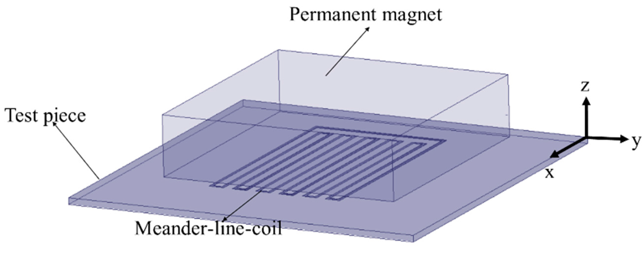
Previously, the authors have conducted EMAT modelling for Rayleigh waves focussing on the vertical plane of the material. This model combines the analytical method and FDTD to model EMATs [15]. The dimension and material of the test piece, the coil, and the permanent magnet are the same as the ones used in [15] by Xie et al. Based on such design, the working frequency used to form the interference of Rayleigh waves is 483 kHz.

2.1. EMAT-EM Model

This section introduces the EMAT-EM model to analyse the distribution of $\mathbf{F}$ (Lorentz force density). Firstly, the classic Dodd and Deeds solution [20] to the vector potential is described, and the strategy of adapting the circular analytical solutions for a straight wire is introduced (Section 2.1.1). The FEM is employed to validate the adapted solution (Section 2.1.2). Finally, based on the adapted analytical solutions, the distribution of Lorentz force density is presented (Section 2.1.3).

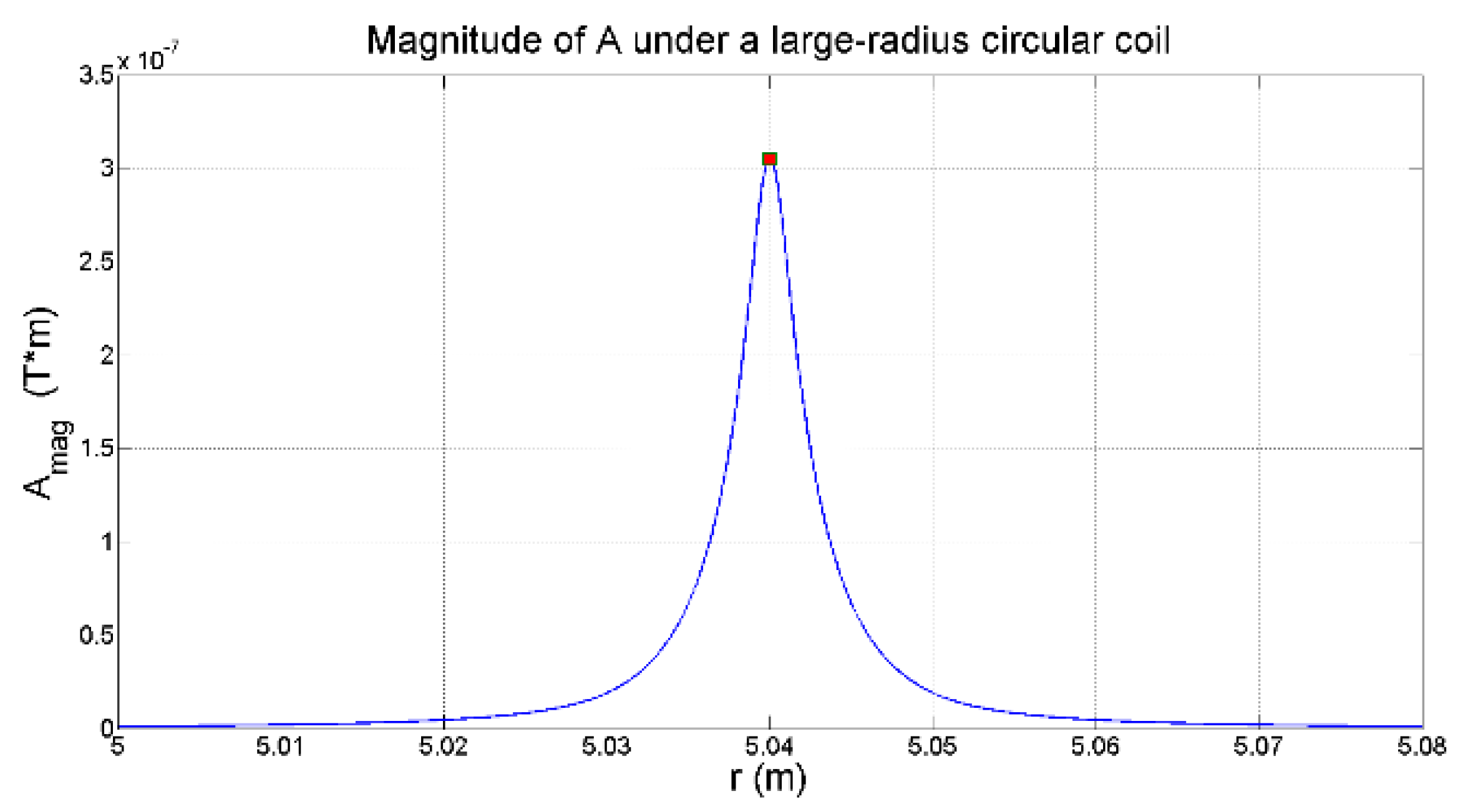
2.1.1. Adapted Analytical Solutions to the Vector Potential for a Straight Wire

The governing equations for calculating eddy currents are described in Equations (2)–(4):

$${\nabla }^2\mathbf{A}=-\mu \mathbf{I}+\mu \sigma \frac{\partial \mathbf{A}}{\partial t}+\mu \epsilon \frac{{\partial }^2\mathbf{A}}{\partial t^2}+\mu \nabla (\frac{1}{\mu })\times (\nabla \times \mathbf{A})$$

(2)

$$\mathbf{E}=-j\omega \mathbf{A}$$

(3)

$$\mathbf{J}=\sigma \mathbf{E}$$

(4)

where A is the vector potential generated by I, ω and I are the angular frequency and the density of the applied alternating current (AC), respectively, ε, µ and σ are the permittivity, permeability and conductivity of the test piece respectively, and E and J are the induced electric field and eddy current density, respectively [20].

As described in [15] by Xie et al., for a small radius circular coil, the distribution of the vector potential A at z = 0 (surface of the sample) is not symmetrical with the radius due to the bent wire.

The coil used in this work consists of straight wires; thus, the analytical solution for a straight wire is needed. The adapted solution for a straight wire has been presented in [15] by Xie et al. Here is a brief introduction. A hypothesis is proposed: if the radius of the circular coil, compared with its width, is very large, a bent wire can be viewed as a straight wire, and the distribution of A should be symmetrical. To validate such a hypothesis, a model is built with a large-radius circular coil above the aluminium plate. The aluminium sample used has a dimension of 80 mm × 30 mm, and the inner radius and the outer radius of the circular coil are set to 5.0395 m and 5.0405 m, respectively. At 1 kHz, the current density applied to the circular coil is 1 A/m², and the lift-off of the coil is 1 mm. The permeability and the conductivity of the aluminium plate are 1.257 × 10⁻⁶ H/m and 3.8 × 10⁷ Siemens/m, respectively.

The distribution of the magnitude of A based on the adapted solution is shown in Figure 2. The red marker denotes the maximum magnitude of the vector potential. The distribution of the magnitude of A is symmetrical with the radius of 5.04 m, where the coil is located. The result verifies the hypothesis that, when the radius of the circular coil is very large, a bent wire serves as a straight wire.

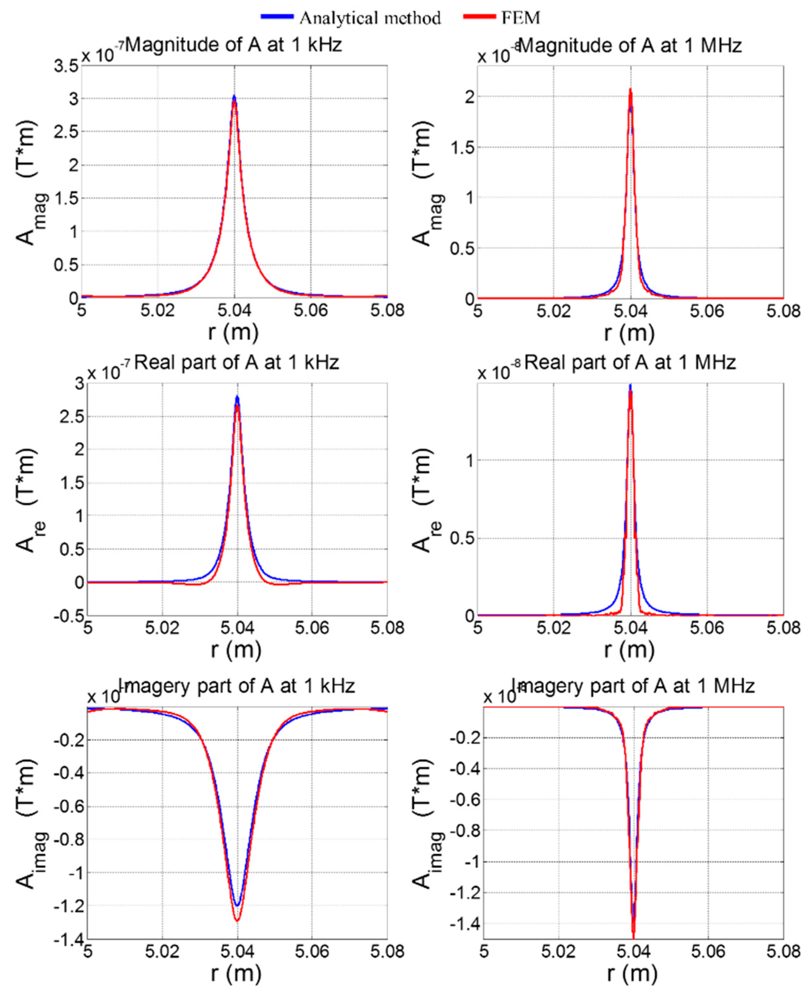
2.1.2. Comparison between the Adapted Solution and FEM

In order to compare the adapted solutions to FEM, Maxwell Ansoft, which is a FE solver, is utilised. The FEM model has a rectangular cross-sectional coil located above the cross-sectional aluminium plate, and is surrounded by a vacuum region that is four times larger than the sample. The FEM subdivides the large model to smaller elements, and this FEM solves the calculation by minimising the energy error. In this work, when the elements number is beyond 20,000, the energy error is as low as 0.05%, which is sufficiently accurate for the FEM computation. In this work, the mesh number used is 20,395, and the boundary used is a balloon boundary to simulate an infinite space. The distribution of A at the sample’s surface (z = 0) is presented in Figure 3. The analytical solution and FEM present a good agreement at an operational frequency of 1 kHz. However, at a working frequency of 1 MHz, the distribution of A from the FEM is not smooth compared to that from the analytical solution; the reason is that the FEM is affected by the elements density and numerical approximation is unavoidable, etc. Therefore, the adapted analytical method presents a more accurate result compared to FEM, especially for a high working frequency.

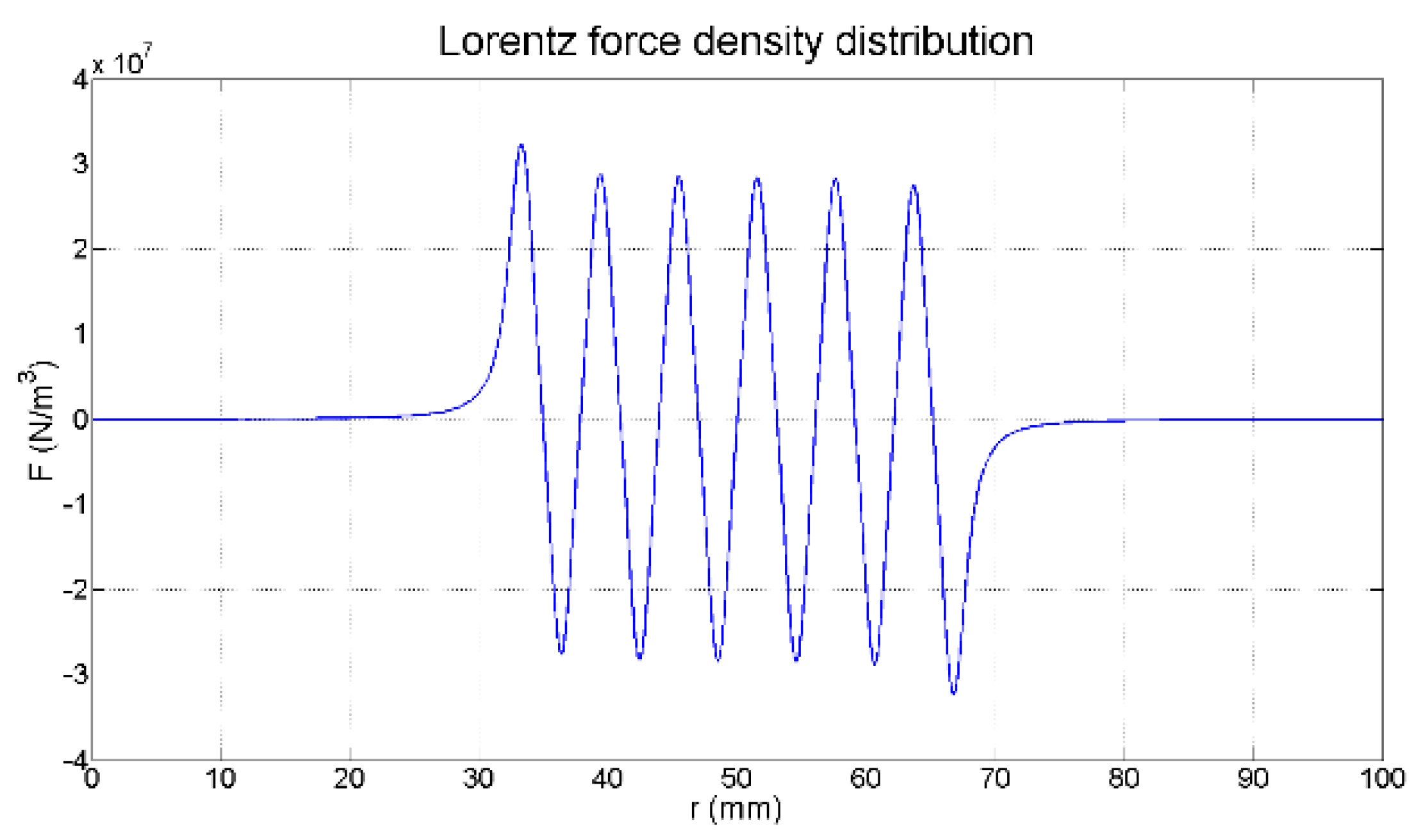
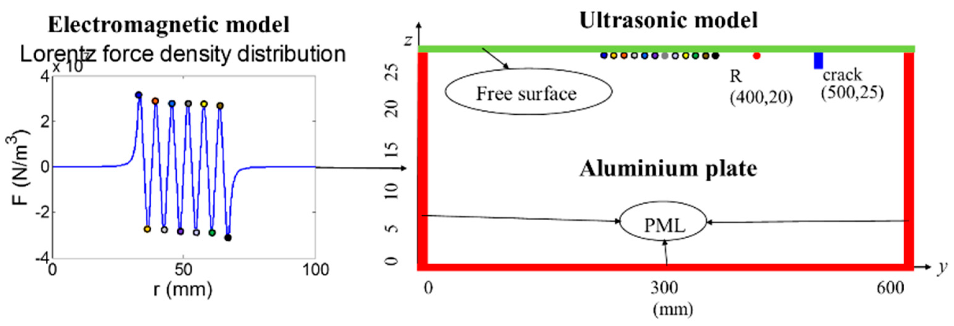
2.1.3. EMAT-Lorentz Force Calculation

The analytical solution to a straight wire has been described in Section 2.1.2. A (vector potential) generated by a meander-line-coil is the addition of A generated by every single straight wire. The zone where the meander-line-coil mainly operates on is selected to model EM simulation to increase the modelling effectiveness. The distribution of A and F at z = 0 are shown in Figure 4 and Figure 5. The generated periodic fields have different directions for any neighbouring wires, since their applied ACs are opposite, and therefore, the periodic distribution of A and F has six positive values and six negative values. The outermost A and outermost F are largest, because A is under the outermost wires, and thus is only determined by the fields on one side.

2.2. EMAT-US Simulation

2.2.1. Elastodynamic Equations

Elastodynamic equations (Equations (5) and (6)) are a group of partial differential equations to model the wave propagation:

$$\rho (x)\frac{\partial v_i}{\partial \mathrm{t}}(x,t)={\sum }_{j=1}^d\frac{\partial {\mathit{T}}_{\mathit{i}\mathit{j}}}{\partial x_j}(x,t)+{\mathit{f}}_{\mathit{i}}(x,t)$$

(5)

$$\frac{\partial {\mathit{T}}_{\mathit{i}}}{\partial \mathrm{t}}={\sum }_{j=1}^d{\sum }_{i=1}^d{c}_{ijkl}(x)\frac{\partial v_k}{\partial x_l}+{\mathit{\theta }}_{\mathit{i}\mathit{j}}(x,t)$$

(6)

where $\rho$ and $c_{ijkl}$ are the density and the fourth stiffness tensor of the material, and ${\mathit{f}}_{\mathit{i}}$ and ${\mathit{\theta }}_{\mathit{i}\mathit{j}}$ are the force source and strain tensor rate source, respectively.

2.2.2. Combination of EMAT-EM and EMAT-US Models

As described in Section 2.1.3, F is obtained from the EMAT-EM calculation. In this section, F, which is used as the force source, is imported to the EMAT-US model to produce ultrasound (Figure 6). Since F is calculated in the frequency domain and FDTD is a time-domain solver, the excitation signal for the EMAT-US model is a time sequence signal with the peak equalling the peak values of F. The excitation signal used is a Gaussian-modulated sinusoidal with a fractional width of 0.18. A crack and a receiver R are located within the sample, as shown in Figure 6. Regarding the FDTD setup in the ultrasonic model, there are two main parameters: the spatial step, and the time step. The spatial step used is 0.2 mm, which approximately equals to 1/30th of the wavelength. The time step is 0.0222 µs, which is calculated based on the Courant–Friedrichs–Lewy (CFL) condition. Free surface conditions are utilised on the surface of the sample. Perfectly-matched layers (PML) with a thickness of 16 mm are utilised to absorb ultrasound.

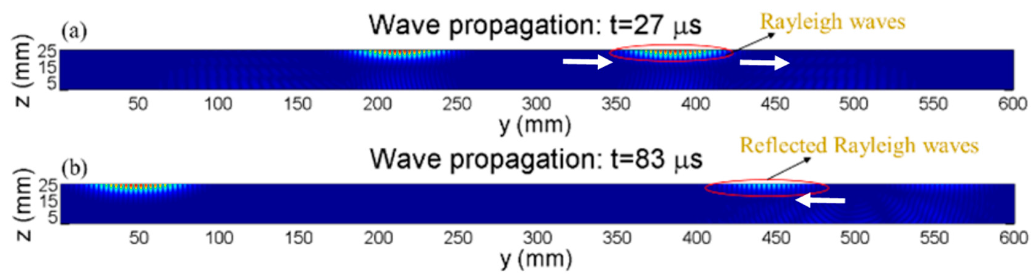
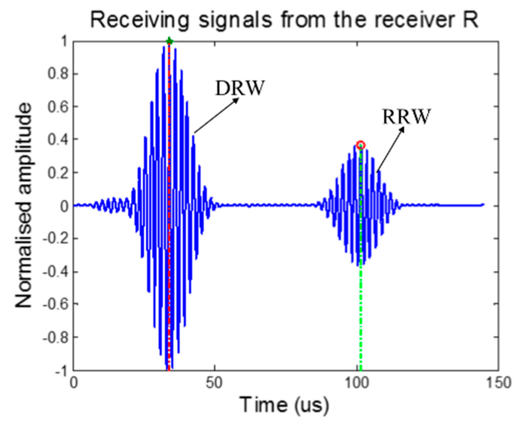
2.2.3. Wave Propagations

Based on FDTD calculations, the velocity fields of ultrasound waves are obtained. The velocity fields at 27 µs and 83 µs are shown in Figure 7, which describes the Rayleigh waves’ propagation and their scattering behaviours, respectively. The white arrows denote the propagation path.

2.3. EMAT-Reception Simulation

The EMAT reception process has been reported quite a lot [21]. The received signal from simulations is shown in Figure 8, where DRW and RRW denote the directly transmitted Rayleigh waves and the reflected Rayleigh waves, respectively. The propagation distance of DRW and RRW is 100 mm and 300 mm, respectively, and the velocity of Rayleigh waves is 2.93 mm/µs; hence, the theoretically arrival time of DRW and RRW is 34 µs and 102.4 µs, respectively. Figure 8 shows the numerically arrival time of DRW and RRW; these numerical and experimental results present a good agreement.

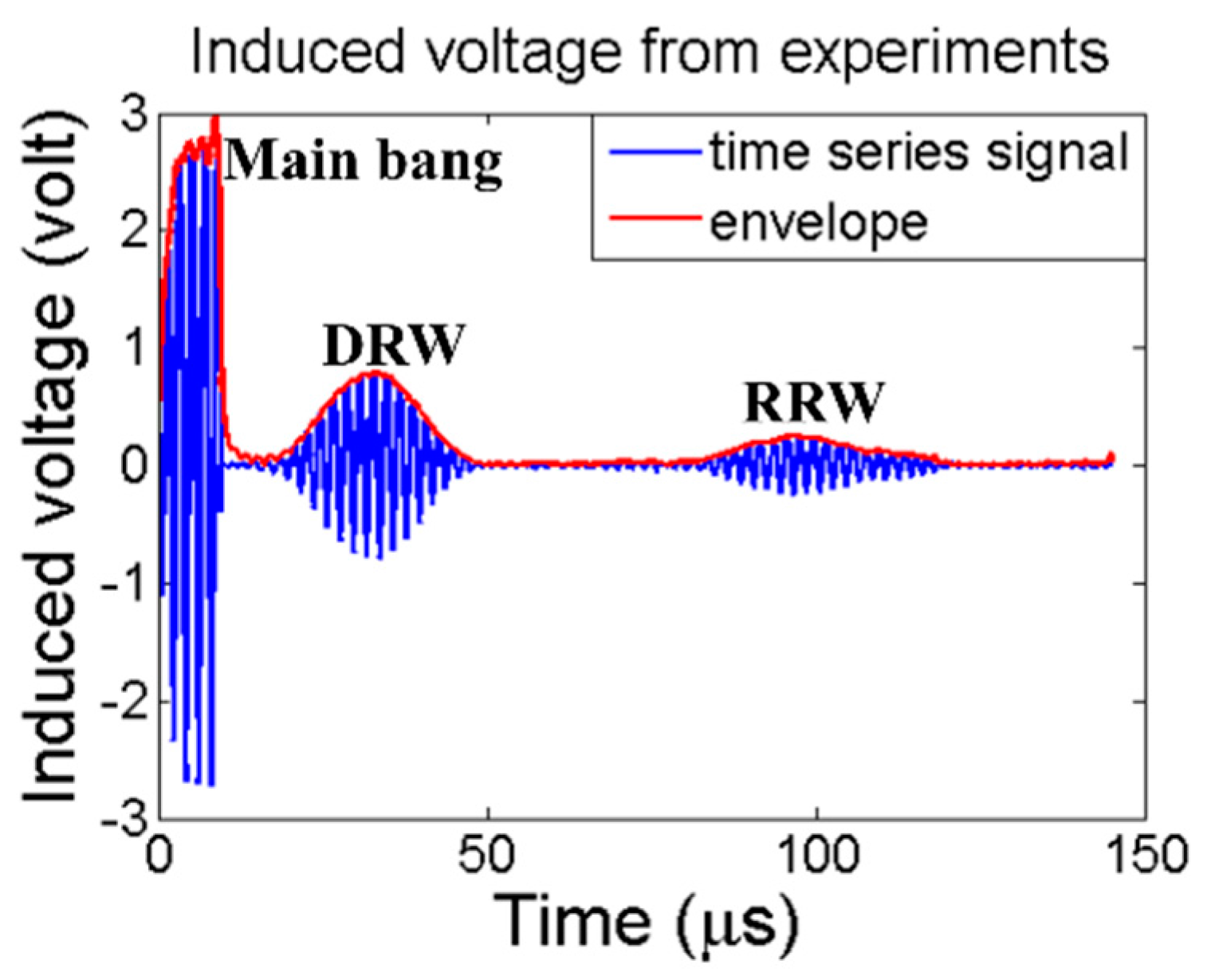
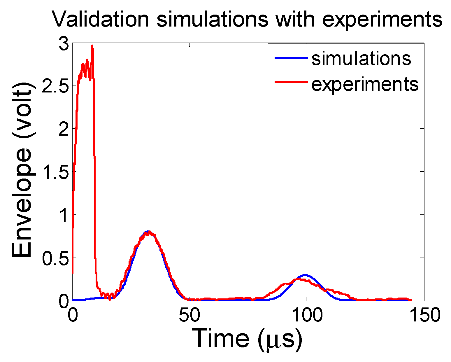
2.4. Experimental Validations

Experiments were carried out to validate the proposed modelling method. The setup of the experiments is the same as that of our previous work [15]. The received signals from experiments are shown in Figure 9, where three signals are observed. The “Main bang” is the interference signal due to a high power excitation, arriving before DRW and RRW. The red curve and the blue curve are the envelope and the time series signal, respectively.

Figure 10 shows the envelope of DRW and RRW from experiments and simulations. The experimental arrival times of DRW is 34 µs, which is consistent with the numerical results. However, the experimental arrival time of RRW is slightly different from the simulations. This is because of the approximated model used and the inevitable experimental noise.

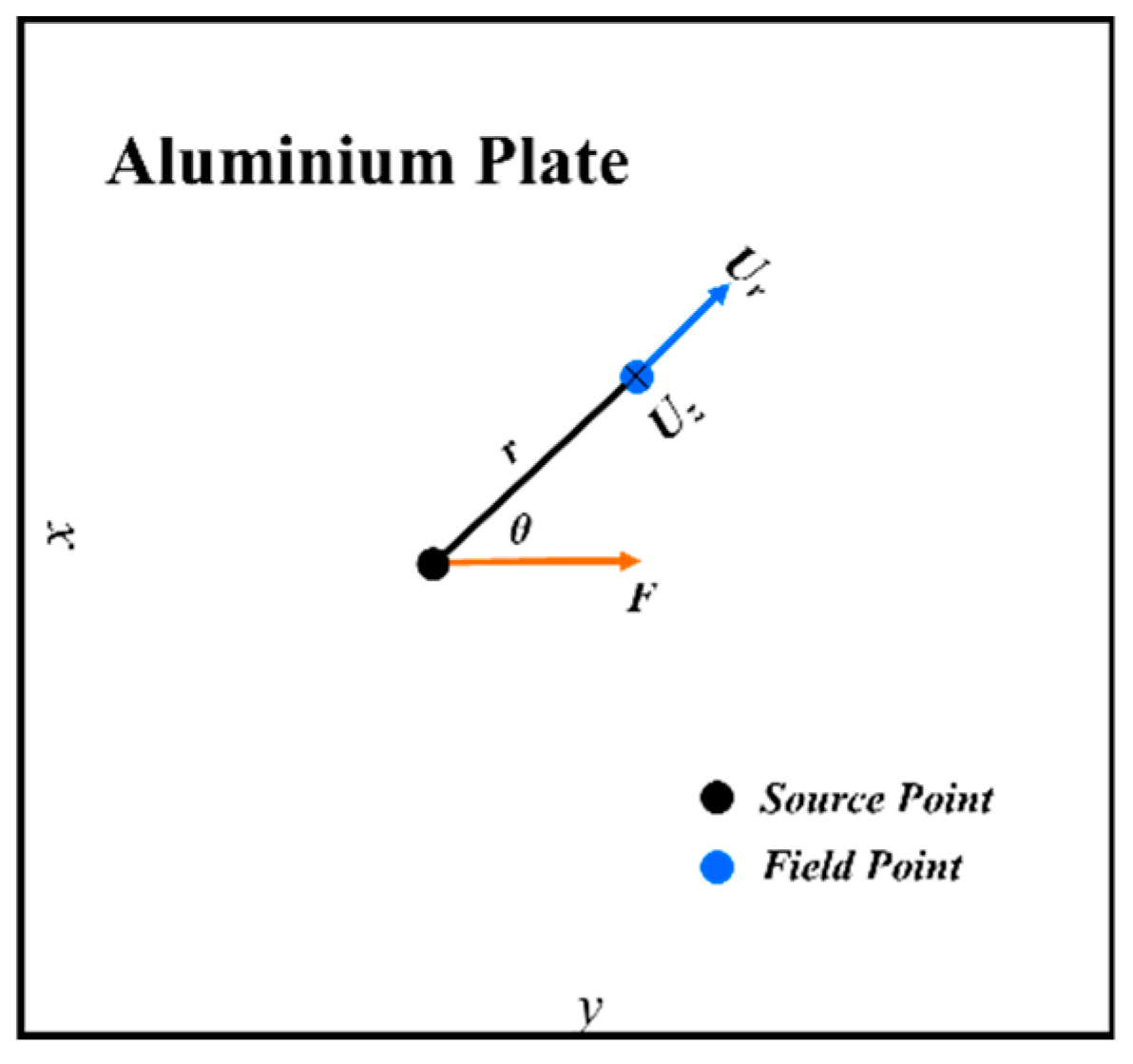
3. Horizontal Surface Plane Modelling—Directivity Analysis of Rayleigh Waves

The main mode of propagation on the horizontal surface of the material is the Rayleigh wave. The radiation pattern and the beam directivity of Rayleigh waves at z = 0 (Figure 1) were reported in [18] by Xie et al. Rayleigh waves not only distribute along the surface (z = 0), they also distribute within a depth of the Rayleigh waves’ wavelengths. However, Rayleigh waves not only concentrate on the surface, they also concentrate within a depth of one wavelength. In this section, the beam directivity of Rayleigh waves at various depths are investigated utilising an analytical method.

3.1. The Analytical Solution to the Displacement of Rayleigh Waves

N. A. Haskell proposed an analytical solution to Rayleigh waves [22,23]. Ref. [24] by Love introduced these solutions in detail, and investigated the beam directivity of Rayleigh waves at z = 0 with approximated equations. However, Rayleigh waves not only concentrate on the surface; they also concentrate within a depth of one wavelength. The complete equations of the Rayleigh waves’ displacement at various depths are:

$${\mathit{u}}_{\mathit{r}}=A(\mathsf{ĸ},r,z)e^{-\frac{\pi i}{4}}\frac{2\mathsf{ĸ}(\gamma -1)}{v_{\beta }}\mathit{F}(\frac{2}{\gamma }-1+\frac{\gamma -1}{\gamma }{e}^{-z(v_{\alpha }-v_{\beta })})$$

(7)

$${\mathit{u}}_{\mathit{z}}=\frac{i\gamma v_{\alpha }{\mathit{u}}_{\mathit{r}}}{\mathsf{ĸ}(\gamma -1)}$$

(8)

where:

$$A(\mathsf{ĸ},r,z)=\frac{{\mathsf{ĸ}}^2\gamma v_{\beta }}{4\rho (\frac{2{\gamma }^2{v}_{\alpha }{v}_{\beta }}{{\mathsf{ĸ}}^3})}\sqrt{\frac{2}{\pi \mathsf{ĸ}r}}{e}^{(-i\mathsf{ĸ}r-z{v}_{\beta })}$$

(9)

$$\gamma =\cos (\theta )$$

(10)

$$v_{\alpha }=\{\begin{array}{ll}\sqrt{{\mathsf{ĸ}}^2-{(\omega /c_L)}^2}& \mathsf{ĸ}>\omega /c_L\\ i\sqrt{{(\omega /c_L)}^2-{\mathsf{ĸ}}^2}& \mathsf{ĸ}<\omega /c_L\end{array}$$

(11)

$$v_{\beta }=\{\begin{array}{ll}\sqrt{{\mathsf{ĸ}}^2-{(\omega /c_S)}^2}& \mathsf{ĸ}>\omega /c_s\\ i\sqrt{{(\omega /c_S)}^2-{\mathsf{ĸ}}^2}& \mathsf{ĸ}<\omega /c_s\end{array}$$

(12)

$$\mathsf{ĸ}=\frac{\omega }{c_R}$$

(13)

where ${\mathit{u}}_{\mathit{r}}$ and ${\mathit{u}}_{\mathit{z}}$ are the in-plane and the out-of-plane displacement to be calculated, respectively; $r$ is the distance between the source point and the field point (Figure 11); $\mathit{F}$ is the excitation source; $\rho$ is the density of the material; $\theta$ is the angle between the force vector and the in-plane displacement vector; $\omega$ is the operational angular frequency; z is the depth; and $c_L$, $c_S$, $c_R$, and $\mathsf{ĸ}$ are the velocity of the longitudinal waves, shear waves, Rayleigh waves, and the wave number, respectively.

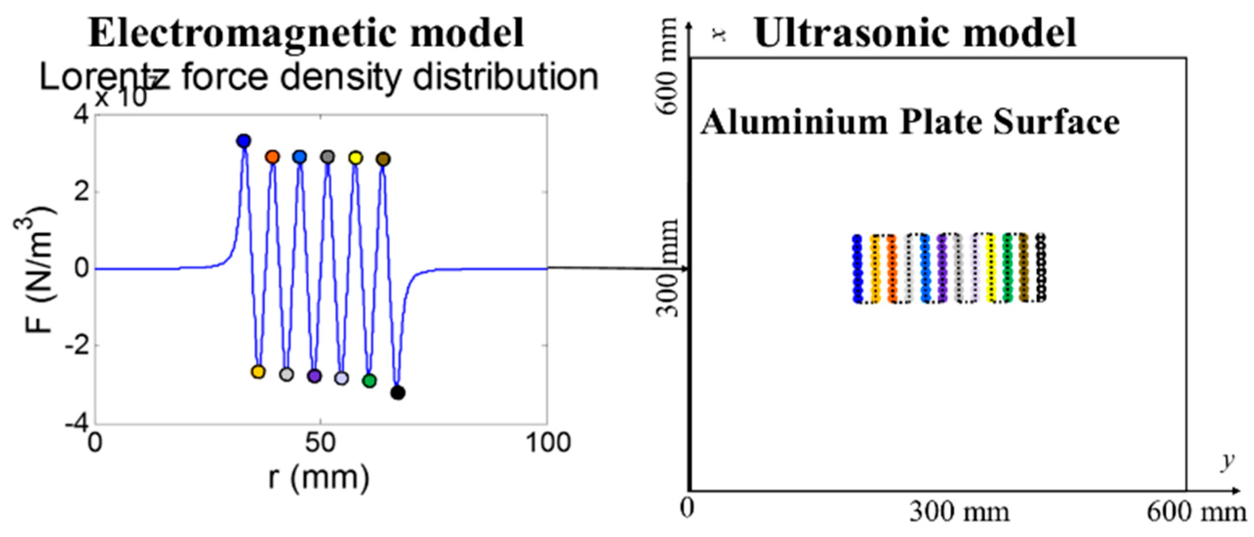
3.2. Linking EMAT-EM and EMAT-US Models

On the surface plane of the material, the combination between the EMAT-EM model and the EMAT-US model is described in Figure 12. The calculated F values, acting as the excitation source, are imported to each surface layer at various depths. The Rayleigh waves’ distribution is the addition of the Rayleigh waves generated by each point source.

Table 1. Detailed parameters used for the EMAT-US modelling.

Description	Symbol	Value
Length of the aluminium plate	Y	600 mm
Width of the aluminium plate	X	600 mm
Field spatial step	∆xf	1 mm
Length of the meander-line-coil	L	50 mm
Source spatial step for each wire	∆xs	0.2 mm
Density of the aluminium plate	ρ	2700 kg/m3
Frequency	f	483 kHz
Longitudinal waves’ velocity	Cl	6.375 mm/$\mathsf{\mu }\mathrm{s}$
Shear waves’ velocity	Cs	3.14 mm/$\mathsf{\mu }\mathrm{s}$
Rayleigh waves’ velocity	Cr	2.93 mm/$\mathsf{\mu }\mathrm{s}$

illustrates the parameters used for the EMAT-US model.

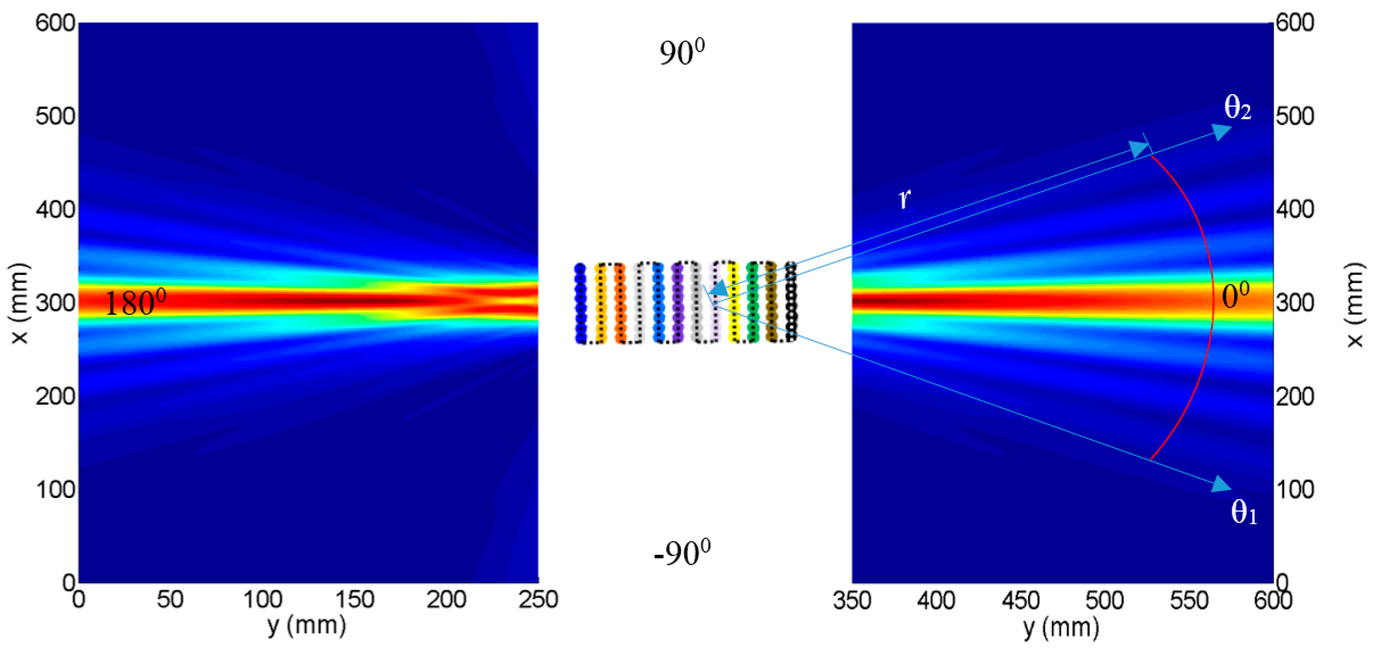
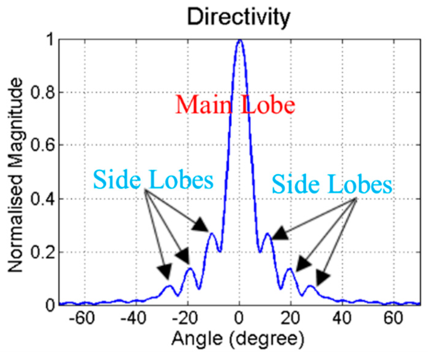
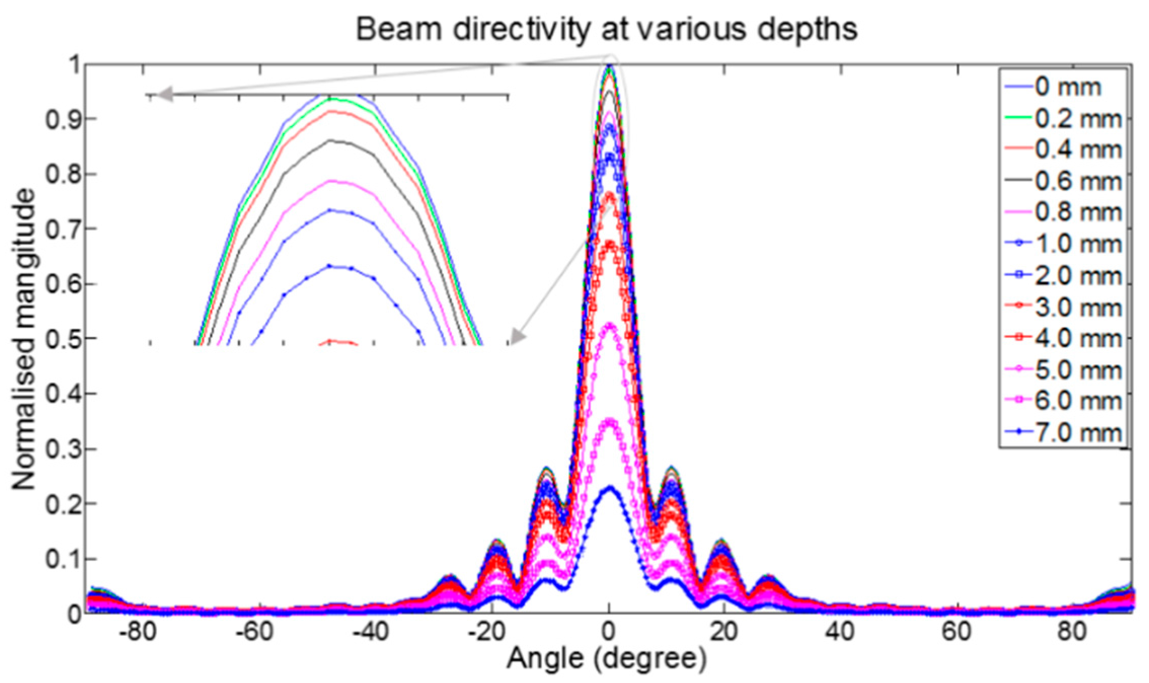
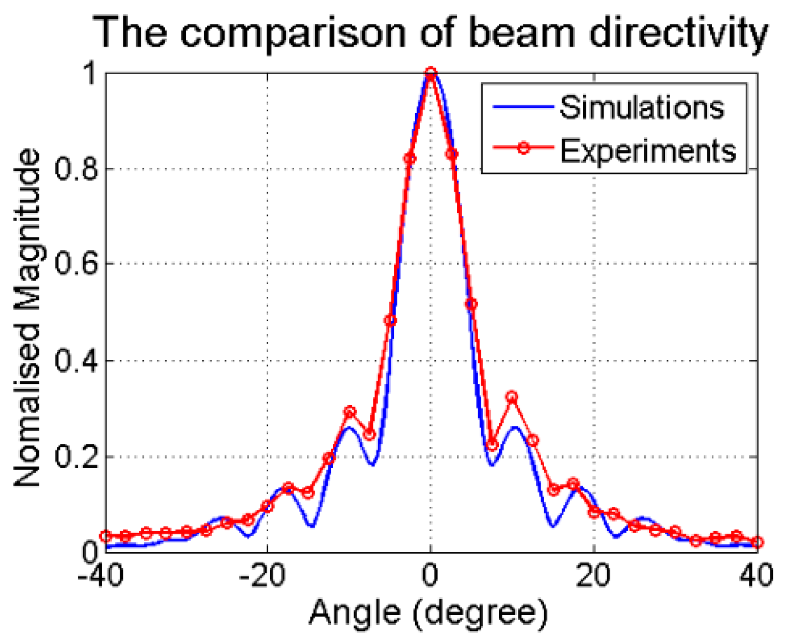
3.3. Analysis of the Beam Directivity of Rayleigh Waves

Figure 13 shows the calculated Rayleigh waves’ radiation pattern at z = 0, which is symmetrical with the center of the coil. Rayleigh waves are mainly generated along the y direction (main lobe) and some undeniable directions (side lobe). The characteristics of Rayleigh waves are quantitatively investigated by means of beam directivity, as shown in the red arc in Figure 13 (r = 250 mm, θ₁ = −70°, and θ₂ = 70°).

The beam directivity of Rayleigh waves at z = 0 is shown in Figure 14. A main lobe contains a larger magnitude compared to the side lobes, which contain a smaller magnitude. The main lobe is centered at 0°, and the side lobes are roughly centered at −25.5°, −18°, −10°, 10°, 18°, and 25.5°, respectively. The largest magnitude of the side lobes is 25.87% that of the main lobe. In most applications, side lobes are usually undesirable.

The beam directivity of the Rayleigh waves at various depths is shown in Figure 15. The magnitude of the beam directivity is normalised. From this image, the magnitude of the Rayleigh waves decays with the depth, especially for the depth larger than one Rayleigh wavelength. At a depth equalling to one Rayleigh wave’s wavelength, z = 6 mm, the magnitude of the Rayleigh waves is 34.9% of that at z = 0. At a depth of 7 mm, the magnitude of the Rayleigh waves decays to 22.8% of that at the surface of the test piece (z = 0). This observation confirms that Rayleigh waves mainly distribute within a depth equal to one Rayleigh wavelength.

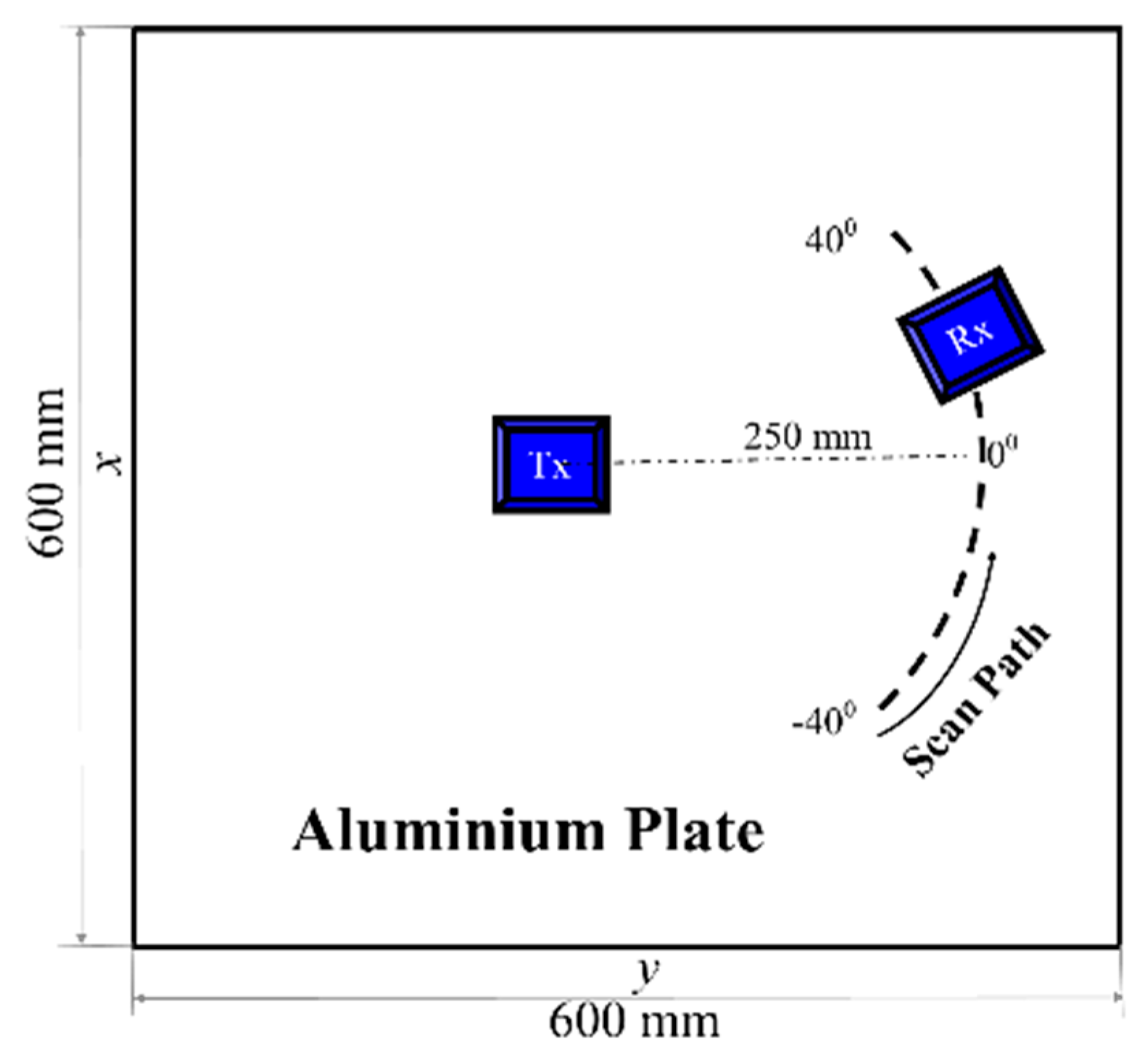
3.4. Experimental Validations

In Figure 15, based on the analytical simulations, the distribution of the Rayleigh waves at various depths is presented. In this part, the measured results at z = 0 are picked to compare with the simulation results. The experimental setup was the same as the one in Section 2.4. The measured beam directivity at z = 0 is obtained by placing the receiver along the scanning path, as shown in Figure 16. Figure 17 shows the beam directivity results at z = 0 from simulations and experiments. Thirty-three measuring points on the scanning path were picked with a moving step of 2.5°. The measured beam directivity at z = 0 agrees well with the simulated beam directivity, which validates the proposed method. There are some non-overlapping points between these two curves due to several factors, which include the experimental noise and the tolerance of the receiver’s position, etc.

4. Conclusions

A pseudo-3D model for simulating meander-line-coil EMATs was proposed. A method combining the analytical method for the EM model and FDTD for the US model was utilised to simulate the Rayleigh waves’ propagation. On the other hand, a wholly analytical method was utilised to simulate the radiation pattern of the Rayleigh waves. For both cases, analytical solutions to the EM model were adapted from the classic Dodd and Deeds solution in order to calculate eddy currents under straight wires. By comparing with the FEM, the analytical solutions are more accurate. Experiments were conducted in order to validate the proposed method, and these showed a good consistency. The beam directivity of Rayleigh waves at various depths were investigated, and results confirmed that Rayleigh waves mainly distribute within a depth of one wavelength of Rayleigh waves. Overall, this pseudo-3D model combines both the vertical plane and surface plane of EMAT models, and provides the beam directivity of Rayleigh waves at various depths, which have not been reported previously. Therefore, this work can be a starting point to build an advanced EMAT 3D model in the future. There are some limitations of the proposed 3D EMAT model. Firstly, it can only be applied in a homogeneous medium. It is worth investigating the 3D EMAT model for a multiple-layer medium, since multiple-layer samples are widely used in applicable industries. Secondly, the EMAT-US model on the vertical plane of the sample uses an approximated model with only point sources (Lorentz force density) to generate Rayleigh waves. A more detailed model with volume sources within the skin depth is worth considering in the future. In addition, it is worth investigating the scattering behaviours of defects in other orientations, as it is a variable in practical application.

References

1. Buchner, S.P.; Miller, F.; Pouget, V.; McMorrow, D.P. Pulsed-laser testing for single-event effects investigations. IEEE Trans. Nucl. Sci. 2013, 60, 1852–1875. [Google Scholar] [CrossRef]
2. Taheri, H.; Delfanian, F.; Du, J. Ultrasonic phased array techniques for composite material evaluation. J. Acoust. Soc. Am. 2013, 134, 4013. [Google Scholar] [CrossRef]
3. Yin, W.; Dickinson, S.; Peyton, A. A multi-frequency impedance analysing instrument for eddy current testing. Meas. Sci. Technol. 2006, 17, 393. [Google Scholar] [CrossRef]
4. Yin, W.; Peyton, A.J.; Dickinson, S.J. Simultaneous measurement of distance and thickness of a thin metal plate with an electromagnetic sensor using a simplified model. IEEE Trans. Instrum. Meas. 2004, 53, 1335–1338. [Google Scholar] [CrossRef]
5. Dixon, S.; Edwards, C.; Palmer, S. High accuracy non-contact ultrasonic thickness gauging of aluminium sheet using electromagnetic acoustic transducers. Ultrasonics 2001, 39, 445–453. [Google Scholar] [CrossRef]
6. Edwards, R.S.; Dixon, S.; Jian, X. Non-contact ultrasonic characterization of defects using EMATs. AIP Conf. Proc. 2005, 760, 1568. [Google Scholar]
7. Edwards, R.S.; Sophian, A.; Dixon, S.; Tian, G.-Y.; Jian, X. Dual EMAT and PEC non-contact probe: Applications to defect testing. NDT E Int. 2006, 39, 45–52. [Google Scholar] [CrossRef]
8. Hutchins, D.; Schindel, D. Advances in non-contact and air-coupled transducers (US materials inspection). In Proceedings of the Ultrasonics Symposium, Cannes, France, 31 October–3 November 1994; IEEE: Piscataway, NJ, USA, 1994. [Google Scholar]
9. Hirao, M.; Ogi, H. EMATs for Science and Industry: Noncontacting Ultrasonic Measurements, 1st ed.; Springer Science & Business Media: New York, NY, USA, 2003; 372p. [Google Scholar]
10. Jian, X.; Dixon, S.; Grattan, K.T.V.; Edwards, R.S. A model for pulsed Rayleigh wave and optimal EMAT design. Sens. Actuators A Phys. 2006, 128, 296–304. [Google Scholar] [CrossRef]
11. Wang, S.; Kang, L.; Li, Z.; Zhai, G.; Zhang, L. A novel method for modeling and analysis of meander-line-coil surface wave EMATs. In Life System Modeling and Intelligent Computing; Kang, L., Fei, M., Jia, L., Irwin, G.W., Eds.; Springer: Berlin/Heidelberg, Germany, 2010; pp. 467–474. [Google Scholar]
12. Kang, L.; Dixon, S.; Wang, K.; Dai, J. Enhancement of signal amplitude of surface wave EMATs based on 3-D simulation analysis and orthogonal test method. NDT E Int. 2013, 59, 11–17. [Google Scholar] [CrossRef]
13. Dhayalan, R.; Balasubramaniam, K. A hybrid finite element model for simulation of electromagnetic acoustic transducer (EMAT) based plate waves. NDT E Int. 2010, 43, 519–526. [Google Scholar] [CrossRef]
14. Dhayalan, R.; Balasubramaniam, K. A two-stage finite element model of a meander coil electromagnetic acoustic transducer transmitter. Nondestruct. Test. Eval. 2011, 26, 101–118. [Google Scholar] [CrossRef]
15. Xie, Y.; Rodriguez, D.S.; Yin, W.; Peyton, A.; Liu, Z.; Hao, J.; Zhao, Q.; Wang, B. Simulation and experimental verification of a meander-line-coil electromagnetic acoustic transducers (EMATs). In Proceedings of the Instrumentation and Measurement Technology Conference (I2MTC), Taipei, Taiwan, 23–26 May 2016; IEEE International: Piscataway, NJ, USA, 2016. [Google Scholar]
16. Xie, Y.; Yin, L.; Rodriguez, S.G.; Yang, T.; Liu, Z.; Yin, W. A wholly analytical method for the simulation of an electromagnetic acoustic transducer array. Int. J. Appl. Electromagn. Mech. 2016, 51, 1–15, (Preprint). [Google Scholar] [CrossRef]
17. Xie, Y.; Yin, W.; Liu, Z.; Peyton, A. Simulation of ultrasonic and EMAT arrays using FEM and FDTD. Ultrasonics 2016, 66, 154–165. [Google Scholar] [CrossRef] [PubMed]
18. Xie, Y.; Liu, Z.; Yin, L.; Wu, J.; Deng, P.; Yin, W. Directivity analysis of Meander-Line-Coil EMATs with a wholly analytical method. Ultrasonics 2017, 73, 262–270. [Google Scholar] [CrossRef] [PubMed]
19. Wang, S.; Kang, L.; Li, Z.; Zhai, G.; Zhang, L. 3-D modeling and analysis of meander-line-coil surface wave EMATs. Mechatronics 2012, 22, 653–660. [Google Scholar] [CrossRef]
20. Dodd, C.; Deeds, W. Analytical Solutions to Eddy-Current Probe-Coil Problems. J. Appl. Phys. 1968, 39, 2829–2838. [Google Scholar] [CrossRef]
21. Jian, X.; Dixon, S.; Quirk, K.; Grattan, K.T.V. Electromagnetic acoustic transducers for in-and out-of plane ultrasonic wave detection. Sens. Actuators A Phys. 2008, 148, 51–56. [Google Scholar] [CrossRef]
22. Haskell, N. Radiation pattern of Rayleigh waves from a fault of arbitrary dip and direction of motion in a homogeneous medium. Bull. Seismol. Soc. Am. 1963, 53, 619–642. [Google Scholar]
23. Haskell, N. Radiation pattern of surface waves from point sources in a multi-layered medium. Bull. Seismol. Soc. Am. 1964, 54, 377–393. [Google Scholar]
24. Love, A.E.H. A Treatise on the Mathematical Theory of Elasticity; Dover Publication: New York, NY, USA, 1944; 643p. [Google Scholar]
Figure 1. The configuration of a typical meander-line-coil electromagnetic acoustic transducer (EMAT). Reproduced with permission from [15], IEEE, 2016.
Applsci 08 00450 g001
Figure 2. The magnitude distribution of A under a large-radius circular coil. Reproduced with permission from [15], IEEE, 2016.
Applsci 08 00450 g002
Figure 3. The distribution of A from the adapted analytical solution and the finite element method (FEM). The left curves are the results at 1 kHz, while the right curves are the results at 1 MHz. The red curve is the result from the FEM, and the blue curve is the result from the analytical solutions. Reproduced with permission from [15], IEEE, 2016.
Applsci 08 00450 g003
Figure 4. For a meander-line-coil, the distribution of the vector potential A at z = 0. Reproduced with permission from [15], IEEE, 2016.
Applsci 08 00450 g004
Figure 5. For a meander-line-coil, the distribution of the Lorentz force density F at z = 0. Reproduced with permission from [15], IEEE, 2016.
Applsci 08 00450 g005
Figure 6. On the vertical plane of the material, the combination of the EMAT-electromagnetic (EM) and EMAT-ultrasonic (US) models. Reproduced with permission from [15], IEEE, 2016.
Applsci 08 00450 g006
Figure 7. Wave propagations. (a,b) denote the velocity fields at 27 µs and 83 µs, respectively. Reproduced with permission from [15], IEEE, 2016.
Applsci 08 00450 g007
Figure 8. The received signal from simulations. Reproduced with permission from [15], IEEE, 2016.
Applsci 08 00450 g008
Figure 9. The received signal from experiments. The blue curve denotes the induced voltage in the received coil, and the red curve denotes the envelope of the received signal. Reproduced with permission from [15], IEEE, 2016.
Applsci 08 00450 g009
Figure 10. The envelope of the received signals. The blue curve and the red curve are the envelope of the received signal from simulations and experiments, respectively.
Applsci 08 00450 g010
Figure 11. The model used to simulate Rayleigh waves. Reproduced with permission from [18], Elsevier, 2017.
Applsci 08 00450 g011
Figure 12. On the surface plane of the material, the transformation between the EM and US models. Reproduced with permission from [18], Elsevier, 2017.
Applsci 08 00450 g012
Figure 13. The radiation pattern of Rayleigh waves generated by the meander-line-coil EMAT. Reproduced with permission from [18], Elsevier, 2017.
Applsci 08 00450 g013
Figure 14. The simulated beam directivity of Rayleigh waves at z = 0. Reproduced with permission from [15], IEEE, 2016.
Applsci 08 00450 g014
Figure 15. The simulated beam directivity of Rayleigh waves at various depths.
Applsci 08 00450 g015
Figure 16. The scanning path of the receiver.
Applsci 08 00450 g016
Figure 17. The comparison between the simulated beam directivity and the experimental beam directivity at z = 0. The red curve is the beam directivity from simulations, while the blue curve is the beam directivity from experiments.
Applsci 08 00450 g017