Ensemble Classification of Data Streams Based on Attribute Reduction and a Sliding Window

Featured Application

The proposed ensemble classification algorithm can be applied in areas such as network analysis or target identification, especially in the field of sensor network monitoring.

Abstract

With the current increasing volume and dimensionality of data, traditional data classification algorithms are unable to satisfy the demands of practical classification applications of data streams. To deal with noise and concept drift in data streams, we propose an ensemble classification algorithm based on attribute reduction and a sliding window in this paper. Using mutual information, an approximate attribute reduction algorithm based on rough sets is used to reduce data dimensionality and increase the diversity of reduced results in the algorithm. A double-threshold concept drift detection method and a three-stage sliding window control strategy are introduced to improve the performance of the algorithm when dealing with both noise and concept drift. The classification precision is further improved by updating the base classifiers and their nonlinear weights. Experiments on synthetic datasets and actual datasets demonstrate the performance of the algorithm in terms of classification precision, memory use, and time efficiency.

1. Introduction

With the emerging era of Big Data, data stream classification technology has become a main topic in data mining research. Data streams are massive, extremely long, and noisy, which make traditional data mining algorithms unable to satisfy the demands of practical applications such as network analysis or target identification. In addition, concept drift, caused by the hidden concept changing in data streams, poses great challenges to classifying data streams.

Recent studies mainly employ two types of methods to realize the classification of data streams, which are single classifier learning and ensemble classifier learning [1,2]. An ensemble classifier usually performs better than a single classifier [2,3]. The streaming ensemble algorithm was first introduced in Reference [4] to deal with concept drift in data stream classification by updating the base classifiers. The accuracy weighted ensemble (AWE) algorithm was further proposed [3] to weight base classifiers according to the classification error rate. The accuracy update ensemble algorithm [5] is based on nonlinear weights of the base classifiers and achieves higher precision and lower memory use than AWE. In Reference [2], one linear function and one nonlinear function are used to weight base classifiers when input data are added under different conditions.

In order to detect concept drift and improve the classification precision further, variable sliding windows are used in Reference [6] to capture the occurrence of concept drift including dealing with sudden concept drift using smaller windows and speeding up data processing of stable streams using larger windows. Concept drift is perceived by detecting the change in classification precision. However, false concept drift, which is caused by noise, can cause unnecessary updating of the base classifiers and can waste resources. In References [7,8,9], the concept drift detection method based on double thresholds can effectively decrease the influence of noise. In Reference [8], the method of comparing the data classification error rate of adjacent windows can detect sudden concept drift. In Reference [9], the method of comparing the minimum values of the classification error rate for each window further improves the detection efficiency of gradual concept drift.

In addition, using attribute reduction or other dimension reduction methods to improve execution speed has become a key topic in the research of data stream processing. In Reference [2], the number of base classifiers is set to maximum and increased or decreased under different conditions, which saves memory demand. In Reference [10], the classification error rate of each attribute is compared to select important attributes. In Reference [11], the attribute reduction algorithm based on rough sets reduces the computation complexity sufficiently by relaxing the measurement criteria of attribute importance and ensures the distinctiveness of the reduced data using a specific strategy. However, this algorithm uses an attribute importance measure based on the positive region, which is defined as the union of lower approximations. Compared with an attribute reduction algorithm based on information entropy, it deals with system uncertainty poorly [12]. Meanwhile, the difference between base classifiers is the key factor that affects the overall performance of an ensemble system [11] and perturbing the sample attribute space by attribute reduction has become the main approach to increase this difference [13,14].

In this paper, we propose an ensemble classification algorithm of data streams based on attribute reduction and a sliding window. In the algorithm, we use double thresholds to detect concept drift and update the sliding window size. We use the data attributes after reduction and nonlinear weights of base classifiers to improve the data classification precision of noisy data streams. Our work in this paper consists of three main parts. Using mutual information, we propose a rough set-based approximate attribute reduction algorithm to decrease the computation complexity of the ensemble classification algorithm and increase the difference between base classifiers. By introducing the sliding window idea of congestion control in the transport layer of a computer network, we propose a size control strategy of sliding windows. A double-threshold concept drift detection method is proposed based on the size control strategy. Based on attribute reduction and the sliding window, we propose an ensemble classification algorithm of noisy data streams to improve the classification precision with low complexity.

The remainder of this paper is organized as follows. Section 2 describes the problem that we aim to solve by our proposed algorithm in the paper. Section 3 describes the rough set-based approximate attribute reduction algorithm. Section 4 describes the detection method of concept drift. Section 5 describes the ensemble classification algorithm of data streams in detail. Section 6 verifies and analyzes the algorithm performance and Section 7 presents a summary of the study.

2. Problem Definition

For time stamp $t$, a data stream consists of a continuous sequence of instances: $\{x_1,x_2,\cdots ,x_{t-1},x_t,x_{t+1},\cdots \}$. Each instance ${\mathbf{x}}_t=(s_1^t,s_2^t,\cdots ,s_m^t,y^t)$ is a feature vector of $(m+1)$-dimensional attributes, which consists of ${\mathbf{s}}_t=(s_1^t,s_2^t,\cdots ,s_m^t)$ and a class label $y$. The data stream also can be seen as a sequence of sets $\mathbf{D}=\{\cdots ,d_{t-1},d_t,d_{t+1},\cdots \}$ where each element $d_t$ is a set of instances in a sliding window at time $t$.

In a data stream, the data distributions and definitions of target classes change over time. These changes are categorized into gradual or sudden concept drift depending on the appearance of novel classes in a stream and the rate of changing definitions of classes [15].

The aim of this paper is to present a high-performance ensemble classification algorithm of noisy data streams to improve the classification precision and sensitivity to concept drift with low computation complexity. At each time stamp $t$, the classification algorithm outputs a class prediction $y$ for each incoming instance.

3. Reduction of Data Streams

To reduce memory use and the processing time of the ensemble classification algorithm, we propose an approximate attribute reduction algorithm in this paper. The approximate attribute reduction algorithm uses mutual information gain as the attribute importance metric and two parameters known as the correction coefficient and approximation as the reduction thresholds. We implement a forward heuristic search to determine the core attributes of a decision table and reduce the attributes in an approximate manner in the proposed attribute reduction algorithm. The algorithm improves the performance when dealing with uncertainty using rough sets and mutual information. Relaxation of the attribute reduction measure is used to reduce the computation complexity and increase the difference between base classifiers in the algorithm.

The data in a sliding window can be seen as a decision system $T=(\mathbf{U},\mathbf{A},f)$ where $\mathbf{U}=\{x_1,x_2,\cdots ,x_n\}$ is a set of samples, $\mathbf{C}=\{s_1,s_2,\cdots ,s_m\}$ is a set of condition attributes, and $\mathbf{Y}=\{y_1,y_2,\cdots ,y_q\}$ is a set of decision attributes and where $\mathbf{A}=\mathbf{C}\cup \mathbf{Y}$ and $\mathbf{C}\cap \mathbf{Y}=\varnothing$. Moreover, $f=\left\{x\right|x\in \mathrm{R},x=g_{ij}\}$, $i=1,2,\cdots ,n$, $j=1,2,\cdots ,m$, where $g_{ij}$ is the $j$th condition attribute value for the $i$th sample. $\mathbf{B}$ is a subset of condition attributes. If $\mathbf{B}\subset \mathbf{C}$, for any attribute $s\in \mathbf{C}-\mathbf{B}$, the importance $SGF{}_{\beta }(s,\mathbf{B},\mathbf{Y})$ based on mutual information is outlined in Reference [12].

$$SGF{}_{\beta }(s,\mathbf{B},\mathbf{Y})=H_{\beta }^{}(\mathbf{B}\to \mathbf{Y})-H_{\beta }^{}(\mathbf{B}\cup \{s\}\to \mathbf{Y})$$

(1)

where $H_{\beta }^{}(\mathbf{B}\to \mathbf{Y})$ is the variable-precision rough entropy and $\beta$ is the approximation precision factor where $\beta \in (0.5,1]$. Moreover, if $\frac{H_{\beta }(\mathbf{B}\to \mathbf{Y})}{H_{\beta }({\mathbf{B}}^{\prime }\to \mathbf{Y})}\ge \epsilon ,\epsilon \in [0.9,1]$, $H_{\beta }(\mathbf{B}\to \mathbf{Y})$ and $H_{\beta }({\mathbf{B}}^{\prime }\to \mathbf{Y})$ are treated as equal where $\epsilon$ is the correction coefficient [12]. If mutual information $I(\mathbf{B};\mathbf{Y})\ge \delta \times I(\mathbf{C};\mathbf{Y}),\delta \in (0,1]$, $\mathbf{B}$ is called an approximate reduction of $\mathbf{C}$ relative to $\mathbf{Y}$ and $\delta$ is the approximation [11]. The pseudocode of the proposed approximate attribute reduction algorithm is given in Algorithm 1.

Algorithm 1: Approximate Attribute Reduction

Input: Decision system $T=(\mathbf{U},\mathbf{A},f)$, correction coefficient $\epsilon \in [0.9,1]$, approximation precision factor $\beta \in (0.5,1]$, approximation $\delta \in [0.9,1]$

Output: Approximate reduction $\mathbf{B}$ of $\mathbf{C}$

1: Discrete input data and calculate $I(\mathbf{C};\mathbf{Y})$;

2: $i=1$, $\mathbf{G}=\mathbf{C}$, $\mathbf{C}or{e}_{\mathbf{Y}}(\mathbf{C})=\varnothing$;

3: Calculate $Z=H_{\beta }(\mathbf{C}\to \mathbf{Y})$;

4: $\forall g\in \mathbf{G}$, calculate $Z^{\prime }=H_{\beta }(\mathbf{C}-\{g\}\to \mathbf{Y})$;

5: If $Z/Z^{\prime }\ge \epsilon$, $\mathbf{C}or{e}_{\mathbf{Y}}(\mathbf{C})=\mathbf{C}or{e}_{\mathbf{Y}}(\mathbf{C})\cup \left\{g\right\}$;

6: $\mathbf{G}=\mathbf{G}-\left\{g\right\}$;

7: $i=i+1$, if $i>m$, go to line 8, otherwise, go to line 4;

8: $\mathbf{B}=\mathbf{C}or{e}_{\mathbf{Y}}(\mathbf{C})$;

9: $\forall s_i^{\ast }\in \mathbf{C}-\mathbf{B}$, $1\le i\le \left|\mathbf{C}-\mathbf{B}\right|$, calculate $SG{F}_{\beta }(s_i^{\ast },\mathbf{B},\mathbf{Y})$;

10: If $SG{F}_{\beta }(s_r^{\ast },\mathbf{B},\mathbf{Y})=\underset{i=1}{\overset{\left|\mathbf{C}-\mathbf{B}\right|}{\max }}SG{F}_{\beta }(s_i^{\ast },\mathbf{B},\mathbf{Y})$, $\mathbf{B}=\mathbf{B}\cup \left\{s_r^{\ast }\right\}$;

11: If $I(\mathbf{B};\mathbf{Y})\ge \delta \times I(\mathbf{C};\mathbf{Y})$, go to line 12, otherwise, go to line 9;

12: Output approximate reduction $\mathbf{B}$.

In Algorithm 1, the core attributes of $\mathbf{C}$ are searched in line 4–7 and the reduced attributes are calculated in line 9–11. The attribute importance is calculated in line 10. Parameters $\epsilon$ in line 5 and $\delta$ in line 11 relax the measurement criteria of attribute reduction to increase the diversity of the reduction results and reduce the computation complexity while ensuring the data’s classification ability.

4. Concept Drift Detection

In the paper, by introducing the definition of double thresholds in Reference [9], we propose a variable sliding window detection method of concept drift. In this method, the minimum values of the classification error probability $p_{\min }$ and standard deviation ${\delta }_{\min }$ of base classifiers for data in a sliding window are set as the double thresholds to shorten the response time to gradual concept drift. At the same time, a size control strategy of the sliding window is proposed to improve the sensitivity to sudden concept drift.

In Reference [9], three possible states of drift detection for the classification system are below.

(1)

No-drift: while $p_t+{\delta }_t<p_{\min }+\eta {\delta }_{\min }$.

(2)

In-drift: while $p_t+{\delta }_t>p_{\min }+\alpha {\delta }_{\min }$.

(3)

Warning: while $p_{\min }+\eta {\delta }_{\min }<p_t+{\delta }_t<p_{\min }+\alpha {\delta }_{\min }$ and $\eta <\alpha$.

Here, for instances in $d_t$, the error rate of a base classifier is the probability of misclassifying $p_t$ with the standard deviation given by ${\delta }_t$. Parameters $\eta$ and $\alpha$ are two constants.

Inspired by the ideas in References [6,8], we propose a size control strategy for the sliding window by introducing the sliding window idea of congestion control in the transport layer of computer networks. In computer networks, this sliding window method adaptively changes the amount of data flowing into the network by detecting the congestion threshold. It is a proven method and widely used in computer networks to effectively control network congestion and reduce data storage space [16]. Its three stages of slow start, congestion avoidance, and fast recovery coincide with the three possible states of concept drift detection. Both methods are applied to detecting data streams and identifying identical purposes and aims. In this paper, we change the sliding window size based on the data classification error probability and standard deviation. Using method migration, we aim to inherit the method’s advantages in detection performance and resource use. $w_b$ is the basic size of the sliding window, $w_t$ is the current window size, and $w_{t+1}$ is the next window size. Furthermore, $L$ is the ensemble size and $l$ is the current number of base classifiers. The size control strategy for the sliding window is below.

(1)

If $l\le L$ and $d_t,t\in \{1,2,\cdots ,L\}$, then $w_1=w_b$ and $w_{t+1}=w_b$.

(2)

If $l=L$ and $d_t,t\in \{L+1,L+2,\cdots \}$, then

(i)

while $p_t+{\delta }_t<p_{\min }+\eta {\delta }_{\min }$, trigger the slow start stage and set $w_{t+1}=2w_t$;

(ii)

while $p_{\min }+\eta {\delta }_{\min }<p_t+{\delta }_t<p_{\min }+\alpha {\delta }_{\min }$, trigger the drift monitoring stage and set $w_{t+1}=w_t+w_b$;

(iii)

while $p_t+{\delta }_t>p_{\min }+\alpha {\delta }_{\min }$, trigger the fast recovery stage and set $w_{t+1}=w_b$.

In Step 2-i, the window size is increased quickly to improve the detection efficiency of stable streams in the slow start stage. In Step 2-ii, by slowly increasing the window size, we carefully probe whether a concept drift occurs or not in the drift monitoring stage. The influence of noise can be further decreased by updating the weight of the base classifiers. In Step 2-iii, by rapidly reducing the window size, we update the ensemble classifier using the minimal number of instances and improve the sensitivity of the detection method to sudden concept drift in the fast recovery stage. If the maximum size of the sliding window $w_{\max }$ is restricted to the buffer limit, the next window size should be $\min \{w_{t+1},w_{\max }\}$.

5. Ensemble Classification Algorithm of Data Streams

In this paper, we use the proposed approximate attribute reduction algorithm to reduce the computation complexity of the ensemble classification algorithm. The variable sliding window method is used to improve the sensitivity of the ensemble classification algorithm to become a sudden concept drift and the concept drift detection method based on double thresholds is used to improve the sensitivity of the ensemble classification algorithm with regard to noise and gradual conceptual drift. The pseudocode of the ensemble classification algorithm is given in Algorithm 2.

Algorithm 2: Ensemble Classification of Data Streams

Input: Data stream $\mathbf{D}$, current data chunk $d_t$, correction coefficient $\epsilon \in [0.9,1]$, approximation precision factor $\beta \in (0.5,1]$, approximation $\delta \in [0.9,1]$, ensemble size $L$, current number of base classifiers $l$, basic window size $w_b$

Output: Classification results for instances in $d_t$

1: $w_1=w_b$;

2: If $l<L$ and $d_t,t\in \{1,2,\cdots ,L-1\}$, $w_{t+1}=w_b$. Obtain the training sets to generate the base classifiers using Algorithm 1. Update the weights of the base classifiers using their classification error rate. Use the voting method to integrate the classification results of the base classifiers.;

3: If $l=L$ and $d_t=d_L$, perform the same operations as shown in line 2 and save the values of $p_{\min }$ and ${\delta }_{\min }$.

4: If $l=L$ and $d_t,t\in \{L+1,L+2,\cdots \}$, then:

5: While $p_t+{\delta }_t<p_{\min }+\eta {\delta }_{\min }$, $w_{t+1}=2w_t$. Update the values of $p_{\min }$ and ${\delta }_{\min }$ and use the voting method to integrate the classification results of the base classifiers.

6: While $p_{\min }+\eta {\delta }_{\min }<p_t+{\delta }_t<p_{\min }+\alpha {\delta }_{\min }$, $w_{t+1}=w_t+w_b$. Update the weights of the base classifiers and the values of $p_{\min }$ and ${\delta }_{\min }$. Use the voting method to integrate the classification results of the base classifiers.

7: While $p_t+{\delta }_t>p_{\min }+\alpha {\delta }_{\min }$, $w_{t+1}=w_b$. Using Algorithm 1, obtain new training sets to generate new base classifiers. Use the new base classifier to replace the old base classifier of the maximum error rate where the maximum replacement number is $L$. Update the weights of the base classifiers and the values of $p_{\min }$ and ${\delta }_{\min }$. Use the voting method to integrate the classification results of the base classifiers.

8: Output the final results.

In Algorithm 2, $L$ base classifiers are generated in line 2–3 and the window size is $w_b$. In line 5–7, the concept drift is detected. The base classifiers and the window size change when the detection result changes. The weights ${\omega }_{tj}$ of the $j$th base classifier are calculated by estimating the error rate in data chunk $d_t$, which is shown in Equation (2) [5,10].

$$\{\begin{array}{c}MS{E}_r={\displaystyle \sum _{y}p(y){(1-p(y))}^2}\\ MS{E}_{tj}=\frac{1}{\left|d_t\right|}{\displaystyle \sum _{\{x,y\}\in d_t}{(1-f_y^j(x))}^2}\\ {\omega }_{tj}=\frac{1}{MS{E}_r+MS{E}_{tj}+\xi }\end{array}$$

(1)

where $MS{E}_r$ is the mean square error of a randomly predicting classifier and is used as a reference point for the current class distribution with $p(y)$ being the probability of selecting class $y$. Function $f_y^j(x)$ denotes the probability given by the $j$th classifier that $x$ is an instance of class $y$. Additionally, a very small positive value $\xi$ is added to the equation to avoid division by zero problems.

In Algorithm 2, lines 2, 3, and 7 ensure the difference between base classifiers through reduced data generating base classifiers. The weight updating of base classifiers in line 6 ensures the classification precision of the ensemble classifier while filtering the influence of noise. Moreover, line 7 improves the sensitivity of the ensemble classification algorithm toward concept drift by updating the reduced attributes, base classifiers, and weights of base classifiers.

6. Experiments

Bagging is a representative algorithm that disturbs the sample instance space by randomly sampling specimens. It has a structure that can be processed in parallel, which effectively improves execution efficiency [17]. Based on the random disturbance of bagging in the sample instance space, we use Algorithm 1 to perturb the sample attribute space to realize the multi-modal perturbation of training samples, which can increase the diversity of the reduced results and the difference between base classifiers. In this paper, the naive Bayes classifier is used. The experiments were conducted on a 3.6 GHz Intel Core CPU with 8 GB RAM. All of the tested algorithms were implemented in MATLAB R2012b.

For the experiments, we selected two synthetic datasets and two real datasets. The two synthetic datasets known as Hyperplane and WaveForm can be available from their data stream generators on MOA [18]. The two real datasets, Covertype and Wine, can be downloaded from the UCI Machine Learning Repository [19]. Hyperplane, WaveForm, and Covertype include concept drift. A hyperplane in $d$-dimensional space is the set of points $x$ that satisfy ${\displaystyle \sum _{i=1}^d{a}_i{x}_i}=a_0$ where $x_i$ is the ith coordinate of $x$. Instances for which ${\displaystyle \sum _{i=1}^d{a}_i{x}_i}\ge a_0$ are labeled positive. Otherwise, they are labeled negative. This process is mainly used to generate streams with gradual concept drift by changing the orientation and position of the hyperplane in a smooth manner and by changing the relative size of the weights. Hyperplane generates a stream with 21 attributes. We used Hyperplane to generate a data stream of 100,000 instances with 5% noise and gradual concept drift. WaveForm generates a stream with three decision classes where the instances are described by 40 attributes including 19 that are irrelevant. We used Waveform to generate a data stream of 100,000 instances with 5% of noise and sudden concept drift. Covertype contains the forest cover type for 30 m × 30 m cells obtained from the US Forest Service Region 2 Resource Information System data. It contains 581,012 instances with 53 cartographic variables that describe one of seven possible forest cover types. Wine contains 178 instances with 13 condition attributes and three decision classes.

6.1. Performance Evaluation of the Approximate Attribute Reduction Algorithm

To test the proposed approximate attribute reduction algorithm, we selected the Wine dataset. In Reference [11], the diversity of the reduction results obtained by an attribute reduction algorithm was evaluated. Compared with the algorithm in Reference [11], the proposed attribute reduction algorithm further relaxes the measurement criteria by introducing a correction coefficient. Therefore, the diversity obtained by the proposed algorithm is not evaluated in this paper.

The experiments in this section consist of two main parts, which involve the impacts of the correction coefficient $\epsilon$ and approximation $\delta$ on the proposed attribute reduction algorithm and a performance evaluation of the proposed attribute reduction algorithm. In the first experiment, different values of $\epsilon$ and $\delta$ were used and the number of reduced attributes as well as the classification precision of a bagging ensemble classifier were determined. Since $\epsilon$ and $\delta$ have a similar value range and the same function of relaxing the attribute importance criteria, the experiment set $\epsilon =\delta$ and tested them at the same time. In this experiment, the ensemble size was eight. Since $\beta \in (0.5,1]$, the initial parameter values were set to $\beta =0.9$. The test results are shown in

Table 1. Test results of the proposed attribute reduction algorithm with different $\epsilon$ and $\delta$ ($\beta =0.9$) on the Wine dataset.

$\mathit{\epsilon }=\mathit{\delta }$	Classification Precision (%)	Runtime (ms)	Number of Reduced Attributes
0.7	95.39	266.91	4
0.8	97.20	267.79	5
0.9	98.45	268.39	6
1	98.45	268.40	6

.

From Table 1, it can be seen that as $\epsilon$ and $\delta$ increase, the number of attributes selected by the attribute reduction algorithm increases and the classification precision continues to improve, but the runtime also increases. This result corresponds to the definitions of $\epsilon$ and $\delta$. When $\epsilon =\delta \ge 0.9$, the number of reduced attributes and classification precision remain unchanged and the runtime is stable with slight fluctuations, which indicate that, in the Wine dataset, the selected data attributes are stable under the definition of mutual information. Moreover, Table 1 shows that when classification precision is satisfied, the number of selected data attributes can be reduced by decreasing the values of $\epsilon$ and $\delta$, which reveals a method to balance the runtime and classification precision of the algorithm. Since the increase in values of the classification precision is more obvious than that of the runtime, we set $\epsilon =\delta =0.95$ in the subsequent experiments.

When $\beta =0.9$ and $\epsilon =\delta =0.95$, the test results of the approximate attribute reduction algorithm based on the positive region in Reference [11] (test algorithm 1), the attribute reduction algorithm based on a variable precision rough set in Reference [12] (test algorithm 2), and the algorithm proposed in this paper (test algorithm 3) are shown in

Table 2. Test results of different test algorithms ($\beta =0.9,\epsilon =\delta =0.95$) on the Wine dataset.

Algorithm	Classification Precision (%)	Runtime (ms)
1	98.23	269.87
2	98.37	268.54
3	98.45	268.39

.

The data in Table 2 show that test algorithm 3 performs well with respect to both classification precision and runtime. The experiment results indicate that test algorithm 3 selects important attributes and reduces the effect of noise on the classification results and the computation complexity of the classification system. In particular, the classification precision is higher than of the precision in test algorithm 1, which indicates the performance of the attribute importance measurement method while the runtime is lower than that of test algorithm 2. This indicates the performance of the approximate attribute reduction method.

6.2. Performance Evaluation of the Ensemble Classification Algorithm

To test the performance of the ensemble classification algorithm, the parameters of the experiments were set as follows: $\beta =0.9$, $\epsilon =\delta =0.95$, $L=8$, $w_b=200$ [10], $\eta =2$ [9], $\alpha =3$ [9] and $\xi =1\times {10}^{-9}$ [10]. We compared the test results of five algorithms in the experiments including the ensemble classification algorithm based on weighting and updating of base classifiers in Reference [2] (test algorithm 4), the AUE algorithm based on nonlinear weighting and updating of base classifiers in Reference [5] (test algorithm 5), the ensemble classification algorithm based on a sliding window, double thresholds, and base classifier updating in Reference [8] (test algorithm 6), the ensemble classification algorithm based on attribute reduction and weight updating in Reference [10], the classification error rate used to detect concept drift (test algorithm 7), and the ensemble classification algorithm proposed in this paper (test algorithm 8).

6.2.1. Classification Precision Evaluation

To determine the algorithms’ performance with respect to gradual concept drift, sudden concept drift, and real data, we verified the classification precision of each of the five algorithms on three datasets. The classification results of the five algorithms on the HyperPlane dataset are shown in Figure 1.

In Figure 1, three gradual concept drifts occurred at 25,000 instances, 50,000 instances and 75,000 instances (shown as vertical lines). As shown in Figure 1, the classification precision and sensitivity to gradual concept drift of test algorithm 8 are higher than those of the other four test algorithms. Test algorithms 4, 5, and 7 are less sensitive to concept drift than test algorithm 6 because of their fixed data window. However, since test algorithm 6 does not promptly update the weights of the base classifiers according to the classification error rate, its classification precision is lower than that of the other four test algorithms. Experimental results verify the effectiveness of the weight updating method of base classifiers and the variable sliding window method based on double thresholds. It also indicates that the proposed attribute reduction algorithm effectively selects important attributes and reduces the effect of noise on the classification results. Since the classification precision of test algorithm 6 is the lowest one, subsequent experiments were performed using test algorithms 4, 5, 7, and 8. The classification results of these four test algorithms on the WaveForm dataset are shown in Figure 2.

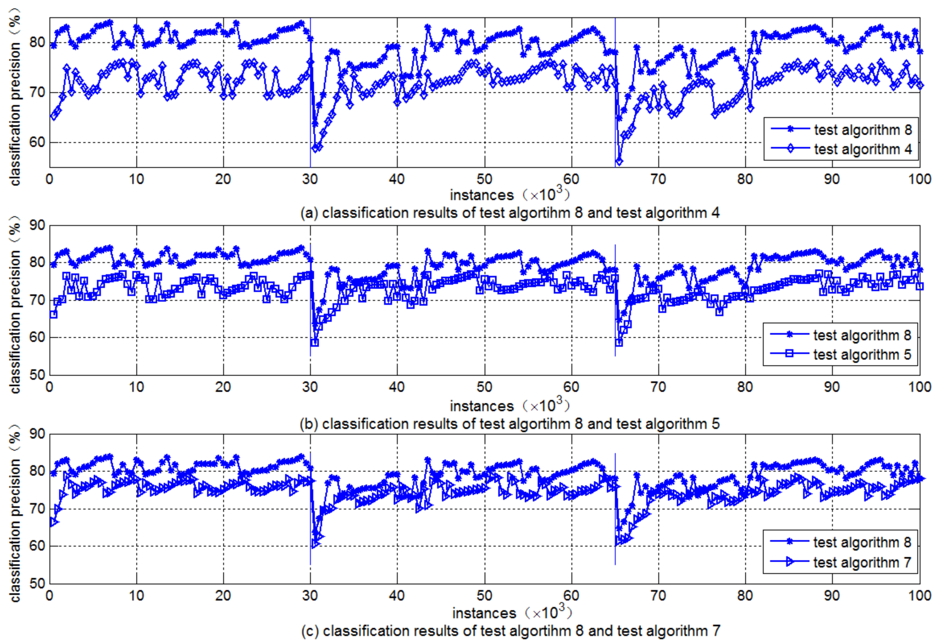
In Figure 2, two sudden concept drifts occurred at 30,000 instances and 65,000 instances (shown as vertical lines). As shown in Figure 2, the classification precision and sensitivity to sudden concept drift of test algorithm 4 are lower than those of test algorithm 5. Test algorithm 8 has a quicker response time to sudden concept drift than the other two test algorithms because it adopts the attribute reduction method and the variable sliding window method based on double thresholds. The higher classification precision also indicates the effectiveness of test algorithm 8. Since the classification precision of test algorithm 4 is the lowest one, subsequent experiments were performed using test algorithms 5, 7, and 8. The average classification precisions of the three test algorithms on the Covertype dataset are shown in

Table 3. Average classification precisions of the three algorithms on the CoverType dataset (%).

Dataset	8	5	7
CoverType	91.33	87.14	88.86

and these experimental results also demonstrate the effectiveness of test algorithm 8.

6.2.2. Memory Use Evaluation

The average memory use of test algorithms 5, 7, and 8 on the three datasets is shown in

Table 4. Average memory use (MB) of the three test algorithms on three datasets.

Dataset	SN of Test Algorithm
	8	5	7
HyperPlane	2.09	4.02	2.97
WaveForm	3.54	5.71	4.26
CoverType	4.21	6.13	5.14

.

As Table 4 shows, in terms of average memory use, test algorithm 8 performs better than the other two test algorithms. In test algorithm 5, the memory use is increased because each new data chunk is used to update the base classifiers. Test algorithm 7 reduces the attributes by comparing the classification error rate of each attribute, which makes its average memory use greater than that of test algorithm 8. The advantage of test algorithm 8 with respect to average memory use shows the effectiveness of the attribute reduction algorithm and the variable sliding window control strategy. For the WaveForm dataset, the attribute reduction results of test algorithm 8 are shown in

Table 5. The number of reduced attributes on the WaveForm dataset.

Instance	Number of Reduced Attributes (The Unit of Sample Interval Is 200)
	1	2	3	4	5	6	7	8
1–1600	22	24	21	23	21	22	21	22
30,000–31,600	24	22	23	22	21	21	22	22
65,000–66,600	23	23	22	22	21	21	21	22

.

In Table 5, the data points indicate the number of reduced attributes of every base classifier. Every $w_b=200$ data points generate a base classifier and there are $L=8$ base classifiers in all. Attribute reduction was performed for every base classifier to maximize the difference between them. The data values in the first row indicate the initial number of reduced attributes of every base classifier when data have just arrived and the data in the other two rows indicate the updating of reduced attributes when the new base classifiers are regenerated because of concept drift. As shown in Table 5, the number of reduced attributes may be slightly larger than the relevant 21 attributes, but the error is less than 3 attributes. The core data attributes are saved and the amount of data is reduced in test algorithm 8.

6.2.3. Time Efficiency Evaluation

The runtimes of test algorithms 5, 7, and 8 on the three datasets are shown in

Table 6. Runtimes (s) of the three test algorithms on three datasets.

Dataset	SN of Test Algorithm
	8	5	7
HyperPlane	23.21	51.22	39.56
WaveForm	46.34	173.65	106.74
CoverType	83.16	334.79	276.38

.

The data in Table 6 shows that the runtime of test algorithm 8 is much less than that of the other two test algorithms. The runtime of test algorithm 5 is highest because of its updating strategy among the base classifiers and lack of attribute reduction. Although test algorithm 7 uses the attribute reduction method by comparing the classification error rate of each attribute, its runtime is still less than that of test algorithm 5, which fully demonstrates the effectiveness of the attribute reduction method in improving the time efficiency of large data processing.

7. Conclusions

To deal with the problem of noise and concept drift in data streams, the base classifier weight updating method and the double-threshold concept drift detection method were introduced in this paper to improve the classification precision of noisy data streams. By controlling the sliding window size in three stages (slow start, drift monitoring, and fast recovery), the detection efficiency of both gradual and sudden concept drift is improved. The approximate attribute reduction algorithm further reduces the resource use and the influence of noise and redundant data in the ensemble classification algorithm. The experimental results on synthetic and real data verify three aspects of the effectiveness among the ensemble classification algorithm including classification precision, memory use, and large gains in runtime. Our ongoing work is to decrease the result error of the attribute reduction algorithm and improve the ensemble classification performance by evaluating the performance of each of the base classifiers further.

References

- Wen, Y.M.; Qiang, B.H.; Fan, Z.G. A survey of the classification of data streams with concept drift. CAAI Trans. Intell. Syst. 2012, 7, 492–501. [Google Scholar] [CrossRef]
- Abbaszadeh, O.; Amiri, A.; Khanteymoori, A.R. An ensemble method for data stream classification in the presence of concept drift. Front. Inf. Technol. Electron. Eng. 2015, 16, 1059–1068. [Google Scholar] [CrossRef]
- Wang, H.X.; FAN, W.; Yu, P.S.; Han, J.W. Mining concept-drifting data streams using ensembles classifiers. In Proceedings of the 9th ACM SIGKDD International Conference on Knowledge Discovery and Data Mining, Washington, DC, USA, 24–27 August 2003; pp. 226–235. [Google Scholar]
- Street, W.N.; Kim, Y.S. A streaming ensemble algorithm (SEA) for large-scale classification. In Proceedings of the 7th ACM SIGKDD International Conference on Knowledge Discovery and Data Mining, San Francisco, CA, USA, 26–29 August 2001; pp. 377–382. [Google Scholar]
- Brzezinsk, D.; Stefanowski, J. Reacting to different types of concept drift: The accuracy updated ensemble algorithm. IEEE Trans. Neural Netw. Learn. Syst. 2014, 25, 81–94. [Google Scholar] [CrossRef]
- Chen, X.D.; Sun, L.J.; Han, C.; Guo, J. Detecting Concept Drift of Data Stream Based on Fuzzy Clustering. Comput. Sci. 2016, 43, 219–223. [Google Scholar] [CrossRef]
- Wang, Z.X.; Sun, G.; Wang, H. Ensemble Classification Algorithm for Data Streams with Noise and Concept Drifts. J. Chin. Comput. Syst. 2016, 37, 1445–1449. Available online: http://xwxt.sict.ac.cn/EN/abstract/abstract3485.shtml (accessed on 20 March 2018).
- Xie, Y.J.; Miao, Y.Q.; Shao, Q.W.; Gao, H.; Wen, Y.M. A Classification Algorithm for Novel Class Detection Based on Data Stream with Concept-drift. J. Guilin Univ. Electron. Technol. 2015, 35, 459–465. [Google Scholar] [CrossRef]
- Gama, J.; Gastillo, G. Learning with Local Drift Detection. In Proceedings of the International Conference on Advanced Data Mining and Applications, Xi’an, China, 14–16 August 2006; pp. 42–55. [Google Scholar]
- Xu, S.L.; Wang, J.H. Classification Algorithm Combined with Unsupervised Learning for Data Stream. Pattern Recognit. Artif. Intell. 2016, 29, 665–672. [Google Scholar] [CrossRef]
- Jiang, F.; Zhang, Y.Q.; Du, J.W.; Liu, G.Z.; Sui, Y.F. Approximate reducts-based ensemble learning algorithm and its application in intrusion detection. J. Beijing Univ. Technol. 2016, 42, 877–885. [Google Scholar] [CrossRef]
- Chen, X.; Wang, X.M.; Huang, Y.; Wang, X.Y. Fault diagnosis for tilt-rotor aircraft flight control system based on variable precision rough set-OMELM. Control Decis. 2015, 30, 433–440. [Google Scholar] [CrossRef]
- Lin, P.R.; Lin, Y.J. Ensemble learning based on model weight and random subspace in noise data. J. Hefei Univ. Technol. 2015, 38, 186–190. [Google Scholar] [CrossRef]
- Jiang, F.; Zhang, Y.Q.; Du, J.W.; Liu, G.Z.; Feng, Y.X. An ensemble learning algorithm based on sampling and reduction. J. Qingdao Univ. Sci. Technol. 2016, 37, 451–464. [Google Scholar] [CrossRef]
- Kuncheva, L.I. Classifier ensembles for changing environments. In Proceedings of the International Workshop on Multiple Classifier Systems, Cagliari, Italy, 9–11 June 2004; pp. 1–15. [Google Scholar] [CrossRef]
- Jacobson, V.; Karels, M.J. Congestion Avoidance and Control. IEEE/ACM Trans. Netw. 1988, 18, 314–329. [Google Scholar] [CrossRef]
- Buhlmann, P.; Yu, B. Analyzing bagging. Ann. Stat. 2002, 30, 927–961. [Google Scholar] [CrossRef]
- Bifet, A.; Holmes, G.; Kirkby, R.; Pfahringer, B. MOA: Massive online analysis. J. Mach. Learn. Res. 2010, 11, 1601–1604. Available online: https://moa.cms.waikato.ac.nz/ (accessed on 20 March 2018).
- UCI Machine Learning Repository. Available online: http://archive.ics.uci.edu/ml (accessed on 20 March 2018).
Figure 1.
Classification precision of the five algorithms on the HyperPlane dataset.
Figure 2.
Classification precision of the four algorithms on the WaveForm dataset.