A Unified Gas Kinetic Scheme for Transport and Collision Effects in Plasma

Abstract

In this study, the Boltzmann equation with electric acceleration term is discretized and solved by the unified gas-kinetic scheme (UGKS). The charged particle transport driven by electric field is included in the electric acceleration term. To capture non-equilibrium distribution function, the probability distribution functions of gas is discretized in a discrete velocity space. After discretization, the numerical flux for distribution function is computed to update the microscopic and macroscopic states. The flux is decided by an integral solution of Boltzmann equation based on characteristic problem. An electron-ion collision model is introduced in the Boltzmann Bhatnagar-Gross-Krook (BGK) equation. This finite volume method for the UGKS couples the free transport and long-range interaction between particles. For simplicity, the electric field induced by charged particles is controlled by the Poisson’s equation, which is solved using the Green’s function for two dimensional plasma system subjected to the symmetry or periodic boundary conditions. Two numerical cases, linear Landau damping and Gaussian beam, are carried out to validate the proposed method. The linear electron plasma wave damping is simulated based on electron-ion collision operator. Comparison results show good accuracy and higher efficiency than particle based methods. Difference between Poisson’s equation and complete electromagnetic Maxwell equation is presented by numerical results based on the two models. Highly non-equilibrium and rarefied plasma flows, such as electron flows driven by electromagnetic field, can be simulated easily. The UGKS-Poisson model is proved to be promising in plasma flow simulation.

1. Introduction

The Boltzmann equation describes time evolution of physical state under external field using gas-distribution function [1]. In description of plasma with long-range Coulomb interaction, Vlasov showed the difficulties when kinetic theory based on standard transport-collision is applied: (1) Theory of pair collisions disagrees with the discovery by Rayleigh, I. Langmuir and L. Tonks that vibrations exist in electron plasma; (2) Theory of pair collisions without Coulomb interaction will lead to divergence of kinetic term; (3) Theory of pair collisions cannot explain results of experiments by H. Merrill and H. Webb that electrons scatter anomalously in gaseous plasma [2]. In gas, binary interaction is taken as the rule. However, in plasma, waves, or organized motion of plasma, are very important because the particles can interact at long ranges through the electric and magnetic forces. Vlasov suggested a source term which contains the Coulomb interaction added in Boltzmann equation. It is a partial differential equation (PDE) for distribution function of particles, which represents probability that particle stays at a specific position and velocity. The acceleration term in the equation describes redistribution of particle on particle phase space due to electromagnetic force.

Many work about numerical methods have been done to model plasma evolution. Particle based method is a direct simulation method by tracing particle trajectory. P. Degond et al. (2010) proposed a particle-in-cell (PIC) method based on Vlasov equation [3]. In PIC method, the particle details, such as the location, velocity, are exactly captured by the equation of motion. To reduce computational cost, finite element method (FEM) and spectral method are proposed. In FEM the whole computational domain is divided into several discrete elements and a polynomial is applied to approximate the distribution function in phase space. N. Crouseilles et al. (2011) proposed a Galerkin method for the Vlasov equation. Lagrange polynomials are applied to construct basis function [4]. D. C. Seal (2012) reported a work in his doctorate thesis that focuses on a discontinuous Galerkin method for the solution of the Vlasov equation. In finite element space, the basis functions used for representation of the distribution function in the Vlasov equation are allowed to be discontinuous at the cell interface [5]. R. Heath et al. (2012) applied penalty function in approximation of discrete distribution function. The rate of convergence is greatly improved [6]. For better accuracy in modelling non-equilibrium distribution function, many researchers constructed spectral methods to solve plasma Vlasov equation. J. W. Schumer et al. (1998) used the Fourier-Hermite polynomial to construct basis functions. Fourth order Runge-Kutta method (RK) is chosen to improve the convergence rate [7]. S. Le Bourdiec et al. (2006) constructed a spectral method based on generalized Hermite functions [8]. N. Crouseilles et al. (2009) proposed a forward semi-Lagrangian spectral method with B-splines basis. Different from previous method, numerical time step can be much larger than particle collision time [9].

Since it is hard to control the truncation error in approximation of gas distribution function, conservative methods based on Godunov’s scheme are proposed [10]. E. Sonnendrücker (1999) et al. first introduced a semi-Lagrangian conservative method [11]. F. Filbet et al. (2001) constructed a particle based conservative method [12]. Since the accuracy of methods is severely influenced by the phase and amplitude error because of dissipation from the way of reconstruction and the use of slope corrector, N. Crouseilles et al. (2007) constructed a conservative method using the Hermite spline interpolation [13]. J. W. Banks et al. (2011) proposed a finite volume method (FVM) to solve the Vlasov equation, in which the PDE is integrated in discrete phase space and the numerical flux of the distribution function through a cell interface is evaluated using high-order approximations of the cell-face average [14]. S. Xu et al. (2015) simulated the Navier-Stokes dielectric barrier discharge (NS-DBD) plasma formation between parallel electrodes in ${\mathrm{N}}_2$-${\mathrm{O}}_2$ mixture air at low-pressure under nanosecond impulses [15]. However, in these schemes, individual particle motion is resolved in flux evaluation so numerical time step is limited within relaxation time.

In current paper, a unified gas kinetic scheme (UGKS) is applied to simulate plasma flows based on the Boltzmann-Poisson equation. The UGKS is proposed by Xu, Huang and Yu [16,17], which attracts more and more researchers’ attention [18,19,20,21,22,23,24,25,26,27,28,29,30,31,32]. In plasma flow, particle transport is controlled by electric force, so the state of gas is decided by electric field. In mathematics, electric force term does not appear in advection part but a source term in discretization. Gas distribution function can never evolve towards Maxwellian as the Bhatnagar-Gross-Krook (BGK) model describes. The real gas distribution function in the highly non-equilibrium region is never able to be described by a Maxwellian. In this paper, the particle velocity space is discretized so that distribution can be exactly described in all flow regimes [16]. The flux reconstruction at the cell interface is treated as the Riemann problem along characteristic curves presented as particle transport velocity [33]. The free transport and interaction between particles are coupled so that the dissipation in the transport process is controlled by the source of the long-range interaction rather than numerical time step. With this technique, the artificial dissipation as the one in J. Banks et al. (2011) [14] will not be brought in numerical process.

With integral solution of Boltzmann equation, The UGKS obtains accurate gas distribution function at cell interface at each time step [33]. The numerical time step can be decided by the Courant-Friedrichs-Lewy (CFL) condition [34]. This high fidelity and efficiency in numerical simulation make the UGKS a better way to solve plasma problems. Based on the BGK model equation, C. liu et al. (2017) simulated multi-scale and multi-component plasma transport based on the UGKS [35]. Many challenging cases including magnetic reconnection problem in the transition regime are simulated. In study of plasma, UGKS provides a reliable multi-scale approach for numerical simulation. In solving the Boltzmann equation, gas distribution function at cell interface is obtained by the solution for the local Riemann problem [10] by using difference biased in the direction determined by the sign of the characteristic speeds [36], thus UGKS has good conservation property and good robustness. Spectral methods has a high order accuracy in smooth regime [37]. However, highly non-equilibrium state will be a challenge because a large error appears in a strong discontinuity at cell interface of phase space. This problem becomes severe when micro-electromechanical systems should also be paid enough attention in rarefied regime [38]. In plasma, time-varying electric field causes collective behavior with many degrees of variation [39,40]. Since the flux of gas distribution function for particles in discrete microscopic velocity space is computed in UGKS, the multi-scale property is satisfied. Therefore, the present UGKS is a promising scheme for plasma simulation.

Unlike neutral gas, plasma consists of a significant number of charge carriers, which makes it electrically conductive. Because of this feature, plasma responds strongly to electromagnetic field. Plasma does not have certain shape or certain volume if not enclosed in a container, but its motion and state are able to be controlled by electromagnetic force. Under influence of electromagnetic field, plasma can be formed into various structures. An important property used to describe the electric field is electric potential. It represents the amount of electrical energy of a unitary point charge at any point in an electric field. The electric potential, which denotes the ability of non static electricity to carrying a charge from reference point to present location, is related to the force directly. The electric potential of a point charge declines as it is driven by an electric force and moving in the direction of electric field line. By Faraday’s law, the electric field has zero curl. Therefore, the electric field can be obtained directly by electric potential. The Maxwell equations are a set of PDEs that describe how the fields vary in space due to sources. In this paper, we concentrate on plasma evolution under electric field so only Poisson’s equation is solved. All cases are tested in symmetric configuration. Green’s function is an efficient approach to solve Poisson’s equation under this condition. In mathematics, an electric field leaving a volume is proportional to the charge inside. The Green’s function is applied to solve the Poisson’s equation which denotes electric potential. Electric potential obtained by the Poisson’s equation is a sum of series whose basis functions are Green’s functions. The basis functions represent Coulomb interaction potential induced by charges in the whole computational domain [41]. After the electric potential is obtained, the electric field can be obtained by spatial gradient of the electric potential. The acceleration term in the Boltzmann equation can be decided. In more generalized cases, UGKS is also able to simulate plasma flows under a correct acceleration term.

The rest of the paper is organized as follows. First, we emphasize the numerical method for solution of the Boltzmann-Poisson equation in Section 2. Then, the Landau damping, Gaussian beam and linear electron plasma wave damping are numerically simulated and the numerical results are presented in Section 3. Finally, some remarks concluded from this study are grouped in Section 4.

2. Numerical Methods

The Boltzmann BGK equation is used for UGKS to simulate plasma. Other collision term can also be adapted to this method via modelling particle relaxation time. The BGK equation can be written as

$$\frac{\partial f}{\partial t}+\mathit{u}\frac{\partial f}{\partial \mathit{x}}+\mathit{a}\frac{\partial f}{\partial \mathit{u}}=\frac{g-f}{\tau },$$

(1)

where f is the particle distribution function of the space $\mathit{x}$, time t, particle velocity $\mathit{u}=(u,v)$, collision time $\tau$, and acceleration $\mathit{a}$ due to electromagnetic field. g is the equilibrium distribution function,

$$g=\rho {\left(\frac{\lambda }{\pi }\right)}^{\frac{K+D}{2}}{e}^{-\lambda \left[{\left(\mathit{u}-\mathit{U}\right)}^2+{\xi }^2\right]},$$

(2)

where K denotes internal freedom degree and D denotes dimension, $\xi$ is the internal freedom of gas, $\mathit{U}$ is the macro velocity and $\rho$ is the density of plasma. In this paper, only two dimensional cases are considered, so the relation between the macroscopic variables $\mathit{W}$ with the microscopic variables $\mathit{\psi }$ is

$$\mathit{W}=\left(\begin{array}{c}\rho \\ \rho U\\ \rho V\\ \rho E\end{array}\right)=\int \mathit{\psi }fdudvd\xi ,$$

(3)

where $\rho E=\frac{1}{2}\rho \left(U^2+V^2+\frac{K+2}{2\lambda }\right)$, and $\mathit{\psi }={(1,u,v,1/2(u^2+v^2+{\xi }^2))}^T$. The pressure and density can be related with $\lambda$ as $p=\rho /2\lambda$.

In discrete particle velocity space, Equation (3) can be written as

$$\mathit{W}=\sum \sum \sum \mathit{\psi }f\Delta u\Delta v\Delta \xi .$$

(4)

where $\Delta u$, $\Delta v$ and $\Delta \xi$ are microscopic velocity intervals. In this discrete integration, the limit is decided by three times of initial Maxwell variance $\left[-3\sigma ,3\sigma \right]$.

In the unified gas kinetic scheme, at the cell interface the solution $f_{cf}$ for Boltzmann BGK equation is constructed from an integral solution using the method of characteristics

$$f_{j,k}\left({\mathit{x}}_{cf},\mathit{u},t\right)=\frac{1}{\tau }{\int }_0^{t}g\left({\mathit{x}}^{\prime },{\mathit{u}}^{\prime },t\right)e^{-\left(t-t^{\prime }\right)/\tau }d{t}^{\prime }+e^{-t/\tau }{\tilde{f}}_{j,k}\left({\mathit{x}}_{cf}-\mathit{u}t,\mathit{u}-\mathit{a}t,0\right).$$

(5)

Here ${\mathit{x}}^{\prime }={\mathit{x}}_{cf}-\mathit{u}t+\frac{1}{2}\mathit{a}{t}^2$ and ${\mathit{u}}^{\prime }=\mathit{u}-\mathit{a}t$ are particle trajectory and velocity, respectively. $\tilde{f}$ is the initial distribution function. Subscript $cf$ denotes cell interface, j and k represent the index of particle velocities u, v. Inside each control volume of physical space and discrete particle velocity space, the gas distribution function at the beginning of time step is computed using a linear reconstruction [17]

$${\tilde{f}}_{j,k}\left({\mathit{x}}_{cf}-\mathit{u}t,\mathit{u}-\mathit{a}t,0\right)=\left\{\begin{array}{ll}{f}_{cf,j,k}^l-{\left(\frac{\partial f}{\partial \mathit{x}}\right)}_{cf,j,k}^l·\mathit{u}t-{\left(\frac{\partial f}{\partial \mathit{u}}\right)}_{cf,j,k}^l\mathit{a}t,& \mathit{u}·{\mathit{S}}_{cf}\ge 0,\\ f_{cf,j,k}^r-{\left(\frac{\partial f}{\partial \mathit{x}}\right)}_{cf,j,k}^r·\mathit{u}t-{\left(\frac{\partial f}{\partial \mathit{u}}\right)}_{cf,j,k}^r\mathit{a}t,& \mathit{u}·{\mathit{S}}_{cf}<0,\end{array}\right.$$

(6)

where l and r represent left and right of cell interface. In a two dimensional configuration, i represents cell index of an unstructured mesh. Under unstructured mesh, spatial derivatives of distribution functions can be obtained via least square method. The approximation of the partial derivative of f with respect to the particle velocity $\mathit{u}$ can be written as

$$\begin{array}{c}{\left(\frac{\partial f}{\partial u}\right)}_i=\frac{f_{i,j+1,k}-f_{i,j-1,k}}{2\Delta u},\\ {\left(\frac{\partial f}{\partial v}\right)}_i=\frac{f_{i,j,k+1}-f_{i,j,k-1}}{2\Delta v}.\end{array}$$

(7)

For a second order scheme, it is an appropriate approach. An efficient fast spectral method can also be implemented in UGKS solver for high order accuracy [42]. At the boundary of particle velocity space for two dimensional plasma, distribution function is set to be zero.

For integral term of equilibrium distribution function in Equation (5), continuous particle velocity space is applied to evaluate this Maxwell distribution function. Around cell interface $cf$, it can be expanded as

$$g\left({\mathit{x}}^{\prime },{\mathit{u}}^{\prime },t\right)=\left\{\begin{array}{ll}{g}_0\left(\mathit{x},\mathit{u},0\right)\left[1-\left(t-t^{\prime }\right){\overline{\mathit{a}}}^l·\mathit{u}-\left(t-t^{\prime }\right){\overline{\mathit{b}}}^l·\mathit{a}+\overline{A}{t}^{\prime }\right],& \mathit{u}·{\mathit{S}}_{cf}\ge 0,\\ g_0\left(\mathit{x},\mathit{u},0\right)\left[1-\left(t-t^{\prime }\right){\overline{\mathit{a}}}^r·\mathit{u}-\left(t-t^{\prime }\right){\overline{\mathit{b}}}^r·\mathit{a}+\overline{A}{t}^{\prime }\right],& \mathit{u}·{\mathit{S}}_{cf}<0,\end{array}\right.$$

(8)

where $g_0(\mathit{x},\mathit{u},0)$ is local Maxwellian located at cell interface which reads

$$g_0\left(\mathit{x},\mathit{u},0\right)={\rho }_0{\left(\frac{{\lambda }_0}{\pi }\right)}^{\frac{K+D}{2}}{e}^{-{\lambda }_0\left[{\left(\mathit{u}-{\mathit{U}}_0\right)}^2+{\xi }^2\right]},$$

(9)

where $\overline{\mathit{a}}$ and $\overline{A}$ are derivatives of Maxwellian in space and time. They can be obtained from Taylor expansion of Maxwellian. $\overline{\mathit{b}}$ is the derivative term of Maxwellian g with respect to the particle velocity $\mathit{u}$. In a two dimensional configuration, they have the following form,

$$\begin{array}{ccc}\hfill {\overline{a}}_n& =& {\overline{a}}_{{}_n}^1+{\overline{a}}_{{}_n}^{2}u+{\overline{a}}_{{}_n}^{3}v+{\overline{a}}_{{}_n}^4\frac{1}{2}\left(u^2+v^2+{\xi }^2\right),\hfill \\ \hfill {\overline{a}}_t& =& {\overline{a}}_{{}_t}^1+{\overline{a}}_{{}_t}^{2}u+{\overline{a}}_{{}_t}^{3}v+{\overline{a}}_{{}_t}^4\frac{1}{2}\left(u^2+v^2+{\xi }^2\right),\hfill \\ \hfill {\overline{A}}_n& =& {\overline{A}}_{{}_n}^1+{\overline{A}}_{{}_n}^{2}u+{\overline{A}}_{{}_n}^{3}v+{\overline{A}}_{{}_n}^4\frac{1}{2}\left(u^2+v^2+{\xi }^2\right),\hfill \end{array}$$

(10)

where n and t represent the normal and tangential direction component respectively. Macroscopic variables in Equation (9) are determined by the compatibility condition of BGK model. The conservation constraints are given as

$${\mathit{W}}_0=\int \mathit{\psi }{g}_0\left(\mathit{x},\mathit{u},0\right)d\mathrm{\Xi }=\int \mathit{\psi }\left(g^{l}H\left[u_n\right]+g^r\left(1-H\left[u_n\right]\right)\right)d\mathrm{\Xi },$$

(11)

where H is Heaviside function defined by

$$H\left[x\right]=\left\{\begin{array}{ll}0,& x<0,\\ 1,& x\ge 0.\end{array}\right.$$

(12)

The normal derivatives term can be obtained by the relation between the spatial derivatives of the distribution function and the conservation variables,

$$\begin{array}{ccc}\hfill \frac{{\mathit{W}}_0-{\mathit{W}}^l}{{\rho }_0\Delta x^l}& =& \int {\overline{a}}_n^l\mathit{\psi }{g}_0\left(\mathit{x},\mathit{u},0\right)d\mathrm{\Xi },\hfill \\ \hfill \frac{{\mathit{W}}^r-{\mathit{W}}_0}{{\rho }_0\Delta x^r}& =& \int {\overline{a}}_n^r\mathit{\psi }{g}_0\left(\mathit{x},\mathit{u},0\right)d\mathrm{\Xi }.\hfill \end{array}$$

(13)

For the two dimensional problems, the the normal and tangential component of $\overline{\mathit{b}}$ in Equation (8) read

$$\begin{array}{c}\hfill g_0\left(\mathit{x},\mathit{u},0\right){\overline{b}}_n=\frac{\partial g\left(\mathit{x},\mathit{u},0\right)}{\partial u}=-2\lambda \left(u-U\right)g_0\left(\mathit{x},\mathit{u},0\right),\\ \hfill g_0\left(\mathit{x},\mathit{u},0\right){\overline{b}}_t=\frac{\partial g\left(\mathit{x},\mathit{u},0\right)}{\partial v}=-2\lambda \left(v-V\right)g_0\left(\mathit{x},\mathit{u},0\right).\end{array}$$

(14)

Now, we have determined all parameters of the initial distribution function and the Maxwell distribution function in Equation (5). After substituting these parameters into the formula of gas distribution function, we have

$$\begin{array}{cc}\hfill f_{j,k}\left({\mathit{x}}_{cf},\mathit{u},t\right)=& \left(1-e^{-\frac{t}{\tau }}\right)g\left({\mathit{x}}^{\prime },{\mathit{u}}^{\prime },t\right)+\left(e^{-\frac{t}{\tau }}\left(t+\tau \right)-\tau \right)\left({\overline{a}}_n^l\mathit{u}·\mathit{n}+{\overline{b}}_n^l{a}_n\right)H\left[\mathit{u}·\mathit{n}\right]g\left({\mathit{x}}^{\prime },{\mathit{u}}^{\prime },t\right)\hfill \\ & +\left(e^{-\frac{t}{\tau }}\left(t+\tau \right)-\tau \right)\left({\overline{a}}_n^r\mathit{u}·\mathit{n}+{\overline{b}}_n^r{a}_n\right)\left(1-H\left[\mathit{u}·\mathit{n}\right]\right)g\left({\mathit{x}}^{\prime },{\mathit{u}}^{\prime },t\right)\hfill \\ & +\left(e^{-\frac{t}{\tau }}\left(t+\tau \right)-\tau \right)\left({\overline{a}}_{t}v+{\overline{b}}_t{a}_t\right)g\left({\mathit{x}}^{\prime },{\mathit{u}}^{\prime },t\right)\hfill \\ & +\left[t-\tau \left(1-e^{-\frac{t}{\tau }}\right)\right]\overline{A}g\left({\mathit{x}}^{\prime },{\mathit{u}}^{\prime },t\right)\hfill \\ & +e^{-\frac{t}{\tau }}\left(\left(f_{0,j,k}^l-{\left(\frac{\partial f}{\partial \mathit{x}}\right)}_{cf,j,k}^l·\mathit{u}t-{\left(\frac{\partial f}{\partial \mathit{u}}\right)}_{cf,j,k}^l\mathit{a}t\right)H\left[\mathit{u}·\mathit{n}\right]\right)\hfill \\ & +e^{-\frac{t}{\tau }}\left(\left(f_{0,j,k}^r-{\left(\frac{\partial f}{\partial \mathit{x}}\right)}_{cf,j,k}^r·\mathit{u}t-{\left(\frac{\partial f}{\partial \mathit{u}}\right)}_{cf,j,k}^r\mathit{a}t\right)\left(1-H\left[\mathit{u}·\mathit{n}\right]\right)\right),\hfill \end{array}$$

(15)

where $\mathit{n}$ denotes the normal vector of interface.

Finally, the macroscopic variables and discrete gas distribution function are updated respectively. For macroscopic conservative variables, we have

$${\mathit{W}}^{n+1}={\mathit{W}}^n-\frac{1}{\mathsf{\Omega }}\mathit{F}·\mathit{S}+\mathit{Sr},$$

(16)

where $\mathsf{\Omega }$ is volume of a cell and $\mathit{S}$ is the area of all the interfaces of the cell. The flux of macroscopic conservative variables reads

$$\mathit{F}={\int }_0^{\Delta t}\int \mathit{u}·\mathit{n}\mathit{\psi }{f}_{cf}\left(\mathit{x},\mathit{u},t\right)d\mathrm{\Xi }dt.$$

(17)

The source term $\mathit{Sr}$ is induced by inaccurate computation of reconstruction. The acceleration term does not appear in the evaluation of the particle trajectory when solving the gas distribution function at the cell interface. So a source term should be added in the projection stage [43], which reads

$$\mathit{S}r=\left(\begin{array}{c}0\\ \rho a_x\Delta t\\ \rho a_y\Delta t\\ \overrightarrow{F_{\rho }}·\overrightarrow{a}\end{array}\right).$$

(18)

In above equations, integration under particle velocity space takes a discrete form. For discrete gas distribution function in each cell of physical space and particle velocity space, the update is realized by

$$f_{i,j,k}^{n+1}=f_{i,j,k}^n-\frac{1}{\mathsf{\Omega }}{\int }_0^{\Delta t}\mathit{u}·\mathit{S}{f}_{cf}\left(\mathit{x},\mathit{u},t\right)dt+\frac{\Delta t}{2}\left(\frac{g_{i,j,k}^{n+1}-f_{i,j,k}^{n+1}}{{\tau }^{n+1}}+\frac{g_{i,j,k}^n-f_{i,j,k}^n}{{\tau }^n}\right).$$

(19)

In all above formulas, the relaxation time $\tau$ is related to different scales of particles in plasma, which reads [35]

$${\tau }_{\alpha }=\frac{1}{{\displaystyle \sum _{\kappa }}\frac{{\theta }_{\alpha \kappa }{\rho }_{\kappa }}{m_{\kappa }}},$$

(20)

where ${\rho }_{\kappa }$ represents density of component $\kappa$, $m_{\kappa }$ represents particle mass of component $\kappa$ and ${\theta }_{\alpha \kappa }$ represents collision frequency coefficient between component $\alpha$ and $\kappa$,

$${\theta }_{\alpha \kappa }=\frac{4\sqrt{\pi }}{3}\left(\frac{2k_B{T}_{\alpha }}{m_{\alpha }}+\frac{2k_B{T}_{\kappa }}{m_{\kappa }}\right){\left(\frac{d_{\alpha }+d_{\kappa }}{2}\right)}^2,$$

(21)

where T represents temperature, $k_B$ represents Boltzmann constant, and d represents diameter of particle.

Next, we will introduce the process of solving the electromagnetic Poisson’s equation. Solving the Poisson’s equation amounts to finding the electric potential $\mathsf{\Phi }$ for a given charge distribution. The mathematical details behind the Poisson’s equation in electrostatics are described by Gauss’s law for electricity [44]. The Poisson’s equation applied in our work is written as

$$\Delta \mathsf{\Phi }=-\frac{{\rho }_c}{\epsilon },$$

(22)

where ${\rho }_c$ is the charge density and $\epsilon$ is the permittivity of the medium. Equation (22) is solved using the Green’s function [45]. First, we find the particular solution.

$${\mathsf{\Phi }}_i=\frac{1}{\epsilon }\sum _{j=1}^{Nc}G\left({\mathit{x}}_i,{\mathit{x}}_j\right)Q_j,$$

(23)

where $Nc$ represents the number of cells, i represents the cell being studied, j represents cells in discrete computational domain and $j\ne i$. $Q_j$ represents charge in cell j. $G\left({\mathit{x}}_i,{\mathit{x}}_j\right)$ is the Green’s function for the Poisson’s equation, which can be written as

$$G\left({\mathit{x}}_1,{\mathit{x}}_2\right)=\frac{1}{4\pi |{\mathit{x}}_1-{\mathit{x}}_2|}.$$

(24)

In the Green’s function, ${\mathit{x}}_1$ and ${\mathit{x}}_2$ represent radius vectors for two locations of charges. To give a unique Green’s function, symmetry or periodic boundary conditions should be implemented [46]. According to the Faraday’s law, the electric field from charged particles is a conservative vector field. The electric potential $\mathsf{\Phi }$ can be defined [47], such that

$${\mathit{E}}_{self}=-\nabla \mathsf{\Phi }.$$

(25)

Equation (25) is used for the electrostatic part of the electric field. The electrodynamic part of the electric field is induced by magnetic field due to motion of charged particles. If the magnetic field is taken into consideration, the electric field induced by charged particles can be written as

$${\mathit{E}}_{self}=-\nabla \mathsf{\Phi }-\frac{\partial \mathit{A}}{\partial t},$$

(26)

where $\mathit{A}$ is the magnetic vector potential [48]. The relation between the magnetic field $\mathit{B}$ and $\mathit{A}$ can be written as

$$\mathit{B}=\nabla \times \mathit{A}.$$

(27)

The component of particle acceleration due to the electrostatic part of electric field obtained by particular solution via the Green’s function and electrodynamic part of electric field induced by magnetic field is computed as,

$$\mathit{a}=-\frac{q_i}{m}\left(\nabla \mathsf{\Phi }+\frac{\partial \mathit{A}}{\partial t}\right)=-\frac{q_i}{m}\left(\frac{1}{\epsilon }\sum _{j=1}^{Nc}\nabla G\left({\mathit{x}}_i,{\mathit{x}}_j\right)Q_j+\frac{\partial \mathit{A}}{\partial t}\right),$$

(28)

where $q_i$ is the charge of the particle in cell i, m is the mass of the particle. In this paper, the charge to mass ratio of the particle, $\frac{q}{m}$, is a non-dimensional value which satisfies the relation $\left|\frac{q}{m}\right|=1$.

Besides the electric field induced by the charged particles, the external electric field ${\mathit{E}}_{appl}$ also contributes to variation of distribution function. So the acceleration term in Equation (1) includes two parts.

$$\mathit{a}={\mathit{a}}_{self}+{\mathit{a}}_{appl},$$

(29)

After substituting Equations (6), (7) and (29) into Equation (5), we can update the distribution function at $n+1$ step. The above procedure can be repeated in the next time level.

3. Numerical Results

3.1. Linear Landau Damping

The Landau damping is the effect of damping of longitudinal space charge waves in plasma [49]. It prevents an instability from developing and creates a region of stability in the parameter space [50]. Energy exchange between electromagnetic wave in phase space and charged particles in plasma is the cause of Landau damping. In evolution, particles interact strongly with the wave [51]. In current work, we simulate the Landau damping based on the UGKS to study the way in which electrons interact and exchange energy with electromagnetic field. This case is used to test the accuracy of the UGKS for solving the Boltzmann equation in describing time-variant electromagnetism parameters such as electric field and electric potential energy. First, an electromagnetic wave should be added to flow field. This wave is caused by an initial disturbance of distribution function [52].

In current work, 2D initial condition is set to

$$f_0=\rho \frac{\lambda }{\pi }{e}^{-\lambda \left({\left(u-U\right)}^2+{\left(v-V\right)}^2\right)}\left(1+\alpha \cos \left(k_{x}x\right)\cos \left(k_{y}y\right)\right),$$

(30)

where $\lambda =0.5$, $U=V=0$ , $\alpha =0.05$ and the wave numbers $k_x=k_y=0.5$ in current problem. In this case, the scales of non dimensional axis of X and Y are set to be $4\pi$ for a period in disturbance.

In the linear Landau damping case, a periodic boundary condition is applied. The four dimensional phase space contains 64 points per dimension. The particle velocity is truncated at $6.0$. The periodic boundary condition is chosen for 2D linear Landau damping. The length for computational domain in each dimension is set to be $4\pi$. The constant time step $\Delta t$ is chosen as $0.01$. The evolution of density contour is presented in Figure 1. The energy of electric field is being carried away by electrons moving at the phase space. To show this process, the evolution of symmetric electric field and electric energy will be given. First, we computed the average of symmetric electric field. The logarithmic scale of it is used for damping process of electric field, which is presented in Figure 2. In evolution, non dimensional numerical time is decided by $t/t^{*}$. Reference time $t^{*}=L_{r}ef/C$, in which $L_{r}ef=4\pi$ and C denotes speed of sound.

Now, the electric potential energy is computed to show the process of energy transport and conversion during interaction between the electric field and electrons. The electric potential energy is a potential energy that results from coulomb forces between charges. This kind of energy is associated with the configuration of a defined system which contains a certain number of charged particles. In physics, the electric potential energy of a system is the energy required for assembling charges from an infinite distance by bringing them close together. If an object has electric potential energy $U_E$, two key elements are crucial: (1) this object keeps its own charge; (2) it stays at a relative position to other electrically charged objects.

$$U_E=q\mathsf{\Phi }.$$

(31)

The evolution of potential energy in systems with time-variant electric fields is given in Figure 3.

In the current work, we obtain the same evolution process of the electric field and electric energy as Reference [12]. Many works have been done to study the physical picture of Landau damping. Linearized theory is the simplest and rather complete way [53], but it is not physically reasonable because interaction between charged particles and electromagnetic field is coupled with particle transport in the Boltzmann equation. The linearized method is not appropriate to be used in this nonlinear system. However, nonlinearity has been a longstanding problem. To model nonlinear level in the Vlasov equation, a class of exponentially damped solutions of the Vlasov-Poisson equation is proposed [54]. This method fails to explain the mechanism of energy transport although it approximates the damping curves in a mathematical way. The UGKS shows a great advantage on correctly representation for the Landau damping with a much lower computational cost than particle-based methods, which makes it a promising method in plasma simulation.

3.2. Nonlinear Landau Damping

In linear Landau damping case discussed above, the non-equilibrium phenomenon is still not very significant because the initial perturbation of density is very small. In this example, we increase amplitude of the initial perturbation of density in 1D space. The perturbation rate is set to be $\alpha =0.5$. The wave number and periodic length remain the same $k=0.5$ and non dimensional scale of axis $L=4\pi foraperiodindisturbance$. The initial particle distribution function reads:

$$f=\frac{1}{\sqrt{2\pi }}{e}^{-\frac{u^2}{2}}\left(1+\alpha \cos \left(kx\right)\right).$$

(32)

In UGKS, the discrete particle velocity space is applied. The 1D velocity space is truncated at $\left[-6,6\right]$ with 128 intervals. When the velocity space is being discretized, we used cosine to decide the positions of discrete velocity points so that a high resolution can be obtained near the peak of distribution function. This equation is written as

$$u_x=-v_{\max }\left(1+\cos \left(-\frac{\pi }{2}+\pi \frac{i}{Nu-1}\right)\right),$$

(33)

where $v_{\max }$ is the maximum of particle velocity and $Nu$ is the number of discrete velocities of particle. The non dimensional scale of microscopic velocity space is decided by $U/C$, in which C denotes speed of sound.

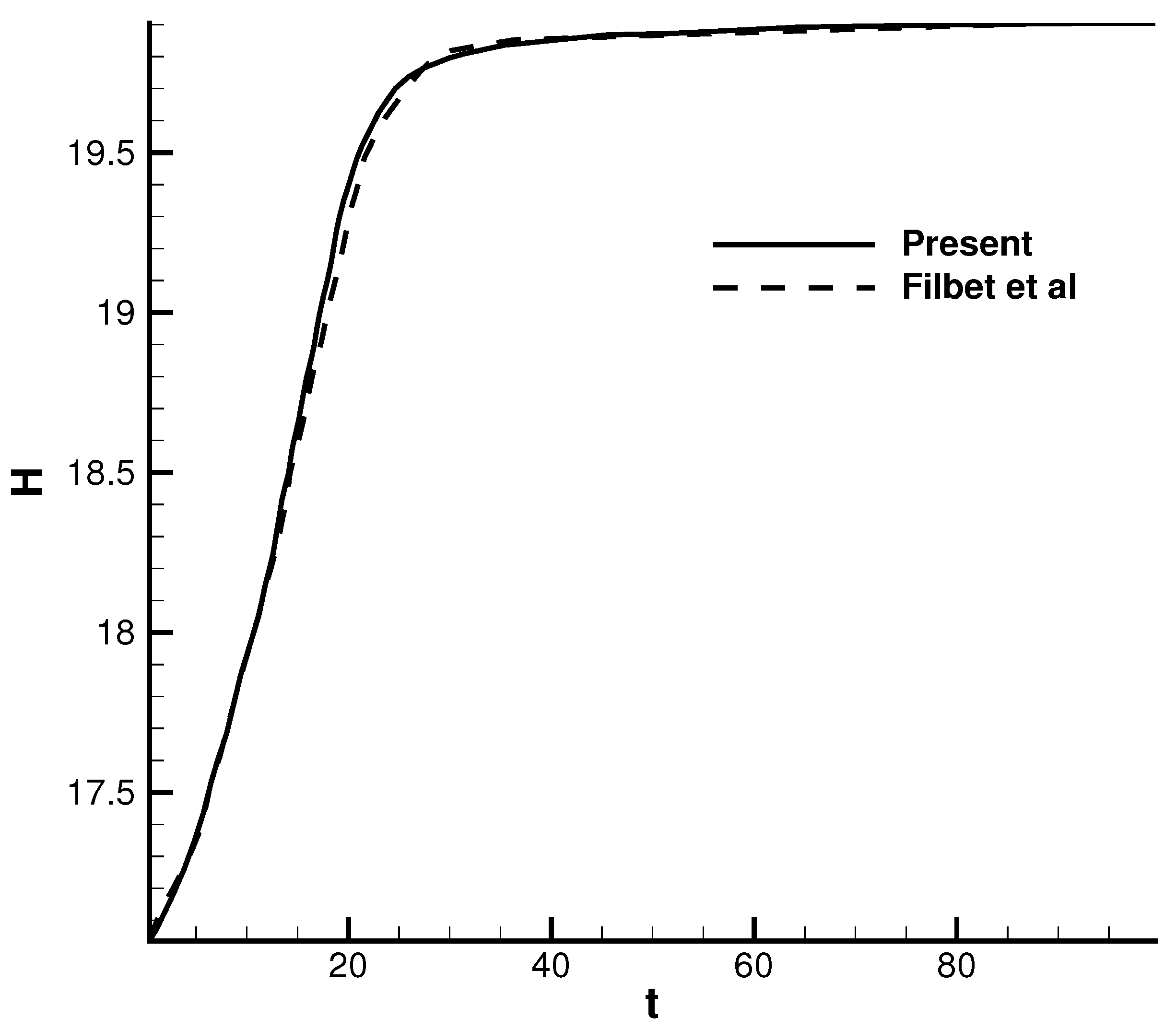
The evolution of the kinetic entropy is taken as a benchmark solution. Traditional FEMs always overestimate this value.The particle-based methods may be an alternative, but computational cost would be overwhelming. The UGKS is able to obtain the same accuracy as particle-based method but calls for much lower computational cost. The comparison result between UGKS and Filbet et al. [12] is presented in Figure 4. The kinetic entropy is computed by $H=-\sum f\ln f$. In evolution, non dimensional numerical time is decided by $t/t^{*}$. Reference time $t^{*}=L_{r}ef/C$, in which $L_{r}ef=4\pi$.

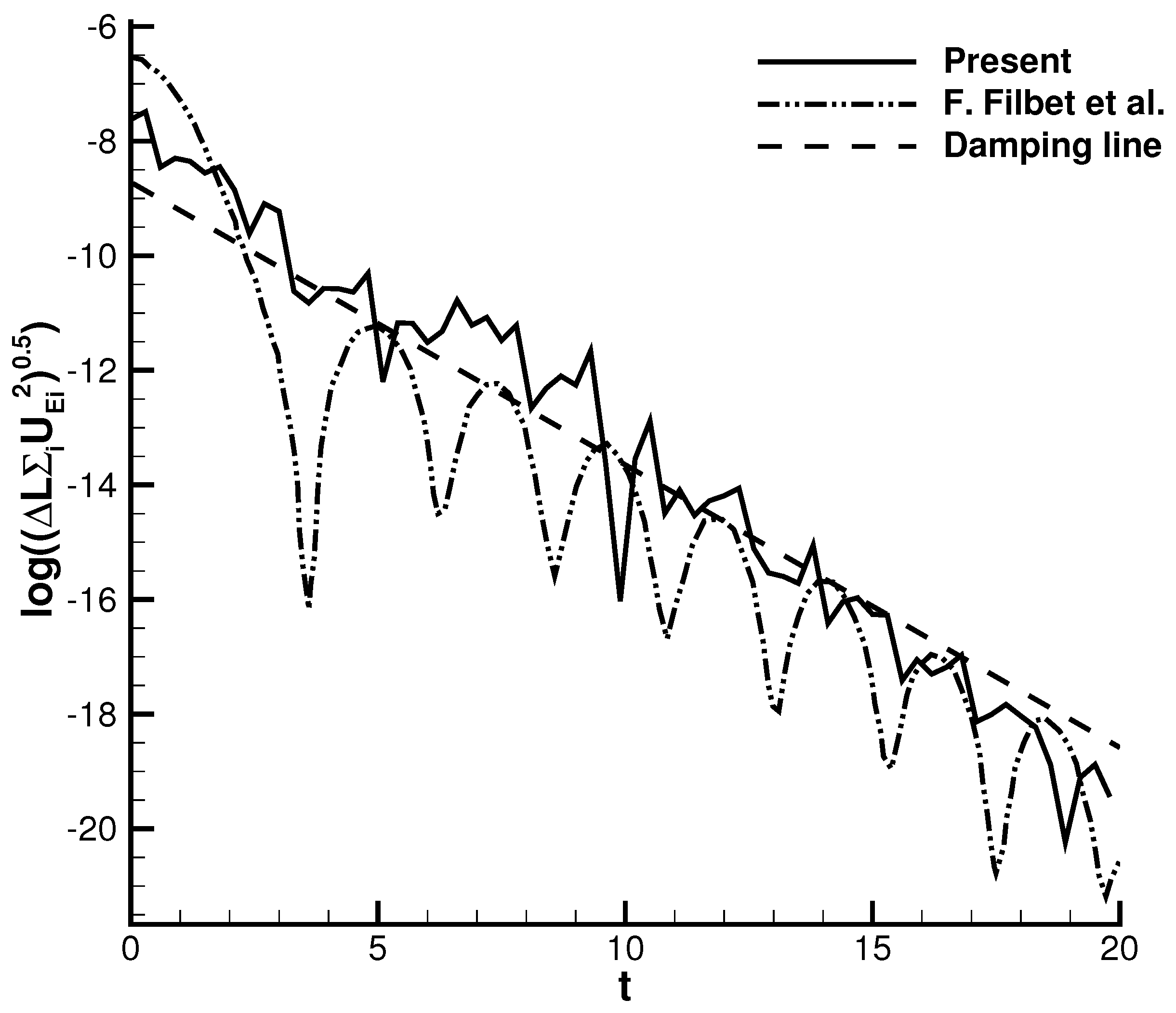
Another benchmark result is $L^2$-norm of the distribution function. Variation of $L^2$-norm is often used to show the rate of negative values because the global mass $\int fd\mathrm{\Xi }$ should be preserved. This value $\sum f^2$ is used to test the characteristics of conservative of UGKS in simulation for plasma flow. The comparison result of $L^2$-norm between UGKS and Filbet et al. [12] is given in Figure 5.

The results of UGKS fit well with the ones of the particle-based method. With a much lower computational cost, the UGKS can archive the same accuracy. The UGKS has a good conservation property and good accuracy in reconstruction, so that the spurious dissipation is avoided. The nonlinear Landau damping case is a highly non-equilibrium phenomenon. To show this, particle distribution functions at different time steps at the center of space are presented in Figure 6.

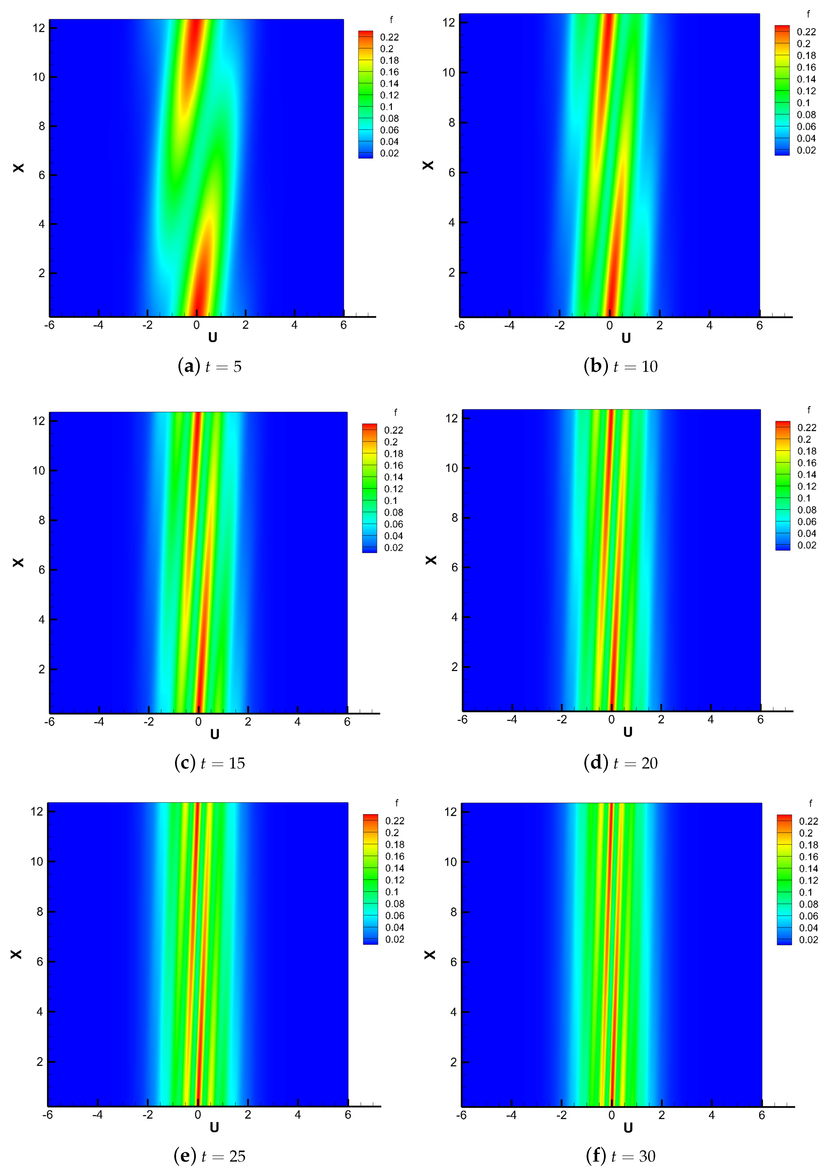
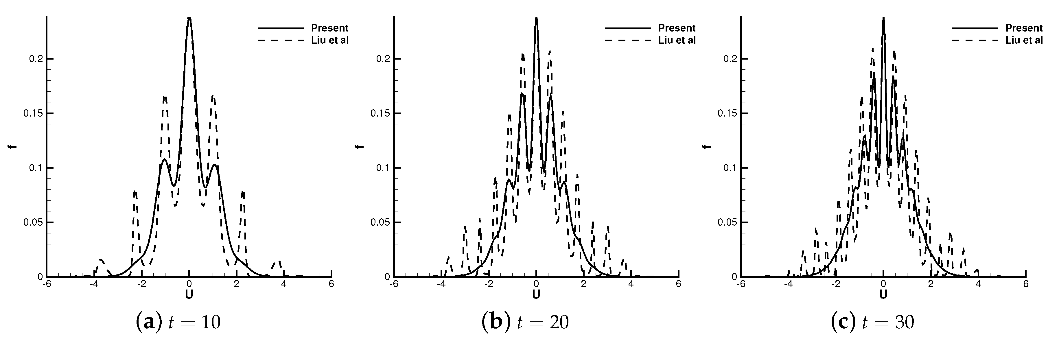
Figure 6 shows the distribution function in velocity space. To give a better description of particle distribution in phase space, the distribution function in the $\left(x,u\right)$ space is presented in Figure 7. Distribution functions at $x=0$ for $t=10,20,30$ are given in Figure 8 to compare with the results in Reference [35]. The heaps of distribution profiles fit with each other. However, difference between Poisson’s equation in this paper and complete Maxwell equation causes inconsistent results. To simplify computation and reduce computational cost, only electric Poisson’s equation is considered. However, in simulation of plasma in electric field, it is an accurate method.

In nonlinear Landau damping case, nonlinear effect dominates the evolution of particle motion and electric field. UGKS successfully captures the unsteady and highly nonlinear waves in plasma. Numerical scheme proposed in this paper provides an accurate method for highly non-equilibrium plasma flow simulation. Time development of entropy under meshes with different cell size $N_x$ and discrete velocity space with different number of points $N_u$ are given in Figure 9. The computation results convergence at $N_x=128$ and $N_u=128$ for present method.

3.3. Gaussian Beam

In the optical field, the Gaussian beam is a beam of monochromatic electromagnetic radiation which has a Gaussian intensity profile. As a result, it has a transverse electromagnetic field given by the Gaussian function. Such a beam can be expanded and focused through lens thus becomes different Gaussian beam at different time steps. According to the theory of quantum mechanics, electrons can both interact with other particles and be diffracted. It has properties of particle and wave [55]. For Gaussian beam case, a beam of electrons is a good model since both interaction between particles due to electromagnetic force and intensity of light should be simulated. In current paper, we choose an electron beam as model to be deformed by the electromagnet field. In addition, the external electric field plays a role of lens. In evolution of beam, the external electric field has an opposite direction to electric field induced by electron itself. In the Boltzmann equation, the acceleration term is from the electric field which includes two parts: Electric field ${\mathit{E}}_{self}$ induced by electron given by the Poisson’s equation and external electric field ${\mathit{E}}_{appl}$. The external electric field is decided by self-consistent field method (SCF) using initial electric field induced by electrons. In current work, the external electric field is linear with respect to spatial coordinates. The relation between ${\mathit{E}}_{self}$ and ${\mathit{E}}_{appl}$ can be written as

$${\mathit{E}}_{self}+{\mathit{E}}_{appl}=-{\omega }^2\mathit{r},$$

(34)

where $\omega$ represents the difference between the initial self-consistent electric field due to particle charges and the linear external electric field. Its value is decided by a self-consistent domain.

$$I=\left\{\left(\overline{x},\overline{y},\overline{u},\overline{v}\right)|\frac{{\overline{x}}^2}{a^2}+\frac{{\overline{y}}^2}{a^2}+\frac{{\overline{u}}^2}{{\left(\omega a\right)}^2}+\frac{{\overline{v}}^2}{{\left(\omega a\right)}^2}=1\right\}.$$

(35)

All values in Equation (35) are nondimensionalized by the root mean square (RMS) thermal velocity $v_{th}$. The RMS results for space and particle velocity are computed by

$$\begin{array}{cc}\hfill \sqrt{{\overline{x}}^2}& =\sqrt{\frac{\int x^{2}fd\mathrm{\Xi }d\mathsf{\Omega }}{\int fd\mathrm{\Xi }d\mathsf{\Omega }}}=a,\sqrt{{\overline{y}}^2}=\sqrt{\frac{\int y^{2}fd\mathrm{\Xi }d\mathsf{\Omega }}{\int fd\mathrm{\Xi }d\mathsf{\Omega }}}=a,\hfill \\ \hfill \sqrt{{\overline{u}}^2}& =\sqrt{\frac{\int u^{2}fd\mathrm{\Xi }d\mathsf{\Omega }}{\int fd\mathrm{\Xi }d\mathsf{\Omega }}}=\omega a,\sqrt{{\overline{v}}^2}=\sqrt{\frac{\int v^{2}fd\mathrm{\Xi }d\mathsf{\Omega }}{\int fd\mathrm{\Xi }d\mathsf{\Omega }}}=\omega a.\hfill \end{array}$$

(36)

For Gaussian beam case, the initial self-consistent electric field is linear in space. So we can obtain the two unknown variables $\omega$ and a using RMS thermal velocity $v_{th}$,

$$a=\frac{r_a}{2},v_{th}=\frac{\omega r_a}{2},$$

(37)

where $r_a$ is the radius of beam. Now we introduce a tune depression factor $\chi =\frac{{\omega }_0}{\omega }$ such that we can adjust external electric field with initial self-consistent electric field. The linear external electric field whose direction is opposite to initial self-consistent electric field can be written as

$${\mathit{E}}_{appl}={\omega }_0^2\mathit{r}.$$

(38)

In the evolution of a beam, the external electric field ${\mathit{E}}_{appl}$ is used to focalize the beam. The dimensionless form of Equation (1) can be rewritten as

$$\frac{\partial f}{\partial t}+\mathit{u}\frac{\partial f}{\partial \mathit{x}}+\left(-\left({\mathit{E}}_{self}+{\mathit{E}}_{app}\right)\right)\frac{\partial f}{\partial \mathit{u}}=\frac{g-f}{\tau }.$$

(39)

The negative sign $“-”$ is because of the negative charge carried by electron.

The 2D initial condition is written as

$$f_0=\left\{\begin{array}{cc}\rho \frac{\lambda }{\pi }{e}^{-\lambda \left({\left(u-U\right)}^2+{\left(v-V\right)}^2\right)}& x^2+y^2\le r_a^2,\\ 0& x^2+y^2>r_a^2.\end{array}\right.$$

(40)

In kinetic theory, $\lambda$ can be obtained by [56]

$$\lambda =\frac{m}{2k_{B}T},$$

(41)

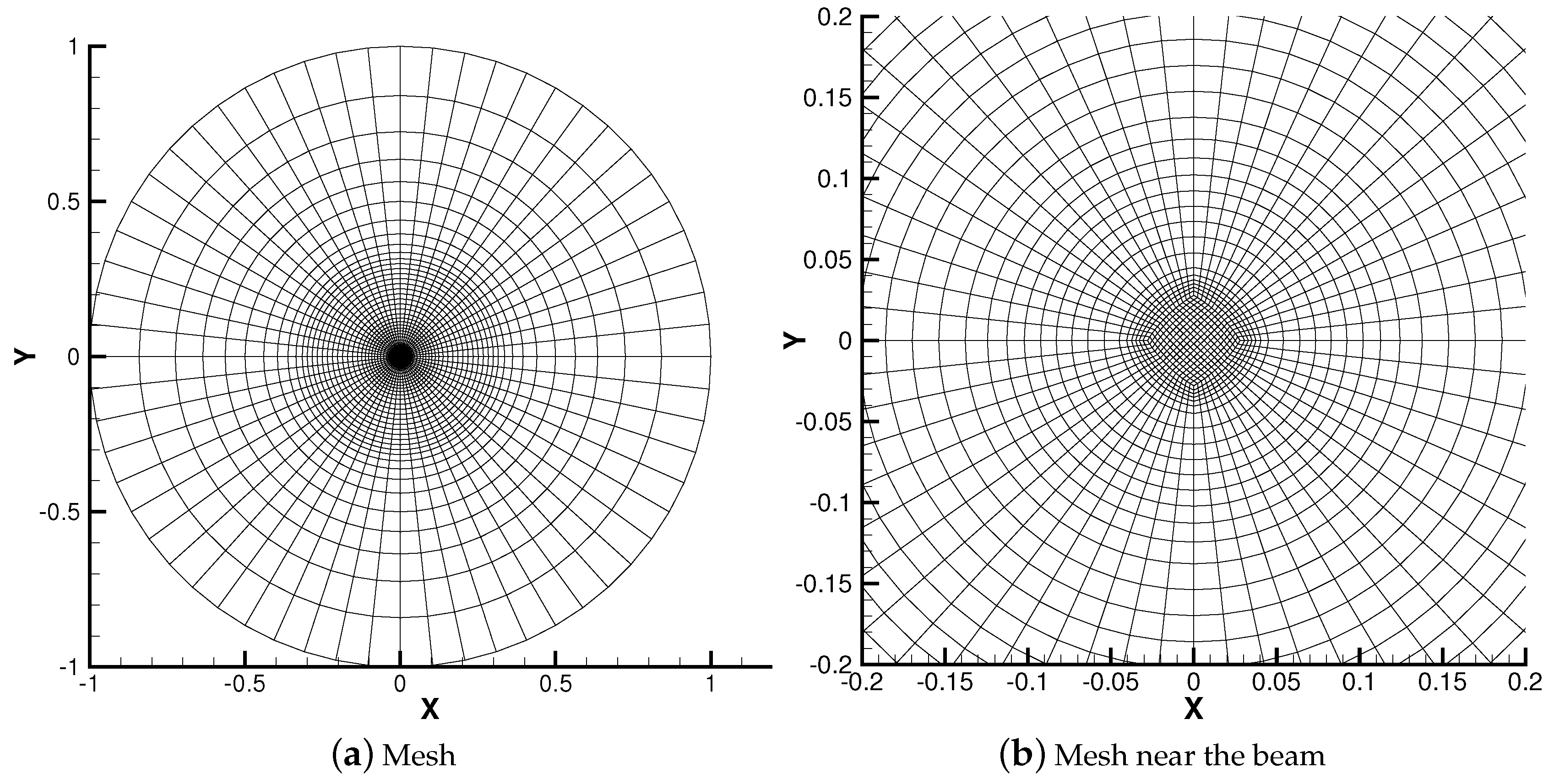
where m is the particle mass, $k_B$ is the Boltzmann constant, T is the temperature. The mesh for beam case has a round boundary, which is shown in Figure 10. In this case, 4032 mesh cells are used to discretize the computational domain.

Absorbing boundary condition (ABC) is applied in Gaussian beam case. The buffer zone is added between the computational domain and boundary with a range ${0.5}^2<x^2+y^2<{1.0}^2$. The flux damps along warp of a circular zone in buffer zone.

$$F_{r_o}=\delta F_{r_i},$$

(42)

where $\delta$ is damping rate, $r_o$ and $r_i$ are the two location on a warp line respectively. The damping rate can be computed as

$$\delta =\cos \left(\frac{\pi }{2}\frac{r-r_i}{r_o-r_i}\right),$$

(43)

where $r_i$ and $r_o$ represent the two limit of buffer zone. In our work, we have

$$\begin{array}{c}{r}_i=0.5,\\ r_o=1.0.\end{array}$$

(44)

The location for $F_{r_o}$ and $F_{r_i}$ is described in Figure 11.

In evolution, the electric field induced by charged particles and particle free transport will expand the beam. Applied external electric field focalizes the beam. So there is a process in which expansion and contraction take place alternately. We describe evolution process of beam using electron density contour at different time steps. The particle velocity is truncated at 6.0 with 64 points.

We simulated the evolution of a Gaussian beam and compared our results with the work of Reference [12], which proves the accuracy of UGKS in plasma flow simulation.

Now, let’s compare the computational cost with particle-based methods introduced in Reference [12]. The test model is put in a $64\times 64\times 64\times 64$ phase space.

We compared computation time of the UGKS and particle-based scheme under the same phase space in

Table 1. Computation time for comparison under $64\times 64\times 64\times 64$ phase space. PIC: particle-in-cell.

Number of Processors	Unified Gas Kinetic Scheme	PIC
1	2645.7 s	11,324.1 s
2	1458.6 s	6287.0 s

. The comparison results show a high efficiency of UGKS under the same condition. Although electron has wave-particle dualism, in this paper, we only study Gaussian beam under an electrodynamics frame. Based on the Boltzmann-Poisson system, the motion of electrons is described in phase space with particle distribution function. Electrons are moving in space for existence of electromagnetic force. So the peak value of intensity of the beam varies with time in Figure 12. In evolution, non dimensional numerical time is decided by $t/t^{*}$. Reference time $t^{*}=L_{r}ef/C$, in which $L_{r}ef=2r_a$. To obtain a correct evolution process of beam, the transport and acceleration term in the Boltzmann equation should be accurately coupled. Although the wave nature for electrons is out of the range in this paper, the Schrödinger equation can be used to construct a numerical method for quantum results of Gaussian beam case in the future.

3.4. Linear Electron Plasma Wave Damping

In this section, the effect of collisions on linear damping of spatially one-dimensional electron plasma wave (EPW) is simulated based on Boltzmann equation with electron-ion collision operator. The complete Boltzmann equation is written as [57]

$$\frac{\partial f}{\partial t}+\mathit{u}·\frac{\partial f}{\partial \mathit{x}}+\mathit{a}·\frac{\partial f}{\partial \mathit{u}}=-C_{ei}f,$$

(45)

where the collision operator $-C_{ei}f$ is given by

$$C_{ei}f=-{\nu }_{ei,th}{\left|{\mathit{u}}_{th}\right|}^3\frac{\partial \left(\mathit{P}\right)}{\partial \mathit{u}}·\frac{\partial f}{\partial \mathit{u}},$$

(46)

where ${\nu }_{ei,th}$ denotes the thermal electron-ion collision frequency and ${\mathit{u}}_{th}$ is velocity of particle thermal motion. Tensor $\mathit{P}$ is defined by

$$\mathit{P}=\frac{1}{{\mathit{u}}^3}\left({\mathit{u}}^2\mathit{I}-\mathit{u}:\mathit{u}\right).$$

(47)

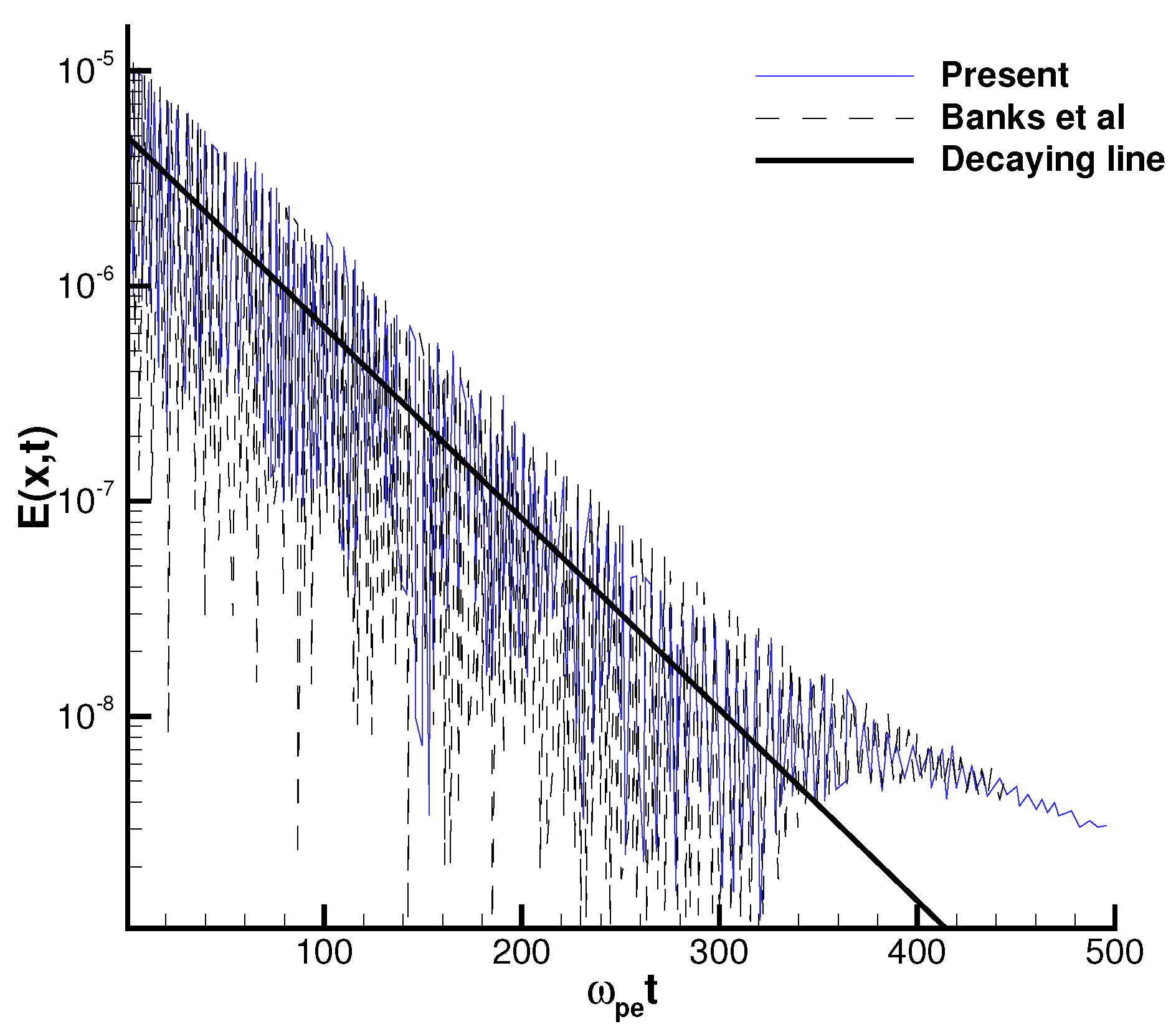
In the EPW case, the wavenumber is set to be 0.3. In the low perturbation amplitude regime, the initial electron distribution is

$$f=\rho \left(\frac{\lambda }{\pi }\right)e^{-\lambda \left({\mathit{u}}^2\right)}\left(1+\alpha \cos \left(kx\right)\right),$$

(48)

where $\alpha =0.0001$ and $k=\frac{\pi }{250}$. The 1D computational domain is discretized with 64 grid points. In microscopic velocity space, 128 discrete points are used. To compared with the result of Reference [57], the thermal electron-ion collision frequency ${\nu }_{ei,th}$ is set to be 0.05. The amplitude of the perturbation’s electric field E is plotted on a log scale as a function of time in Figure 13.

Where ${\omega }_{pe}$ is the circular frequency of initial perturbation. The result obtained from present methods is consistent with Reference [57]. The decaying process fit well with exponential decaying line. Because of the initial perturbation of particle distribution, the electric field is also damped in oscillatory process. In traditional numerical method based on continuous assumption, it is very hard to capture these phenomena for the lack of direct modelling of particle motion. For the particle-based method, the huge number of particles always produces unacceptable computational cost. In UGKS, particle motion is described in modelling of flux through cell interface under discrete microscopic velocity space. For every discrete distribution function, computational cost only comes from reconstruction in flux evaluation. However, its accuracy is the same as particle-based method since all particles are considered based on statistical concept using distribution function. With the suitable collision model, a different state of plasma can be accurately obtained.

4. Conclusions

In this paper, we solve the Boltzmann equation to simulate the plasma flow based on the UGKS. This approach gives a full representation for particle moving in phase space under electric field. An integral solution of the kinetic model under discrete physical and particle velocity space is applied. In non-equilibrium state, this method can describe distribution function with discrete phase space. Compared to Lagrangian method, the UGKS has a much lower computational cost but achieves the same accuracy in plasma simulation. Many methods for solution of the Vlasov equation, such as FEM and spectral method, still have to solve equation of particle motion to decide the coefficients in basis functions for particle velocity dimensions. As a result, the time step is restricted according to dissipative length scale determined by the physical transport. Time step in current work can be decided by CFL strategy without spurious dissipation. In order to simplify the solution of the Poisson’s equation by using the Green’s function, we restrict the boundary conditions to the periodic or symmetric boundary conditions. The method presented in this paper can be used in simulation for plasma flows in electric field. In multi-scale problems of plasma flows from free transport regime to collisional effect, UGKS can give pretty good description of physical evolution. Compared to the particle-based method, computational efficiency has also been greatly improved. Its advantages will make it a promising tool for plasma research.

References

- Vlasov, A. On vibration properties of electron gas. J. Exp. Theor. Phys. 1938, 8, 291. [Google Scholar]
- Merrill, H.J.; Webb, H.W. Electron scattering and plasma oscillations. Phys. Rev. 1939, 55, 1191. [Google Scholar] [CrossRef]
- Degond, P.; Deluzet, F.; Navoret, L.; Sun, A.B.; Vignal, M.H. Asymptotic-preserving particle-in-cell method for the Vlasov–Poisson system near quasineutrality. J. Comput. Phys. 2010, 229, 5630–5652. [Google Scholar] [CrossRef]
- Crouseilles, N.; Mehrenberger, M.; Vecil, F. Discontinuous Galerkin semi-Lagrangian method for Vlasov-Poisson. ESAIM Proc. 2011, 32, 211–230. [Google Scholar] [CrossRef]
- Seal, D.C. Discontinous Galerkin Methods for Vlasov Models of Plasma. Ph.D. Thesis, University of Wisconsin-Madison, Madison, WI, USA, 2012. [Google Scholar]
- Heath, R.; Gamba, I.M.; Morrison, P.J.; Michler, C. A discontinuous Galerkin method for the Vlasov–Poisson system. J. Comput. Phys. 2012, 231, 1140–1174. [Google Scholar] [CrossRef]
- Schumer, J.W.; Holloway, J.P. Vlasov simulations using velocity-scaled Hermite representations. J. Comput. Phys. 1998, 144, 626–661. [Google Scholar] [CrossRef]
- Le Bourdiec, S.; De Vuyst, F.; Jacquet, L. Numerical solution of the Vlasov–Poisson system using generalized Hermite functions. Comput. Phys. Commun. 2006, 175, 528–544. [Google Scholar] [CrossRef]
- Crouseilles, N.; Respaud, T.; Sonnendrücker, E. A forward semi-Lagrangian method for the numerical solution of the Vlasov equation. Comput. Phys. Commun. 2009, 180, 1730–1745. [Google Scholar] [CrossRef]
- Godunov, S. A difference scheme for numerical solution of discontinuous solution of hydrodynamic equations. Mat. Sb. 1959, 47, 271–306. [Google Scholar]
- Sonnendrücker, E.; Roche, J.; Bertrand, P.; Ghizzo, A. The Semi-Lagrangian Method for the Numerical Resolution of the Vlasov Equation. J. Comput. Phys. 1999, 149, 201–220. [Google Scholar] [CrossRef]
- Filbet, F.; Sonnendrücker, E.; Bertrand, P. Conservative numerical schemes for the Vlasov equation. J. Comput. Phys. 2001, 172, 166–187. [Google Scholar] [CrossRef]
- Crouseilles, N.; Latu, G.; Sonnendrücker, E. Hermite spline interpolation on patches for parallelly solving the Vlasov-Poisson equation. Int. J. Appl. Math. Comput. Sci. 2007, 17, 335–349. [Google Scholar] [CrossRef]
- Banks, J.; Berger, R.; Brunner, S.; Cohen, B.; Hittinger, J. Two-Dimensional Vlasov Simulation of Electron Plasma Wave Trapping, Wavefront Bowing, Self-Focusing, and Sideloss. Phys. Plasmas 2011, 18, 052102. [Google Scholar] [CrossRef]
- Xu, S.Y.; Cai, J.S.; Li, J. Modeling and simulation of plasma gas flow driven by a single nanosecond-pulsed dielectric barrier discharge. Phys. Plasmas 2016, 23, 103510. [Google Scholar] [CrossRef]
- Xu, K.; Huang, J.C. A unified gas-kinetic scheme for continuum and rarefied flows. J. Comput. Phys. 2010, 229, 7747–7764. [Google Scholar] [CrossRef]
- Huang, J.C.; Xu, K.; Yu, P. A unified gas-kinetic scheme for continuum and rarefied flows II: Multi-dimensional cases. Commun. Comput. Phys. 2012, 12, 662–690. [Google Scholar] [CrossRef]
- Xu, K.; Huang, J.C. An improved unified gas-kinetic scheme and the study of shock structures. IMA J. Appl. Math. 2011, 76, 698–711. [Google Scholar] [CrossRef]
- Chen, S.; Xu, K.; Lee, C.; Cai, Q. A unified gas kinetic scheme with moving mesh and velocity space adaptation. J. Comput. Phys. 2012, 231, 6643–6664. [Google Scholar] [CrossRef]
- Liu, S.; Zhong, C. Modified unified kinetic scheme for all flow regimes. Phys. Rev. E 2012, 85, 066705. [Google Scholar] [CrossRef] [PubMed]
- Wang, R.J.; Xu, K. The study of sound wave propagation in rarefied gases using unified gas-kinetic scheme. Acta Mech. Sin. 2012, 28, 1022–1029. [Google Scholar] [CrossRef]
- Mieussens, L. On the asymptotic preserving property of the unified gas kinetic scheme for the diffusion limit of linear kinetic models. J. Comput. Phys. 2013, 253, 138–156. [Google Scholar] [CrossRef]
- Liu, S.; Yu, P.; Xu, K.; Zhong, C. Unified gas-kinetic scheme for diatomic molecular simulations in all flow regimes. J. Comput. Phys. 2014, 259, 96–113. [Google Scholar] [CrossRef]
- Liu, S.; Zhong, C. Investigation of the kinetic model equations. Phys. Rev. E 2014, 89, 033306. [Google Scholar] [CrossRef] [PubMed]
- Liu, S.; Zhong, C.; Bai, J. Unified gas-kinetic scheme for microchannel and nanochannel flows. Comput. Math. Appl. 2015, 69, 41–57. [Google Scholar] [CrossRef]
- Chen, S.; Xu, K. A comparative study of an asymptotic preserving scheme and unified gas-kinetic scheme in continuum flow limit. J. Comput. Phys. 2015, 288, 52–65. [Google Scholar] [CrossRef]
- Sun, W.; Jiang, S.; Xu, K. An asymptotic preserving unified gas kinetic scheme for gray radiative transfer equations. J. Comput. Phys. 2015, 285, 265–279. [Google Scholar] [CrossRef]
- Liu, C.; Xu, K.; Sun, Q.; Cai, Q. A unified gas-kinetic scheme for continuum and rarefied flows IV: Full Boltzmann and model equations. J. Comput. Phys. 2016, 314, 305–340. [Google Scholar] [CrossRef]
- Liu, S.; Liang, Y. Asymptotic-preserving Boltzmann model equations for binary gas mixture. Phys. Rev. E 2016, 93, 023102. [Google Scholar] [CrossRef] [PubMed]
- Zhu, Y.; Zhong, C.; Xu, K. Implicit unified gas-kinetic scheme for steady state solutions in all flow regimes. J. Comput. Phys. 2016, 315, 16–38. [Google Scholar] [CrossRef]
- Zhu, Y.; Zhong, C.; Xu, K. Unified gas-kinetic scheme with multigrid convergence for rarefied flow study. Phys. Fluids 2017, 29, 096102. [Google Scholar] [CrossRef]
- Wang, P.; Ho, M.T.; Wu, L.; Guo, Z.; Zhang, Y. A comparative study of discrete velocity methods for low-speed rarefied gas flows. Comput. Fluids 2018, 161, 33–46. [Google Scholar] [CrossRef]
- Xu, K. Gas-Kinetic Schemes for Unsteady Compressible Flow Simulations. In 29th Computational Fluid Dynamics: February 23–27, 1998; Von Karman Institute for Fluid Dynamics: Rhode St. Genèse, Belgium, 1998. [Google Scholar]
- Courant, R.; Friedrichs, K.; Lewy, H. Über die partiellen Differenzengleichungen der mathematischen Physik. Math. Ann. 1928, 100, 32–74. [Google Scholar] [CrossRef]
- Liu, C.; Xu, K. A unified gas-kinetic scheme for continuum and rarefied flows V: Multiscale and multi-component plasma transport. Commun. Comput. Phys. 2017, 22, 1175–1532. [Google Scholar] [CrossRef]
- Courant, R.; Isaacson, E.; Rees, M. On the solution of nonlinear hyperbolic differential equations by finite differences. Commun. Pure Appl. Math. 1952, 5, 243–255. [Google Scholar] [CrossRef]
- Canuto, C.; Hussaini, M.Y.; Quarteroni, A.; Zang, T.A. Spectral Methods: Evolution to Complex Geometries And Applications to Fluid Dynamics; Springer Science & Business Media: Berlin, Germany, 2007. [Google Scholar]
- Wu, L.; Reese, J.M.; Zhang, Y. Oscillatory rarefied gas flow inside rectangular cavities. J. Fluid Mech. 2014, 748, 350–367. [Google Scholar] [CrossRef] [Green Version]
- Sturrock, P.A. Plasma Physics: An Introduction to the Theory of Astrophysical, Geophysical and Laboratory Plasmas; Cambridge University Press: Cambridge, UK, 1994. [Google Scholar]
- Hazeltine, R.D.; Waelbroeck, F.L. The Framework of Plasma Physics; Westview: London, UK, 2004. [Google Scholar]
- Mouhot, C.; Villani, C. Landau damping. J. Math. Phys. 2010, 51, 015204. [Google Scholar] [CrossRef] [Green Version]
- Wu, L.; Reese, J.M.; Zhang, Y. Solving the Boltzmann equation deterministically by the fast spectral method: Application to gas microflows. J. Fluid Mech. 2014, 746, 53–84. [Google Scholar] [CrossRef] [Green Version]
- Tian, C.T.; Xu, K.; Chan, K.L.; Deng, L.C. A three-dimensional multidimensional gas-kinetic scheme for the Navier-Stokes equations under gravitational fields. J. Comput. Phys. 2007, 226, 2003–2027. [Google Scholar] [CrossRef]
- Maxwell, J.C. A Dynamical Theory of the Electromagnetic Field; Scottish Academic Press: Edinburgh, UK, 1982; pp. 459–512. [Google Scholar]
- Christlieb, A.J.; Krasny, R.; Verboncoeur, J.P. Efficient particle simulation of a virtual cathode using a grid-free treecode Poisson solver. IEEE Trans. Plasma Sci. 2004, 32, 384–389. [Google Scholar] [CrossRef]
- Bayin, S. Mathematical Methods in Science and Engineering; John Wiley & Sons: Hoboken, NJ, USA, 2006. [Google Scholar]
- Griffiths, D.J. Introduction to Electrodynamics, 3rd ed.; Pearson Education Asia Limited: Hong Kong, China, 2006. [Google Scholar]
- Huray, P.G. Maxwell’s Equations; John Wiley & Sons: Hoboken, NJ, USA, 2011. [Google Scholar]
- Francis, F.C. Introduction to Plasma Physics and Controlled Fusion: Plasma Physics; Springer: New York, NY, USA, 1984; Volume 1. [Google Scholar]
- Lynden-Bell, D. The stability and vibrations of a gas of stars. Mon. Not. R. Astron. Soc. 1962, 124, 279–296. [Google Scholar] [CrossRef]
- Tsurutani, B.T.; Lakhina, G.S. Some basic concepts of wave-particle interactions in collisionless plasmas. Rev. Geophys. 1997, 35, 491–501. [Google Scholar] [CrossRef]
- Landau, L.D. On the vibrations of the electronic plasma. J. Exp. Theor. Phys. 1946, 10, 24–25. [Google Scholar]
- Degond, P. Spectral theory of the linearized Vlasov-Poisson equation. Trans. Am. Math. Soc. 1986, 294, 435–453. [Google Scholar] [CrossRef]
- Caglioti, E.; Maffei, C. Time asymptotics for solutions of Vlasov–Poisson equation in a circle. J. Stat. Phys. 1998, 92, 301–323. [Google Scholar] [CrossRef]
- Broglie, L.D. The Wave Nature of the Electron. Nobel Lect. 1929, 12, 244–256. [Google Scholar]
- Xu, K. A gas-kinetic BGK scheme for the Navier-Stokes equations and its connection with artificial dissipation and Godunov method. J. Comput. Phys. 2001, 171, 289–335. [Google Scholar] [CrossRef]
- Banks, J.; Brunner, S.; Berger, R.; Tran, T. Vlasov simulations of electron-ion collision effects on damping of electron plasma waves. Phys. Plasmas 2016, 23, 032108. [Google Scholar] [CrossRef]
Figure 1.
Density contour of the linear Landau damping at different time steps under non dimensional axis.
Figure 2.
Evolution of symmetric electric field of the linear Landau damping with non dimensional time.
Figure 3.
Evolution of electric potential energy of the linear Landau damping with non dimensional time.
Figure 4.
Evolution of the kinetic entropy of nonlinear Landau damping with non dimensional time.
Figure 5.
Evolution of -norm of distribution function in nonlinear Landau damping with non dimensional time.
Figure 6.
Non-equilibrium distribution functions at different time steps of nonlinear Landau damping under non dimensional microscopic velocity space.
Figure 7.
Distribution functions of nonlinear Landau damping in phase space at different non dimensional numerical time steps.
Figure 8.
Development of the distribution function at in nonlinear Landau damping case with non dimensional time.
Figure 9.
Development of entropy in nonlinear Landau damping case with non dimensional time.
Figure 10.
Mesh for the simulation of the Gaussian beam under non dimensional physical space.
Figure 11.
Buffer zone and flux on the warp for simulation of the Gaussian beam under non dimensional physical space.
Figure 12.
Density distribution of the Gaussian beam at different non dimensional time steps in non dimensional physical space for particle density.
Figure 13.
Amplitude of the perturbation’s electric field for particle density perturbation .