Thermal Lattice Boltzmann Simulation of Evaporating Thin Liquid Film for Vapor Generation

Featured Application

This work can potentially be used in applications where thin film evaporation is involved, for example, cooling and vapor generation. The approach introduced in this paper may facilitate the phenomenon-level understanding of heat and mass transfer, as well as the device-level design.

Abstract

Thin film evaporation (TFE) plays an important role in many industrial applications, such as power generation, cooling, and thermal management. Effective evaporation takes place in the thin liquid film region with relatively low film thickness and low intermolecular forces. In this paper, a numerical approach based on the thermal lattice Boltzmann method (TLBM) is employed to investigate the heat and mass transfer phenomena in TFE. The TLBM approach is validated by simulating some benchmark problems, and is then used to study a vapor generation problem where TFE is involved. Specifically, vapor is generated from evaporating pores, the solid walls of which are hydrophilic. Factors that affect the overall vapor generation efficiency are investigated via the numerical approach. Methods that can improve the overall efficiency are further proposed. Simulations reveal that distributed scenarios (using distributed small pores instead of a big one) and hydrophobic pore ends render more efficient vapor generation.

1. Introduction

The fast development of microelectronic devices requires advanced thermal management. For devices with large heat flux such as integrated circuits and concentrator solar cells, highly efficient heat transfer approaches are desired. One of the promising solutions that has gained much attention is thin film evaporation (TFE), which can accommodate large heat fluxes owing to liquid-to-vapor phase change. At the contact line between a wetting liquid and solid, there is a thin film region. When the film is ultra thin (usually on the order of 10 nm), the thermal resistance is very small. However, the intermolecular force between liquid and solid is very strong, thus almost no evaporation takes place. This region is called the adhesion film region. On the other hand, the film thickness is relatively large in the intrinsic meniscus region, which results in large thermal resistance and weak evaporation. Hence, most of the evaporation takes place in the region with relatively low thickness and low intermolecular forces. The schematic of evaporating thin film is demonstrated in Figure 1.

Many researchers so far have conducted relevant studies through both theoretical analysis [1,2,3,4] and experimental approaches [5,6,7]. From the theoretical point of view, it is troublesome to solve a sophisticated model that involves complicated partial differential equations. However, some assumptions should be made if a simplified problem is considered instead, which weakens the physical meaning. Since TFE is usually considered in micro-scale and even nano-scale devices, measuring the physical quantities, such as the thickness of liquid film and the local temperature, via experimental methods is also challenging. Besides, it is extremely difficult to go deep into the interfacial phenomena where evaporation takes place. Hence, it is imperative to investigate TFE using simulation approaches. Note that TFE is essentially a multiphase flow problem with heat transfer. There are many approaches that can be used in fluid flow simulations, such as the finite volume method [8], smoothed particle hydrodynamics [9], molecular dynamics (MD) [10], lattice Boltzmann method (LBM) [11], etc. Comparisons of various approaches can be found in [12,13]. In our study of TFE, LBM is mainly considered, which is a mesoscopic computational fluid dynamics approach. It is known that LBM is good at tackling fluid-solid interaction and complex geometries. Besides, LBM employs a simple algorithm (collision and streaming), which makes it intrinsically scalable and parallelizable for computations. LBM has been used in many engineering and scientific problems, e.g., [14,15,16,17,18,19,20]. In this paper, we will show that LBM, and more specifically thermal LBM (TLBM), can reproduce several important phenomena in TFE, even without very fine mesh grids. Hence, it facilitates our understanding of the physics behind TFE and further device-level design.

In the last decade, TLBM has been widely investigated [21]. There are several TLBM approaches, which can be classified as the multispeed method [22], the double distribution method [23], and the hybrid method [24]. A more detailed discussion of various approaches can be found in the excellent review paper [25]. It is noticed that TLBM has been applied in the study of many thermal flow problems, e.g., natural convection [26,27], and boiling [28,29,30]. More recently, the authors of [31] reported results on TFE at a hydrophilic microstructured surface using a double distribution TLBM approach. The surface consists of micro pillars. The influence of wettability and heat flux on liquid film distribution and liquid-vapor interface morphology were investigated. In addition, the dependence of dry-out heat flux and wettability was discussed. In this paper, we also propose a double distribution TLBM approach that is based on a pseudo-potential function. The approach is considered in the study of TFE. We mainly focus on the interfacial phenomena, which may be hardly observed through experimental methods. By introducing some flow and thermal boundary conditions, the proposed method is further applied in the investigation of a practical problem, which is direct vapor generation. Specifically, vapor is generated in evaporating pores where heat is concentrated. TFE is involved in the problem due to the fact that the solid walls of pores are hydrophilic. Factors that affect the overall efficiency of vapor generation are investigated, including the pore distribution and wettability of the solid walls. With the help of TLBM simulations, a scenario that can achieve higher vapor generation efficiency is proposed. As a result, the TLBM approach may facilitate our understanding of the phenomena that relate to TFE, and our design of devices where TFE is involved. Before presenting the main results, the TLBM approach together with some validations are discussed first in the following section.

2. Double Distribution TLBM

The model we consider in our study is the so-called double distribution thermal lattice Boltzmann model (TLBM). It was firstly proposed in [23], where density and energy are considered in different distribution functions. A TLBM approach was further developed in [32] with quantitative analysis, which also inspires the modeling employed in this work.

2.1. Density Distribution Function

The D2Q9 lattice Boltzmann (LB) model has been widely used in simulations of many complex flows [33]. It consists of two parts, namely streaming and collision. A D2Q9 model with Bhatnagar-Gross-Krook approximation of the collision term is given by

$$f_i(\mathbf{x}+\Delta \mathbf{x},t+\Delta t)=f_i(\mathbf{x},t)-\frac{1}{{\tau }_f}[f_i(\mathbf{x},t)-f_i^{\mathrm{eq}}(\mathbf{x},t)]+\Delta f_i(\mathbf{x},t),$$

(1)

where $f_i(\mathbf{x},t)$ is the particle distribution function in the i-th discretized velocity direction at position $\mathbf{x}$ and time t, $\Delta x$, $\Delta t$ and ${\tau }_f$ are the lattice spacing, time step and relaxation time, respectively. The equilibrium distribution function is obtained by

$$f_i^{\mathrm{eq}}=\rho w_i\left[1+\frac{{\mathbf{e}}_i·\mathbf{u}}{c_{s^2}}+\frac{{({\mathbf{e}}_i·\mathbf{u})}^2-(c_s{\left|\mathbf{u}\right|)}^2}{2c_s^2}\right],$$

(2)

and one has

$$\Delta f_i=f_i^{\mathrm{eq}}(\rho ,\mathbf{u}+\Delta \mathbf{u})-f_i^{\mathrm{eq}}(\rho ,\mathbf{u}),$$

(3)

with $w_0=4/9$, $w_{1,2,3,4}=1/9$, $w_{5,6,7,8}=1/36$, $c_s=\sqrt{3}c$ the sound speed, $c=\Delta x/\Delta t$, $\mathbf{u}={\sum }_{i=0}^8{f}_i{\mathbf{e}}_i$, and the velocity set ${\mathbf{e}}_i$ is given by

$${\mathbf{e}}_i=\left(e_x\left(i\right),e_y\left(i\right)\right)=\left\{\begin{array}{cc}(0,0)c\hfill & i=0\hfill \\ (cos[(i-1)\frac{\pi }{2}],sin[(i-1)\frac{\pi }{2}])c\hfill & i=1,2,3,4\hfill \\ (\sqrt{2}cos[(2i-9)\frac{\pi }{4}],\sqrt{2}sin[(2i-9)\frac{\pi }{4}])c\hfill & i=5,6,7,8.\hfill \end{array}\right.$$

(4)

Letting $\mathbf{F}$ be an external force, then the macroscopic properties such as density and velocity can be obtained by

$$\rho (\mathbf{x},t)=\sum _{i=0}^8{f}_i(\mathbf{x},t),\mathbf{U}(\mathbf{x},t)=\mathbf{u}(\mathbf{x},t)+\frac{1}{2}\frac{\mathbf{F}(\mathbf{x},t)}{\rho (\mathbf{x},t)}.$$

(5)

Furthermore, the kinematic viscosity $\nu$ relates to the relaxation time by $\nu =(\tau -0.5)c_s^2\Delta t$. The exact difference method shown as above has good performance in simulating multiphase flows due to its simplicity and accuracy [34]. Moreover, the unphysical influence of relaxation time can be avoided. In the TFE problem, the external forces $\mathbf{F}$ include cohesive force (between fluid nodes), adhesion force (between fluid and solid nodes), and body force (e.g. gravity). They will be discussed in the following.

A single component multiphase LB model is considered to investigate TFE. Numerous results on the multiphase LB model have been reported. Readers may refer to [21,25,35] and the references therein for more detailed information. A pseudopotential approach inspired by [32,36] is considered in this work. The cohesive force is described as the gradient of a psudopotential function, which has the following form

$$\varphi =-G(\rho c_s^2-\beta P),$$

(6)

where P is the pressure, G and $\beta$ are two tuning parameters. As studied in [32], the parameter $\beta$ controls the resolution of liquid-vapor interface. Note that high resolution, however, suffers from numerical instability. The parameter G affects the density ratio of liquid and vapor. The model reduces to the one discussed in [32] as G equals 1. It is worth mentioning that the pseudopotential function can accommodate different equation of states (EOS). In our study, the normalized Van der Waals EOS is considered, that is

$$P=\frac{8\rho T}{3-\rho }-3{\rho }^2.$$

(7)

In the above equation, the dimensionless physical variables are defined as

$$\rho =\frac{\widehat{\rho }}{{\widehat{\rho }}_c},P=\frac{\widehat{P}}{{\widehat{P}}_c},T=\frac{\widehat{T}}{{\widehat{T}}_c},$$

(8)

where $\widehat{\rho }$, $\widehat{P}$, and $\widehat{T}$ denote the density, pressure, and temperature in physical units, respectively, while ${\widehat{\rho }}_c$, ${\widehat{P}}_c$, and ${\widehat{T}}_c$ correspond to the critical point. Throughout this paper, the normalized variables which are intrinsically dimensionless will be used in the lattice Boltzmann model.

The pseudopotential function $\varphi (\rho ,T)$ is now obtained by substituting the pressure expression (7) into Equation (6). The cohesive force between fluid nodes is then expressed as

$${\mathbf{F}}_{\mathrm{int}}=-\nabla \varphi (\rho ,T).$$

(9)

Note that in the computation of ${\mathbf{F}}_{\mathrm{int}}$, a discretized realization of gradient is required. The two-dimensional gradient $\nabla \varphi$ can be approximated by

$$\nabla \varphi (\mathbf{x},t)\approx \frac{1}{c\Delta x}\sum _{i=1}^8{\lambda }_i\varphi (\mathbf{x}+{\mathbf{e}}_i\Delta t,t){\mathbf{e}}_i,$$

(10)

where ${\lambda }_{1,2,3,4}=4/12$ and ${\lambda }_{5,6,7,8}=1/12$ [32]. On the other hand, we may define $\psi$ as $\sqrt{2\varphi }$. Then $\nabla \varphi$ can also be approximated as

$$\nabla \varphi (\mathbf{x},t)\approx \frac{1}{c\Delta x}\psi (\mathbf{x},t)\sum _{i=1}^8{\lambda }_i\psi (\mathbf{x}+{\mathbf{e}}_i\Delta t,t){\mathbf{e}}_i,$$

(11)

Based on Equations (10) and (11), an improved method is developed [34],

$$\nabla \varphi (\mathbf{x},t)\approx \frac{1}{c\Delta x}\left[A\psi (\mathbf{x},t)\sum _{i=1}^8{\lambda }_i\psi (\mathbf{x}+{\mathbf{e}}_i\Delta t,t){\mathbf{e}}_i+(1-A)\sum _{i=1}^8{\lambda }_i\varphi (\mathbf{x}+{\mathbf{e}}_i\Delta t,t){\mathbf{e}}_i\right].$$

(12)

In the above approximation of gradient, A is a weighting factor. For Van der Waals EOS, it is suggested that A = 0.55 gives good performance [34]. Note that when the neighbor of a fluid node is solid, the adhesion force should be considered. A convenient way is to assign the density and temperature for solid nodes, denoted as ${\rho }_{\mathrm{w}}$ and $T_{\mathrm{w}}$. Now the cohesive force and the adhesion force can be jointly given by

$${\mathbf{F}}_{\mathrm{int}}+{\mathbf{F}}_{\mathrm{ad}}=-\nabla \varphi (\rho ,T).$$

(13)

If a body force ${\mathbf{F}}_{\mathrm{g}}$ exists, e.g., gravity, then the total force is

$$\mathbf{F}={\mathbf{F}}_{\mathrm{g}}-\nabla \varphi (\rho ,T).$$

(14)

It is worth mentioning that solid nodes are assigned with ${\rho }_{\mathrm{w}}$ only when we calculate the adhesion force. That is to say, ${\rho }_{\mathrm{w}}$ does not affect the density distribution function in the streaming and collision processes.

2.2. Energy Distribution Function

In the double distribution LB model, an energy distribution function is considered independent of the density distribution in order to mimic the energy transport. The following energy distribution function is employed in our study

$$g_i(\mathbf{x}+\Delta \mathbf{x},t+\Delta t)-g_i(\mathbf{x},t)=-\frac{1}{{\tau }_g}(g_i(\mathbf{x},t)-g_i^{\mathrm{eq}}(\mathbf{x},t))$$

(15)

where $g_i(\mathbf{x},t)$ is the energy distribution in the i-th discretized direction, and ${\tau }_g$ is the relaxation time for energy. The equilibrium distribution $g_i^{\mathrm{eq}}$ is defined as

$$\begin{array}{ccc}\hfill g_0^{\mathrm{eq}}& =& -\frac{2\rho c_{v}T}{3}\frac{{\mathbf{U}}^2}{c^2},\hfill \end{array}$$

(16)

$$\begin{array}{ccc}\hfill g_{1,2,3,4}^{\mathrm{eq}}& =& \frac{\rho c_{v}T}{9}[\frac{3}{2}+\frac{3{\mathbf{e}}_i·\mathbf{U}}{2c^2}+\frac{9{({\mathbf{e}}_i·\mathbf{U})}^2}{2c^4}-\frac{3{\mathbf{U}}^2}{2c^2}],\hfill \end{array}$$

(17)

$$\begin{array}{ccc}\hfill g_{5,6,7,8}^{\mathrm{eq}}& =& \frac{\rho c_{v}T}{36}[3+\frac{6{\mathbf{e}}_i·\mathbf{U}}{c^2}+\frac{9{({\mathbf{e}}_i·\mathbf{U})}^2}{2c^4}-\frac{3{\mathbf{U}}^2}{2c^2}].\hfill \end{array}$$

(18)

In the above equations, $c_v$ is the heat capacity at constant volume (assumed to be 1 in our study). This model differs from the one proposed in [23], where both viscous dissipation and the compression work done by the pressure were taken into account. The influence of viscous dissipation can be evaluated via the Brinkman number Br, which is defined as $\mathrm{Br}=\nu {\mathbf{u}}^2/(\alpha T_0-\alpha T)$, where $T_0$ and T represent temperature of wall and fluid, respectively. The importance of compression work is reflected by the Mach number, that is $\mathrm{Ma}=\left|\mathbf{U}\right|/c_s$. In the problem of TFE, both Br and Ma are usually very small. Hence, viscous dissipation and compression work are negligible in our study. The resulting energy distribution function is significantly simplified. Furthermore, the second order truncation error can be absorbed in the relaxation time ${\tau }_f$ and ${\tau }_g$. It is noticed that for the multiphase flow, the density difference between liquid and vapor phases is large, which deteriorates the numerical stability in the thermal flow simulations. Hence, another variable $g^{\prime }$ is introduced, that is $g^{\prime }=g/\rho$. Now $g^{\prime }$ is considered in the steaming and collision steps. Furthermore, the equilibrium distribution of $g_i^{\prime }$ can easily be extracted from Equations (16)–(18). The temperature T is then computed via

$$T=\sum _{i=0}^8{g}_i^{\prime }.$$

(19)

The thermal diffusivity $\alpha$ is expressed as $\alpha =2c_s^2({\tau }_g-0.5)\Delta t$.

2.3. Boundary Conditions

Boundary conditions have great influence on the numerical simulations. Abundant achievements have been reported for the flow field. The classic bounce-back scheme is a simple treatment for the non-slip boundary condition. Bounce back combined with specular refection can generate slip boundary condition [11]. Other popular boundary conditions include Zou and He’s non-equilibrium bounce-back method [37] and Guo’s extrapolation method [38], etc. The results relating to thermal boundary conditions are relatively fewer. In the following part, we will first discuss the thermal boundary conditions. After that, a replenishment boundary condition is introduced, which will be employed in our study of the vapor generation problem.

2.3.1. Thermal Boundary Conditions

We mainly focus on two types of thermal boundary conditions, namely constant temperature and constant heat flux. The constant temperature boundary condition is considered first. The south wall shown in Figure 2 is taken as an example, the temperature of which is constant, denoted as $T_0$. The energy distributions $g_2^{\prime }$, $g_5^{\prime }$ and $g_6^{\prime }$ are unknown after the streaming process. It is assumed that $g_2^{\prime }$, $g_5^{\prime }$ and $g_6^{\prime }$ follow equilibrium distributions. The idea comes from the “counter-slip” approach proposed in [39]. Similar consideration can be found in [26,40,41,42]. It is mentioned in [26] that this treatment provides significant numerical stability and accuracy. For the three unknown distributions it holds

$$\begin{array}{ccc}\hfill g_2^{\prime }& =& \frac{T^{\prime }}{9}[\frac{3}{2}+\frac{3{\mathbf{e}}_2·{\mathbf{u}}_{\mathrm{w}}}{2c^2}+\frac{{(9{\mathbf{e}}_2·{\mathbf{u}}_{\mathrm{w}})}^2}{2c^4}-\frac{3{\mathbf{u}}_{\mathrm{w}}^2}{2c^2}],\hfill \end{array}$$

(20)

$$\begin{array}{ccc}\hfill g_5^{\prime }& =& \frac{T^{\prime }}{36}[3+\frac{6{\mathbf{e}}_5·{\mathbf{u}}_{\mathrm{w}}}{c^2}+\frac{{(9{\mathbf{e}}_5·{\mathbf{u}}_{\mathrm{w}})}^2}{2c^4}-\frac{3{\mathbf{u}}_{\mathrm{w}}^2}{2c^2}],\hfill \end{array}$$

(21)

$$\begin{array}{ccc}\hfill g_6^{\prime }& =& \frac{T^{\prime }}{36}[3+\frac{6{\mathbf{e}}_6·{\mathbf{u}}_{\mathrm{w}}}{c^2}+\frac{{(9{\mathbf{e}}_6·{\mathbf{u}}_{\mathrm{w}})}^2}{2c^4}-\frac{3{\mathbf{u}}_{\mathrm{w}}^2}{2c^2}],\hfill \end{array}$$

(22)

where $T^{\prime }$ is a virtual temperature and ${\mathbf{u}}_{\mathrm{w}}$ is the wall velocity. On the other hand we have

$$\sum _{i=0}^8{g}_i^{\prime }=T_0,$$

(23)

which yields

$$g_2^{\prime }+g_5^{\prime }+g_6^{\prime }=T_0-\sum _{i=0,1,3,4,7,8}{g}_i^{\prime }.$$

(24)

Let ${\gamma }_2$, ${\gamma }_5$ and ${\gamma }_6$ be the weights in Equations (20)–(22) such that

$$g_2^{\prime }={\gamma }_2{T}^{\prime },g_5^{\prime }={\gamma }_5{T}^{\prime },g_6^{\prime }={\gamma }_6{T}^{\prime }.$$

Then it holds

$$\begin{array}{ccc}\hfill g_2^{\prime }& =& \frac{{\gamma }_2}{{\gamma }_2+{\gamma }_5+{\gamma }_6}(T_0-\sum _{i=0,1,3,4,7,8}{g}_i^{\prime }),\hfill \end{array}$$

(25)

$$\begin{array}{ccc}\hfill g_5^{\prime }& =& \frac{{\gamma }_5}{{\gamma }_2+{\gamma }_5+{\gamma }_6}(T_0-\sum _{i=0,1,3,4,7,8}{g}_i^{\prime }),\hfill \end{array}$$

(26)

$$\begin{array}{ccc}\hfill g_6^{\prime }& =& \frac{{\gamma }_6}{{\gamma }_2+{\gamma }_5+{\gamma }_6}(T_0-\sum _{i=0,1,3,4,7,8}{g}_i^{\prime }).\hfill \end{array}$$

(27)

In a special case that the wall is stationary, we have ${\gamma }_2=1/6$ and ${\gamma }_5={\gamma }_6=1/12$.

Now we consider the constant heat flux boundary condition at the normal direction of the south wall. The heat flux can be represented as [41]

$$\mathbf{q}(\mathbf{x},t)=\sum _{i=0}^8({\mathbf{e}}_i-{\mathbf{u}}_{\mathrm{w}})g_i(\mathbf{x},t).$$

(28)

Assume that the heat flux is $q_0$. Then one has

$$\sum _{i=2,5,6}(1-u_{\mathrm{wn}}){\rho }_{\mathrm{w}}{g}_i^{\prime }=q_0-\sum _{i=4,7,8}(-1-u_{\mathrm{wn}}){\rho }_{\mathrm{w}}{g}_i^{\prime },$$

(29)

where $u_{\mathrm{wn}}$ is normal velocity (in the y direction) of the wall. Thus

$$g_2^{\prime }+g_5^{\prime }+g_6^{\prime }=\frac{q_0/{\rho }_{\mathrm{w}}-(-1-u_{\mathrm{wn}}){\sum }_{i=4,7,8}{g}_i^{\prime }}{(1-u_{\mathrm{wn}})}.$$

(30)

It is also assumed that the unknown ones follow an equilibrium distribution. Similarly, $g_2^{\prime }$, $g_5^{\prime }$ and $g_6^{\prime }$ can be obtained from

$$\begin{array}{ccc}\hfill g_2^{\prime }& =& \frac{{\gamma }_2}{{\gamma }_2+{\gamma }_5+{\gamma }_6}·\frac{q_0/{\rho }_{\mathrm{w}}-(-1-u_{\mathrm{wn}}){\sum }_{i=4,7,8}{g}_i^{\prime }}{(1-u_{\mathrm{wn}})},\hfill \end{array}$$

(31)

$$\begin{array}{ccc}\hfill g_5^{\prime }& =& \frac{{\gamma }_5}{{\gamma }_2+{\gamma }_5+{\gamma }_6}·\frac{q_0/{\rho }_{\mathrm{w}}-(-1-u_{\mathrm{wn}}){\sum }_{i=4,7,8}{g}_i^{\prime }}{(1-u_{\mathrm{wn}})},\hfill \end{array}$$

(32)

$$\begin{array}{ccc}\hfill g_6^{\prime }& =& \frac{{\gamma }_6}{{\gamma }_2+{\gamma }_5+{\gamma }_6}·\frac{q_0/{\rho }_{\mathrm{w}}-(-1-u_{\mathrm{wn}}){\sum }_{i=4,7,8}{g}_i^{\prime }}{(1-u_{\mathrm{wn}})}.\hfill \end{array}$$

(33)

Note that the boundary conditions developed above are not restricted to solid nodes. They are also applicable to fluid nodes. Apart from the approaches presented above, some other thermal boundary conditions can also be found in the literature, for example, the non-equilibrium extrapolation method [43]. The detailed flow and thermal boundary conditions that are employed in our study will be mentioned in specific problems.

2.3.2. Replenishment Boundary Condition

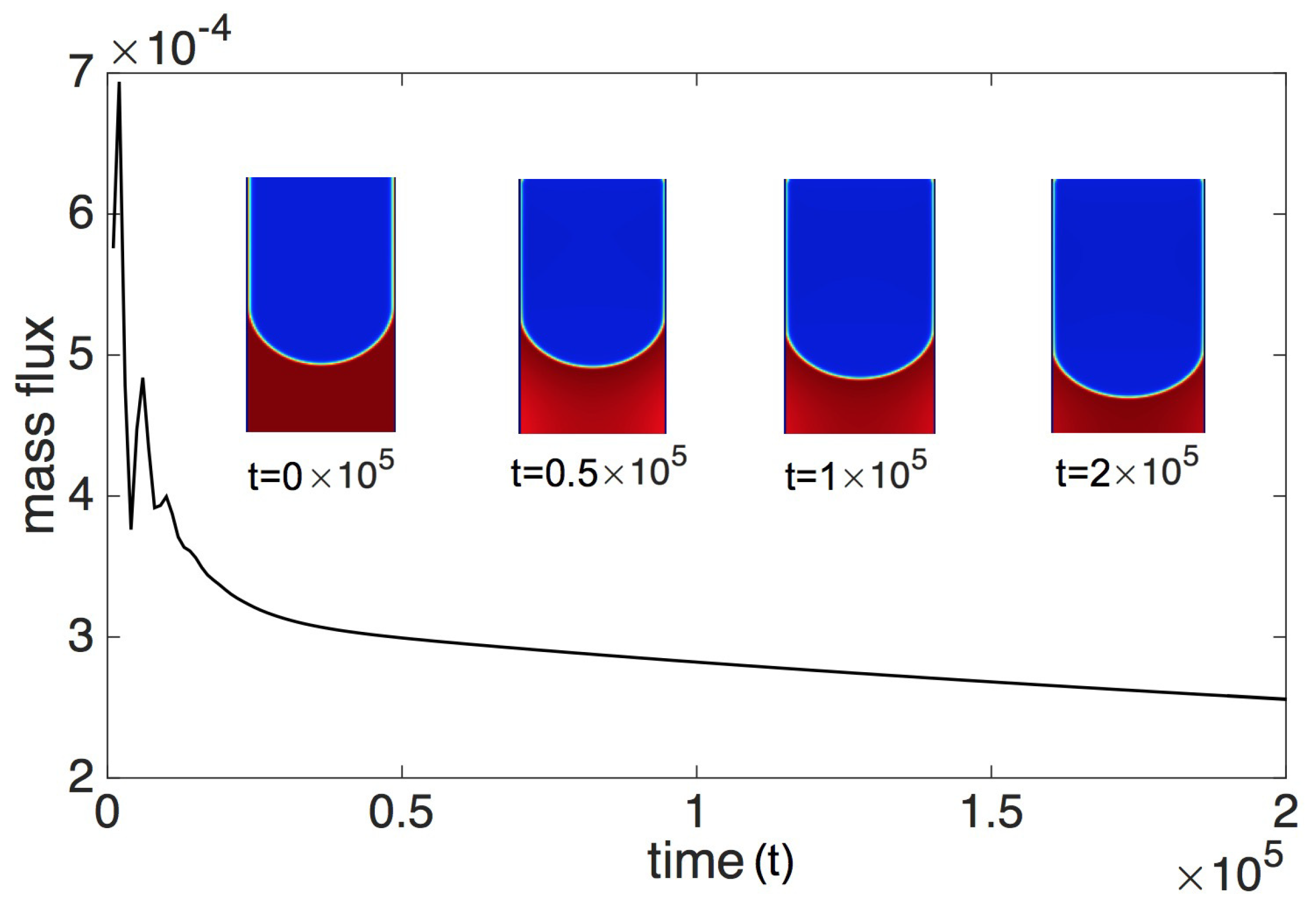
Without replenishment, the liquid level of an evaporating pore will decrease when the solid walls of the pore are constantly heated. The liquid will dry out eventually. As shown in Figure 3, the mass flux at the vapor outlet also decreases during this process. However, in a practical application that involves TFE, the liquid is usually replenished from liquid bulk via the capillary force. We propose to use a ghost layer outside the liquid inlet to replenish the liquid. In other words, the ghost layer serves as the reservoir to supply the liquid. Denote the total mass in the pore as $m_{\mathrm{p}}$. At each time step in the simulation, the loss mass caused by evaporation is estimated by

$$m_{\mathrm{l}}\left(t\right)=m_{\mathrm{p}}-m_{\mathrm{t}}\left(t\right),$$

(34)

where $m_{\mathrm{t}}$ and $m_{\mathrm{l}}$ are the total mass and loss mass, respectively. Then the ghost layer is assigned with the loss mass. Specifically, for each node of the ghost layer, denoted as ${\mathbf{x}}_{\mathrm{gh}}$, the unknown distributions (assume to be $f_2$, $f_5$ and $f_6$) are given by

$$f_i({\mathbf{x}}_{\mathrm{gh}},t)=w_i\frac{m_{\mathrm{l}}\left(t\right)}{W},i=2,5,6.$$

(35)

The effectiveness of the proposed strategy is revealed in Figure 4. It is observed that at the steady state, both total mass and evaporating mass flux are constant. At this point, we have derived a TLBM approach that is able to investigate TFE in an evaporating pore with liquid replenishment.

2.4. Contact Angle and Density Ratio

In this subsection, we will show that both the contact angle and density ratio can be modified in the model. Note that contact angle and density ratio in multiphase LBM approaches have been intensively studied [21]. More recent work can be found as [44], where high density ratio (liquid to vapor) is achieved using the multiphase model of Lee [45]. The main difference of our work is that temperature field is included which brings extra difficulties, for example, thermal fluid simulations are more susceptible to the numerical instability. This section shows that our TLBM approach is able to modify the contact angle and the density ratio even when the flow and temperature field are coupled. The contact angle is investigated first, which relates to the surface wettability. By changing the density of solid nodes, a different contact angle is obtained. Specifically, hydrophilic surface and hydrophobic surface are achieved by choosing ${\rho }_{\mathrm{w}}$ that is close to the liquid density and vapor density, respectively. Figure 5 demonstrates how contact angle changes with ${\rho }_{\mathrm{w}}$, where the temperature T is set as 0.7. It is observed that the contact angle can be modified within a large range.

Different from contact angle, density ratio of liquid and vapor can be influenced by several factors, for example, G, $\alpha$ and T. The dependencies of density ratio on G and $\alpha$ are illustrated in Figure 6. It is observed that the density ratio is mainly determined by the parameter G. With the increase of G, density ratio increases significantly. Compared with G, the parameter $\alpha$ contributes slightly to the density ratio. However, it plays a critical role in the sharpness of liquid-vapor interface. A larger $\alpha$ renders sharper interface, but also makes it vulnerable to numerical instability. Thus a moderate $\alpha$ is suggested in the simulations. Another factor that affects the density ratio is the temperature T. When T increases, both liquid and vapor will have smaller density. Note that the vapor is much more sensitive in the density change with respect to the temperature compared with liquid. As a result, the density ratio is also dependent on temperature.

As a conclusion, the thermal lattice Boltzmann model used in our study is able to mimic different wettabilities. The solid surface can be hydrophilic or hydrophobic. Moreover, the density ratio of liquid and vapor ranges from less than 10 to several hundreds, depending on the parameters of the model.

3. Validations of the TLBM Approach

There are many applications in which TFE occurs in microscale pores. In this section we mainly investigate TFE in a pore using the TLBM approach. The structure illustrated in Figure 7 represents a pore in our simulations. The solid walls are hydrophilic, which ensures that there is a thin-film evaporating region. TFE occurs when the solid walls are heated. We will investigate the thin-film evaporating pore in several aspects, including validations from both reported experiments and theories.

3.1. Wall Temperature Distribution

It is known that heat can be removed through evaporation. Since stronger evaporation occurs in the thin-film evaporating region, a local cooling effect can be expected. Based on this idea, the authors of [5] investigated the wall-temperature distribution of an evaporating micro channel. The wall was heated at constant power in their experiments. The structure shown in Figure 7 is employed to simplify the problem. The domain size in the computation is $67\times 200$ ($x\times y$) in lattice unit. At the inlet of the liquid, we assume that the net mass flow is zero. To this end, we simply use $f_2=f_4,f_5=f_7,f_6=f_8$. At the vapor outlet, the Zou-He boundary condition is employed for the flow field. In the flow field, for the solids nodes, i.e., nodes representing the solid walls, bounce-back rule is adopted, which also applies to all the simulations presented in this paper. For the temperature field, the non-equilibrium extrapolation method is used in both inlet and outlet. Besides, the solid walls are heated at the heat flux $8\times {10}^{-4}$, and thus the constant heat flux boundary condition is considered. Other parameters in the model are $G=0.92$, $\beta =0.06$, and ${\rho }_{\mathrm{s}}=1.9$ (the resulting intrinsic contact angle is about ${15}^{\circ }$). The comparison of TLBM simulations and the experimental data extracted from [5] is given in Figure 8, where X denotes the normalized distance ranging from intrinsic meniscus region ($X=0$) to adsorption region ($X=1$). Thus the thin-film evaporating region locates in the middle. The temperature is normalized via $(T-T_{min})/(T_{max})$, where $T_{min}$ and $T_{max}$ are the minimum and maximum values in the temperature field, respectively. The results shows that the TLBM simulations agree well with the reported experimental data. It is noticed that there is a sudden drop of temperature in the wall temperature distribution, which implies that the intensive evaporation occurs in this region. In our simulations, it is validated that for the same computational domain, mesh resolution larger than $50\times 150$ is fine enough to obtain grid-independent numerical results.

3.2. Evaporating Mass Flux

Evaporating mass flux indicates the capability of evaporation heat transfer. In this part, the mass flux in a thin-film evaporating pore is investigated using TLBM, and is then compared with the theoretical predictions. Schrage proposed that the interfacial mass flux can be estimated by the following equation [46,47],

$$m^{″}=\frac{2\widehat{\sigma }}{2-\widehat{\sigma }}\left(\frac{M}{2\pi R}\right)\left(\frac{P_{v_{eq}}(T_{lv})}{T_{lv}^{1/2}}-\frac{P_v}{T_v^{1/2}}\right),$$

(36)

where $\widehat{\sigma }$ is an accommodation ratio, M is the molecular weight, R is the universal gas constant, $T_{lv}$ is the interface temperature, $P_{v_{eq}}$ is the equilibrium vapor pressure associating with the temperature $T_{lv}$, $P_v$ and $T_v$ are the pressure and temperature of vapor, respectively. The above equation was derived from the kinetic theory. Denote J as the following expression

$$J=\frac{P_{v_{eq}}(T_{lv})}{T_{lv}^{1/2}}-\frac{P_v}{T_v^{1/2}}.$$

(37)

Then mass flux is proportional to J [31], i.e.,

$$m^{″}\propto J.$$

(38)

In the TLBM simulations investigating the evaporating mass flux, the schematic and boundary conditions introduced in the previous part are still employed. The heat flux applied to the side walls changes from $1\times {10}^{-4}$ to $8\times {10}^{-4}$. Hence, different evaporation mass fluxes are achieved. The temperature and pressure in the centre line of the channel are evaluated in order to obtain J as well as the theoretical prediction of $m^{″}$. On the other hand, the mass flux of vapor exiting the pore can also be calculated via

$$m^{″}=\sum _{\mathbf{x}\in {\mathbf{x}}_{\mathrm{out}}}\sum _{i=0}^8{e}_{y,i}{f}_i(\mathrm{x})/W,$$

(39)

where W is the channel width, $e_{y,i}$ is the component of ${\mathbf{e}}_i$ at the y direction, and ${\mathbf{x}}_{\mathrm{out}}$ is the set of nodes locating at the outlet layer. The above equation evaluates the evaporating mass flux directly from the numerical simulations. The comparisons of simulations and theoretical predictions are illustrated in Figure 9, which yields good agreement.

The mass flux discussed above corresponds to an ensemble property of the evaporating pore. It is of interest to look into the details of the liquid-vapor interface, which is an advantage of TLBM. Denote the unit normal vector of the interface as ${\widehat{\mathbf{n}}}_{\mathrm{i}}$. The local mass flux across the interface is estimated by

$$m_{\mathrm{i}}^{″}\left(\mathbf{x}\right)=\sum _{i=0}^8{e}_{y,i}{f}_i\left(\mathbf{x}\right){\widehat{\mathbf{n}}}_{\mathrm{i}}\left(\mathbf{x}\right).$$

(40)

The simulations for interfacial mass flux is shown in Figure 10, where the red solid line represents the contact line throughout adhesion, evaporating and intrinsic meniscus regions. Maximum interfacial mass flux is observed in the evaporating region compared with the adhesion region and the intrinsic meniscus region. It coincides with the classic understanding of TFE.

4. Simulation of Direct Vapor Generation

In this section we will focus on the characterization and optimal design of a vapor generation device that utilizes solar energy. The schematic is illustrated in Figure 11. A device-level design has been accomplished in Massachusetts Institute of Technology (MIT) [48]. The device is a cylinder with a small slot cut in the middle. The absorber is on the top surface of the device, which collects the solar energy under one sun illumination. The bottom of the device is connected to the bulk liquid where water is replenished. As the pore size reduces, solar energy in the pores is more concentrated, which makes it easier for evaporation. Thermal concentration $C_{\mathrm{th}}$ which is defined as the ratio of the whole surface area to the pore area can be used in the evaporating pore problem. Specifically, $C_{\mathrm{th}}=1/(1-\mathsf{\Gamma })$, where $\mathsf{\Gamma }$ is the ratio of absorber area to the whole surface area (usually $\mathsf{\Gamma }\ge 0.98$).

In order to facilitate the evaporation, hydrophilic solid wall is considered for an evaporating pore, which renders TFE. The TLBM approach introduced in this paper is employed to investigate the vapor generation problem. To simplify the problem, it is assumed that the solar power collected by the absorber, denoted as $Q_{\mathrm{a}}$, is described by

$$Q_{\mathrm{a}}=q_{\mathrm{in}}S\mathsf{\Gamma },$$

(41)

where $q_{\mathrm{in}}$ is the incident power density, S is the total surface area (absorber plus pore). Furthermore, we assume that solar energy absorbed by the absorber is concentrated to the solid walls of pores. In the following, we will first consider the influence of pore size to a single evaporating pore.

4.1. Single Pore Scenario

The problem is investigated using the TLBM approach. In the simulations, the depth of pore is fixed as 400$\Delta x$, and the width of the pore varies according to the pore size. It is assumed that the total surface is $2\times {10}^4\Delta x$. Hence, $\mathsf{\Gamma }>0.98$ implies that the pore width is less than 400$\Delta x$. In our simulations, the heat flux density $q_{\mathrm{in}}$ is set to be $1\times {10}^{-4}$. The constant heat flux boundary condition is applied to the solid walls of the pore. By changing the pore width and adopting the corresponding heat flux at the solid walls according to Equation (41), scenarios with various pore width are realized. Since the vapor outlet is connected to the ambient, a constant density and temperature corresponding to the ambient are assumed for the boundary layer of the outlet. At the inlet of the pore, the replenishment boundary condition is considered for the flow field, and a constant temperature boundary condition is employed for the temperature field. We mainly focus on the overall efficiency, which is then compared with the experimental data reported in [48].

The overall efficiency $\eta$ is an important performance index for vapor generation devices. It is defined as the ratio of enthalpy change in the generated vapor to the incident solar power, that is

$$\eta =\frac{\dot{m}{h}_{fg}}{Q_a},$$

(42)

where $\dot{m}$ is the mass flow rate and $h_{fg}$ is the specific enthalpy change of water (from liquid to vapor). When the dimensionless Van der Waals EOS is considered, the enthalpy h is expressed as [32]

$$h=4T\left(\frac{5-\rho }{3-\rho }\right)-6\rho .$$

(43)

And $h_{fg}$ is obtained via its definition, that is

$$h_{fg}=h{|}_{\mathrm{vapor}}-h{|}_{\mathrm{liquid}}.$$

(44)

The comparison between the experimental data reported in [48] and simulation results is shown in Figure 12. Note that in experiments, the estimation of efficiency takes into account the conduction and radiation losses of the device, which are ignored in simulations. In other words, TLBM simulation studies the ideal case. It is observed that the efficiency decreases as the thermal concentration keeps increasing. According to Equation (42), efficiency is mainly dominated by the mass flow rate $\dot{m}$, since the input power $Q_a$ and the enthalpy change $h_{fg}$ does not vary much. Hence, we have the following relationship

$$\eta \propto f_{\mathrm{e}}{A}_{\mathrm{e}},$$

(45)

where $f_{\mathrm{e}}$ is the mass flux of vapor, and $A_{\mathrm{e}}$ is the surface area for evaporation. In our two-dimensional study, $A_{\mathrm{e}}$ is the channel width. The above relationship is also plotted in Figure 12 as a comparison with both simulations and experimental data.

4.2. Multiple Pores Scenario

In the previous part, the case of a single evaporating pore is mainly studied. It is shown that the pore size plays a crucial role in the overall efficiency. Note that the thin-film evaporating region is more efficient in vapor generation compared with the bulk region. Efficiency can thus be further improved if we increase the portion of the thin-film evaporating region. To this end, scenarios with multiple pores are considered in the following part. Specifically, the total pore size is fixed (fixed thermal concentration), while the pore number varies. In other words, more pores imply a smaller size for each one. We still focus on the two-dimensional model. Let L be the width of the absorber, and C as the thermal concentration. Then the total pore size is $L/C$. In the case that n identical pores are considered, the width for each pore is $L/\left(Cn\right)$. Similar to the single pore scenario case, L is chosen as $2\times {10}^4\Delta x$. For example, the thermal concentration is 50, i.e., the width is 400 $\Delta x$ when $n=1$. In order to investigate how the pore number affects the overall efficiency, a consistent heat flux boundary condition is considered in the simulations of different scenarios. The overall efficiency is given by

$$\eta =n\frac{\dot{m_n}{h}_{fg}}{Q_a},$$

(46)

where ${\dot{m}}_n$ is the mass flow rate of the vapor generated in each pore. The results are shown in Figure 13. When the number of pores increases, the overall efficiency will increase first and then decrease. In other words, maximum efficiency exists which corresponds to a moderate number of pores. For more distributed scenarios, the area of thin-film evaporating region is larger, though the total pore area is the same. As a result, the overall efficiency increases. When the number of pores keeps increasing, the pore size becomes very small. Although the thin-film evaporating region still increases, the water supplement could be slugged due to the suppressed viscosity, which reduces the evaporating mass flow rate. This phenomenon was reported in [49], where it is mentioned that, pores with diameters less that 300 nm can hinder water evaporation. Conditions with various incident power are also shown in Figure 13, specifically, $q_{\mathrm{in}}=1\times {10}^{-4}$ and $q_{\mathrm{in}}=1.2\times {10}^{-4}$ are demonstrated. It is revealed that when the incident power is larger, the overall efficiency is also higher. The difference is more obvious for scenarios with more distributed pores. However, it is also noticed that the peak position keeps the same, specifically, $n=11$ renders the maximum efficiency in our simulations.

Another factor that may affect the overall efficiency of vapor generation is the wettability of solid walls. The pores discussed above have purely hydrophilic solid walls. The most efficient region of TFE is the thin-film evaporating region, the formation of which relies on the hydrophilicity of the wall. Beyond this region, specifically, near the vapor outlet, the liquid film becomes even thinner, the liquid there can hardly transfer to vapor through evaporation. A section of hydrophobic solid wall can be employed at the vapor outlet, the length of which is $50\Delta x$ in our simulations. Hence, pore walls have heterogeneous hydrophobicities. The performances of pores with and without hydrophobic sections are shown in Figure 14. The hydrophobic sections contribute to an efficiency increment for distributed scenarios. The advantage of hydrophobic sections is more obvious as the number of pores increases. To look into the reason, the flow filed inside a pore is investigated. Figure 15 illustrates the flow fields of both cases. In case (a), the solid walls are purely hydrophilic. It is observed that some vapor flows back to the pore near the corners of the vapor outlet. However, this phenomenon almost disappears when hydrophobic sections are included, which implies that it is easier for vapor generated in the pore to escape.

5. Conclusions

A thermal multiphase lattice Boltzmann model with normalized Van der Waals EOS was developed in this paper to simulate heat and mass transfer in TFE. Validations of the approach were carried out by simulating some benchmark problems and comparing with published results. One contribution of this paper is that it shows that TLBM can provide details of the liquid-vapor interface in TFE, for example, the maximal mass flux is achieved in the thin liquid film region. The detailed information may help people in the phenomenon-level understanding and device-level design. The TLBM approach was further used to study a vapor generation problem where TFE is involved. To this end, a replenishment boundary condition was proposed, which ensured the balanced mass in the evaporating pore. Two main factors that influence the overall vapor generation efficiency were mainly studied. One is the number of pores that are used for vapor generation given a fixed thermal concentration, and the other is the hydrophilicity/hydrophobicity of the solid walls. Based on the TLBM simulations, scenarios leading to higher overall efficiency were suggested, which is another contribution of our work. Specifically, distributed evaporating pores with hydrophobic pore ends are shown to have the highest efficiency for vapor generation. However, when the pores are too dense, the overall efficiency will decrease due to the suppressed viscosity.

Our future work will extend the approach to three-dimensional cases. For the vapor generation problem, the three-dimensional TLBM approach will further enable us to consider the factor of pore shape, and thus will be of more practical value.

References

- Wang, H.; Garimella, S.V.; Murthy, J.Y. An analytical solution for the total heat transfer in the thin-film region of an evaporating meniscus. Int. J. Heat Mass Transf. 2008, 51, 6317–6322. [Google Scholar] [CrossRef]
- Zhao, J.J.; Duan, Y.Y.; Wang, X.D.; Wang, B.X. Effects of superheat and temperature-dependent thermophysical properties on evaporating thin liquid films in microchannels. Int. J. Heat Mass Transf. 2011, 54, 1259–1267. [Google Scholar] [CrossRef]
- Du, S.Y.; Zhao, Y.H. Numerical study of conjugated heat transfer in evaporating thin-films near the contact line. Int. J. Heat Mass Transf. 2012, 55, 61–68. [Google Scholar] [CrossRef]
- Yan, C.; Ma, H. Analytical solutions of heat transfer and film thickness in thin-film evaporation. J. Heat Transf. 2013, 135, 031501. [Google Scholar] [CrossRef]
- Höhmann, C.; Stephan, P. Microscale temperature measurement at an evaporating liquid meniscus. Exp. Therm. Fluid Sci. 2002, 26, 157–162. [Google Scholar] [CrossRef]
- Hanchak, M.; Vangsness, M.; Byrd, L.; Ervin, J.; Jones, J. Profile measurements of thin liquid films using reflectometry. Appl. Phys. Lett. 2013, 103, 211607. [Google Scholar] [CrossRef]
- Hanchak, M.S.; Vangsness, M.D.; Byrd, L.W.; Ervin, J.S. Thin film evaporation of n-octane on silicon: Experiments and theory. Int. J. Heat Mass Transf. 2014, 75, 196–206. [Google Scholar] [CrossRef]
- Safaei, M.; Mahian, O.; Garoosi, F.; Hooman, K.; Karimipour, A.; Kazi, S.; Gharehkhani, S. Investigation of micro-and nanosized particle erosion in a 90 pipe bend using a two-phase discrete phase model. Sci. World J. 2014, 2014. [Google Scholar] [CrossRef] [PubMed]
- Shadloo, M.; Oger, G.; Le Touzé, D. Smoothed particle hydrodynamics method for fluid flows, towards industrial applications: Motivations, current state, and challenges. Comput. Fluids 2016, 136, 11–34. [Google Scholar] [CrossRef]
- Koplik, J.; Banavar, J.R.; Willemsen, J.F. Molecular dynamics of fluid flow at solid surfaces. Phys. Fluids A 1989, 1, 781–794. [Google Scholar] [CrossRef]
- Succi, S. The Lattice-Boltzmann Equation; Oxford University Press: Oxford, UK, 2001. [Google Scholar]
- Goodarzi, M.; Safaei, M.; Karimipour, A.; Hooman, K.; Dahari, M.; Kazi, S.; Sadeghinezhad, E. Comparison of the finite volume and lattice Boltzmann methods for solving natural convection heat transfer problems inside cavities and enclosures. Abstr. Appl. Anal. 2014, 2014. [Google Scholar] [CrossRef]
- Teschner, T.R.; Könözsy, L.; Jenkins, K.W. Progress in particle-based multiscale and hybrid methods for flow applications. Microfluid. Nanofluid. 2016, 20, 68. [Google Scholar] [CrossRef]
- Karimipour, A.; Nezhad, A.H.; D’Orazio, A.; Shirani, E. Investigation of the gravity effects on the mixed convection heat transfer in a microchannel using lattice Boltzmann method. Int. J. Therm. Sci. 2012, 54, 142–152. [Google Scholar] [CrossRef]
- Karimipour, A.; Nezhad, A.H.; D’Orazio, A.; Shirani, E. The effects of inclination angle and Prandtl number on the mixed convection in the inclined lid driven cavity using lattice Boltzmann method. J. Theor. Appl. Mech. 2013, 51, 447–462. [Google Scholar]
- Karimipour, A.; Esfe, M.H.; Safaei, M.R.; Semiromi, D.T.; Jafari, S.; Kazi, S. Mixed convection of copper–water nanofluid in a shallow inclined lid driven cavity using the lattice Boltzmann method. Physica A 2014, 402, 150–168. [Google Scholar] [CrossRef]
- Karimipour, A.; Nezhad, A.H.; D’Orazio, A.; Esfe, M.H.; Safaei, M.R.; Shirani, E. Simulation of copper–water nanofluid in a microchannel in slip flow regime using the lattice Boltzmann method. Eur. J. Mech.-B/Fluids 2015, 49, 89–99. [Google Scholar] [CrossRef]
- Karimipour, A. New correlation for Nusselt number of nanofluid with Ag/Al2O3/Cu nanoparticles in a microchannel considering slip velocity and temperature jump by using lattice Boltzmann method. Int. J. Therm. Sci. 2015, 91, 146–156. [Google Scholar] [CrossRef]
- Sadeghi, R.; Shadloo, M.S.; Jamalabadi, M.Y.A.; Karimipour, A. A three-dimensional lattice Boltzmann model for numerical investigation of bubble growth in pool boiling. Int. Commun. Heat Mass Transf. 2016, 79, 58–66. [Google Scholar] [CrossRef]
- Yang, W.; Li, H.; Chatterjee, A.N.; Elfadel, I.A.M.; Ocak, I.E.; Zhang, T. A novel approach to the analysis of squeezed-film air damping in microelectromechanical systems. J. Micromech. Microeng. 2016, 27, 015012. [Google Scholar] [CrossRef]
- Huang, H.; Sukop, M.; Lu, X. Multiphase Lattice Boltzmann Methods: Theory and Application; John Wiley & Sons: Hoboken, NJ, USA, 2015. [Google Scholar]
- Chen, F.; Xu, A.; Zhang, G.; Li, Y.; Succi, S. Multiple-relaxation-time lattice Boltzmann approach to compressible flows with flexible specific-heat ratio and Prandtl number. EPL 2010, 90, 54003. [Google Scholar] [CrossRef]
- He, X.; Chen, S.; Doolen, G.D. A novel thermal model for the lattice Boltzmann method in incompressible limit. J. Comput. Phys. 1998, 146, 282–300. [Google Scholar] [CrossRef]
- Liu, H.; Valocchi, A.J.; Zhang, Y.; Kang, Q. Phase-field-based lattice Boltzmann finite-difference model for simulating thermocapillary flows. Phys. Rev. E 2013, 87, 013010. [Google Scholar] [CrossRef] [PubMed]
- Li, Q.; Luo, K.; Kang, Q.; He, Y.; Chen, Q.; Liu, Q. Lattice Boltzmann methods for multiphase flow and phase-change heat transfer. Progr. Energy Comb. Sci. 2016, 52, 62–105. [Google Scholar] [CrossRef]
- D’Orazio, A.; Corcione, M.; Celata, G.P. Application to natural convection enclosed flows of a lattice Boltzmann BGK model coupled with a general purpose thermal boundary condition. Int. J. Therm. Sci. 2004, 43, 575–586. [Google Scholar] [CrossRef]
- Dixit, H.; Babu, V. Simulation of high Rayleigh number natural convection in a square cavity using the lattice Boltzmann method. Int. J. Heat Mass Transf. 2006, 49, 727–739. [Google Scholar] [CrossRef]
- Házi, G.; Márkus, A. On the bubble departure diameter and release frequency based on numerical simulation results. Int. J. Heat Mass Transf. 2009, 52, 1472–1480. [Google Scholar] [CrossRef]
- Márkus, A.; Házi, G. Numerical simulation of the detachment of bubbles from a rough surface at microscale level. Nucl. Eng. Des. 2012, 248, 263–269. [Google Scholar] [CrossRef]
- Sadeghi, R.; Shadloo, M. Three-dimensional numerical investigation of film boiling by the lattice Boltzmann method. Numer. Heat Transf. Part A 2017, 71, 560–574. [Google Scholar] [CrossRef]
- Zhang, C.; Hong, F.; Cheng, P. Simulation of liquid thin film evaporation and boiling on a heated hydrophilic microstructured surface by Lattice Boltzmann method. Int. J. Heat Mass Transf. 2015, 86, 629–638. [Google Scholar] [CrossRef]
- Márkus, A.; Házi, G. Simulation of evaporation by an extension of the pseudopotential lattice Boltzmann method: A quantitative analysis. Phys. Rev. E 2011, 83, 046705. [Google Scholar] [CrossRef] [PubMed]
- Aidun, C.K.; Clausen, J.R. Lattice-Boltzmann method for complex flows. Annu. Rev. Fluid Mech. 2010, 42, 439–472. [Google Scholar] [CrossRef]
- Gong, S.; Cheng, P. Numerical investigation of droplet motion and coalescence by an improved lattice Boltzmann model for phase transitions and multiphase flows. Comput. Fluids 2012, 53, 93–104. [Google Scholar] [CrossRef]
- Chen, L.; Kang, Q.; Mu, Y.; He, Y.L.; Tao, W.Q. A critical review of the pseudopotential multiphase lattice Boltzmann model: Methods and applications. Int. J. Heat Mass Transf. 2014, 76, 210–236. [Google Scholar] [CrossRef]
- Kupershtokh, A.; Medvedev, D.; Karpov, D. On equations of state in a lattice Boltzmann method. Comput. Math. Appl. 2009, 58, 965–974. [Google Scholar] [CrossRef]
- Zou, Q.; He, X. On pressure and velocity boundary conditions for the lattice Boltzmann BGK model. Phys. Fluids 1997, 9, 1591–1598. [Google Scholar] [CrossRef]
- Guo, Z.; Zheng, C.; Shi, B. An extrapolation method for boundary conditions in lattice Boltzmann method. Phys. Fluids 2002, 14, 2007–2010. [Google Scholar] [CrossRef]
- Inamuro, T.; Yoshino, M.; Ogino, F. A non-slip boundary condition for lattice Boltzmann simulations. Phys. Fluids 1995, 7, 2928–2930. [Google Scholar] [CrossRef]
- D’Orazio, A.; Succi, S. Boundary conditions for thermal lattice Boltzmann simulations. In Computational Science—ICCS 2003; Springer: Berlin, Germany, 2003; pp. 977–986. [Google Scholar]
- D’Orazio, A.; Succi, S. Simulating two-dimensional thermal channel flows by means of a lattice Boltzmann method with new boundary conditions. Future Gener. Comput. Syst. 2004, 20, 935–944. [Google Scholar] [CrossRef]
- Tarokh, A.; Mohamad, A.; Jiang, L. Simulation of conjugate heat transfer using the lattice Boltzmann method. Numer. Heat Transf. Part A 2013, 63, 159–178. [Google Scholar] [CrossRef]
- Tang, G.; Tao, W.; He, Y. Thermal boundary condition for the thermal lattice Boltzmann equation. Phys. Rev. E 2005, 72, 016703. [Google Scholar] [CrossRef] [PubMed]
- Sadeghi, R.; Shadloo, M.; Hopp-Hirschler, M.; Hadjadj, A.; Nieken, U. Three-dimensional lattice Boltzmann simulations of high density ratio two-phase flows in porous media. Comput. Math. Appl. 2018, 75, 2445–2465. [Google Scholar] [CrossRef]
- Lee, T. Effects of incompressibility on the elimination of parasitic currents in the lattice Boltzmann equation method for binary fluids. Comput. Math. Appl. 2009, 58, 987–994. [Google Scholar] [CrossRef]
- Schrage, R. A Theoretic Study of Interface Mass Transfer; Columbia University Press: New York, NY, USA, 1953. [Google Scholar]
- Carey, V.P. Liquid–Vapor Phase-Change Phenomena: An Introduction to the Thermophysics of Vaporization and Condensation Process in Heat Transfer Equipment, 2nd ed.; CRC Press: Boca Raton, FL, USA, 2007. [Google Scholar]
- Ni, G.; Li, G.; Boriskina, S.V.; Li, H.; Yang, W.; Zhang, T.; Chen, G. Steam generation under one sun enabled by a floating structure with thermal concentration. Nat. Energy 2016, 1, 16126. [Google Scholar] [CrossRef]
- Ito, Y.; Tanabe, Y.; Han, J.; Fujita, T.; Tanigaki, K.; Chen, M. Multifunctional Porous Graphene for High-Efficiency Steam Generation by Heat Localization. Adv. Mater. 2015, 27, 4302–4307. [Google Scholar] [CrossRef] [PubMed]
Figure 1.
Schematic of evaporating thin film.
Figure 2.
Illustration of south wall and discretized velocity directions.
Figure 3.
Evolution of the evaporating mass flux at the vapor outlet: mini plots demonstrate the density distribution at different time instants; the red part is liquid and the blue part is vapor; the computational domain is , and the heat flux imposed to the walls is .
Figure 4.
Evolution of the total mass in the pore and the evaporating mass flux at the outlet: the blue solid line is mass flux; the green dotted dash line is the total mass; the implementation of ghost layer boundary condition starts from time .
Figure 5.
The equilibrium contact angle (CA) changes with : The red region is liquid; the blue region is vapor; the bottom is solid wall; the whole field is isothermal with .
Figure 6.
The influence of parameters (G and ) on liquid-vapor density ratio: subfigure (a) gives the relationship between density ratio and the parameter G; subfigure (b) gives the relationship between density ratio and the parameter ; the whole field is isothermal with .
Figure 7.
Illustration of side walls and wetting liquid: black lines are side walls, blue region represents liquid, above white region is vapor; the two side walls are heated for evaporation.
Figure 8.
The wall temperature distribution under constant flux: black crosses are experimental data from [5]; red line is obtained by the thermal lattice Boltzmann method (TLBM) simulations; X and are normalized location and temperature, respectively; density profile of the half channel is presented in the mini plot.
Figure 9.
Mass flux under different heating conditions: the black cross markers are the simulations, and the red line is the theoretical prediction by Equation (36), both J and are normalized.
Figure 10.
Mass flux around the interface: the red line is the interface of liquid and vapor, the vapor is at the left side and the liquid is at the right side; the black line is the solid wall; the vectors with arrows indicate the local mass fluxes that are normal to the interface, and the vector norms are proportional to the mass fluxes.
Figure 11.
Microscale pores for vapor generation: the yellow layer is the absorber that absorbs solar energy; under the absorber is the insulator; liquid is shown as the blue region of the figure; vapor is generated from evaporation.
Figure 12.
The normalized overall efficiency vs. thermal concentration: red squares are experimental data reported from [48]; black solid line represents simulation results; efficiency is normalized for comparison, specifically, = 1 corresponds to = 53, and = 0 corresponds to = 486.
Figure 13.
Overall efficiency of multiple pores obtained from TLBM simulation: blue squares represent the case of ; red circles represent the case of ; efficiency is normalized with respect to the case that and .
Figure 14.
Overall efficiency of multiple pores with hydrophobic sections: blue squares represent the case without any hydrophobic sections; red circles represent the case with hydrophobic sections; the wall temperature is set as 0.72 for both cases; efficiency is normalized with respect to the case that there is only one purely hydrophilic pore.
Figure 15.
The steady-state density profile (red for liquid and blue for vapor) and streamlines in two cases: (a) the solid wall is purely hydrophilic (contact angle is about ); (b) the top section of the solid wall is hydrophobic (contact angle is about , section length is 50) while the remaining part of the wall is still hydrophilic.
© 2018 by the authors. Licensee MDPI, Basel, Switzerland. This article is an open access article distributed under the terms and conditions of the Creative Commons Attribution (CC BY) license (http://creativecommons.org/licenses/by/4.0/).
Share and Cite
MDPI and ACS Style
Yang, W.; Huang, H.; Yan, W. Thermal Lattice Boltzmann Simulation of Evaporating Thin Liquid Film for Vapor Generation. Appl. Sci. 2018, 8, 798. https://doi.org/10.3390/app8050798
AMA Style
Yang W, Huang H, Yan W. Thermal Lattice Boltzmann Simulation of Evaporating Thin Liquid Film for Vapor Generation. Applied Sciences. 2018; 8(5):798. https://doi.org/10.3390/app8050798
Chicago/Turabian StyleYang, Weilin, Haibo Huang, and Wenxu Yan. 2018. "Thermal Lattice Boltzmann Simulation of Evaporating Thin Liquid Film for Vapor Generation" Applied Sciences 8, no. 5: 798. https://doi.org/10.3390/app8050798
Note that from the first issue of 2016, this journal uses article numbers instead of page numbers. See further details here.