Modified LMS Strategies Using Internal Model Control for Active Noise and Vibration Control Systems


1
School of Mechanical Engineering, Yeungnam University, (Dae-dong) 280 Daehak-ro, Gyeongsan-si 38541, Gyeongsangbuk-do, Korea
2
Department of Mechatronics Engineering, Incheon National University, (Songdo-dong) 119 Academy-ro, Yeonsu-gu, Incheon 22012, Korea
*
Author to whom correspondence should be addressed.
Appl. Sci. 2018, 8(6), 1007; https://doi.org/10.3390/app8061007
Submission received: 26 April 2018
/
Revised: 14 June 2018
/
Accepted: 19 June 2018
/
Published: 20 June 2018
(This article belongs to the Special Issue Active and Passive Noise Control)
Abstract
:Traditional adaptive filtering algorithms are non-recursive systems that cannot use a time-variant reference input in real time and are not appropriate for control signals with uncertainties and unanticipated conditions. The main purpose of this research is to design novel adaptive digital filtering algorithms based on internal model control (IMC). The new methods consist of a process model for the target plant so as to estimate its dynamic behavior for active vibration and noise attenuation schemes in order to improve the stability, robustness, and tracking performance. On the basis of on the existing least mean squares, the methods are combined with an internal model controller, or the whole adaptive filtering system could become a feedback control system structure based on IMC. The performances were validated in numerical simulations with various conditions that could have happened in realistic applications, and the results were compared with the original algorithms. This study shows that the active noise and vibration systems that are applied to vehicles, mechanical systems, and other targets are enhanced through improving the performance of conventional adaptive filtering algorithms and by using internal model control effectively.
1. Introduction
Various components, devices, and systems that have been created with ferroelectric substances have been broadly employed for energy transformation and precise positioning devices. Currently, a number of research efforts have been dedicated to active vibration and noise mitigation by smart materials and structures. Active control applications apply force actively with various devices, such as piezoelectric, electromagnetic, and magnetorheological actuators, in order to mitigate the vibration and unexpected noise of given systems. For active control systems on noise, vibration, and harshness (NVH), adaptive digital filtering systems with the least mean square (LMS) algorithm have been used.
Previous research on adaptive algorithms could deal with signals that contain relatively simple frequency spectra without unanticipated situations, but the realistic conditions would be affected by various factors, such as unexpected disturbance, uncertainties, and noise. In addition, even after the amplitude of a governing frequency component is considerably attenuated, the left over spectral elements still induce severe vibration and noise. Therefore, more investigations on enhanced adaptive filtering algorithms are required for better performance of the active control systems (such as tracking, robustness, stability, and adaptability).
There are large volumes of research on enhanced LMS strategies. For example, hybrid structures have been proposed, which combine a feedback control with the filtered-X least mean square (FX-LMS) algorithm [1,2]. A different feedback control scheme is introduced with internal model control (IMC) [3]. A modified FX-LMS method with adaptive step-size is developed for improving the rate of convergence [4,5]. An LMS algorithm with variable steps is applied so as to determine the hysteresis parameters and a creep model for stability and faster convergence [6]. It has shown that a changeable coefficient for convergence could also improve the performance [7].
Because the LMS can be unstable under unpredictable noise, a novel LMS strategy is investigated, where reference signals are calculated in advance in order to guarantee convergence and stability, particularly in case where the signal magnitude exceeds a defined threshold [8]. An LMS algorithm against saturation is introduced so as to enhance the performance, by restraining the controller output with a large disturbance [9]. An additional filter is used to decrease disturbances in the primary path, which were induced from an uncorrelated noise of the secondary path [10]. A new LMS algorithm with phase compensation is suggested so as to deal with signals with DC (direct current) components [11].
There have also been efforts devoted to using Iin order MC to improve the traditional LMS method. Wang and Gan investigated an internal model feedback control system based on the FX-LMS algorithm and applied it to stochastic analyses of band-limited white noise [12]. Shafiq and Riyaz developed an adaptive IMC scheme based on adaptive finite impulse response (FIR) filters [13]. Zhu et al. proposed an internal-model–P (proportional) cascade control system, with all of the models in the control system constructed by LMS filters for online identification [14].
The main purpose of this study is to suggest a LMS algorithm based on state-of-the-art internal model control (IMC) for smart structures. The fundamental element is the IMC, which integrates the model as part of the controller. This algorithm enables effective mitigation of unwanted disturbances with adaptive filtering systems, and can handle noise and unexpected signals with systems containing uncertainties, using a feedback loop in the active control system. Strong vibration and noise cancelling in a broad frequency range is possible, and this technique can be applied to structural vibration controls in mechanical systems and can be used for structure-borne noise attenuation inside vehicles. The process model and the feedback loop in the control structure can effectively control the multi-spectral components of a target signal with the assistance of IMC, based on the traditional LMS algorithm. In addition, the nonlinearities, model uncertainties, and other unpredicted conditions can be managed by the feedback loop.
The objective of this research is to propose two enhanced adaptive algorithms based on IMC, with the perspective of improving the LMS algorithm for managing the stability of the active control system and multi-spectral signal control, while maintaining its inherent structure. The specific objectives are as follows: (1) examine the concept of the internal model least mean squares method 1 (IM-LMS 1); (2) examine the concept of the internal model least mean squares method 2 (IM-LMS 2); and (3) conduct computational studies to validate the new methods for various conditions and to compare them with the traditional LMS method.
2. Adaptive Digital Filtering System
Commonly, digital filters are used for modeling the response properties of given inputs on acoustic and structural systems. The FIR filter is widely used for modeling system responses on account of its intrinsic stability, easy application, and simplicity. Adaptive digital filters also contain a notable capability for analysis and control of adaptive structures. Adaptive digital signal processing is used to adjust the coefficients of digital filters so as to generate a wanted signal to a given system. Adaptive filters update their filter coefficients with a reference signal and error, based on a repetitive algorithm, and are commonly used in active control applications such as noise and vibration attenuation, inverse modeling, and system identification.
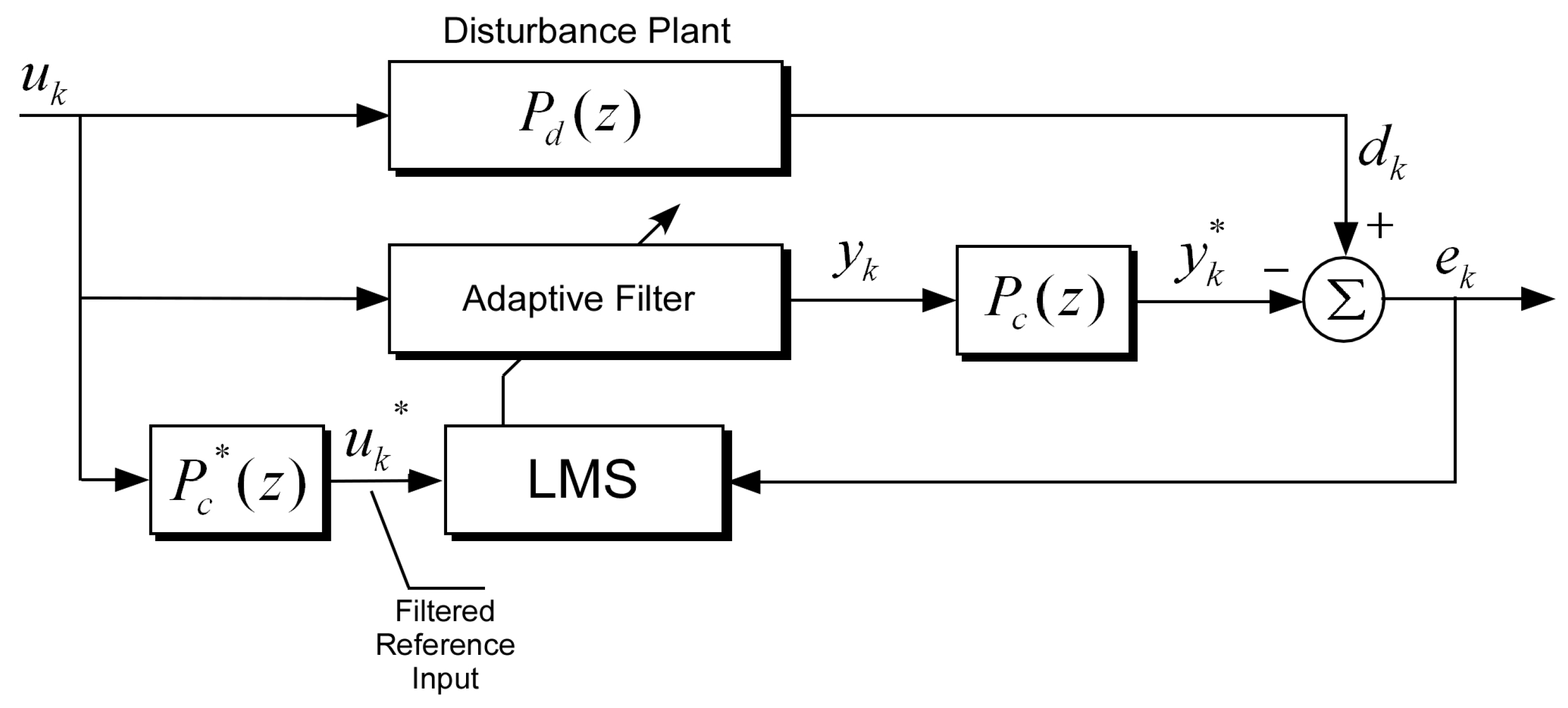
Among a number of adaptive filtering algorithms, the LMS method is the most prevalent feedforward control algorithm because of its relative simplicity [15]. It adjusts a digital filter by the reference input uk, with frequency components to be dealt with; the measured error ek at the current moment; the gap of the adaptive filter output yk and the desired value dk. This algorithm makes the output of the filter close to the plant output, which is the desired signal. Updating the equation for the filter coefficients of the LMS can be acquired with the minimization of the mean squared error chosen by a cost function [16].
Here, wk stands for the weight vector of the filter and μ adjusts the stability and the speed of the process. Figure 1 represents the diagram of a common digital filter system. It can be noticed that the filter coefficients cannot track the actual surface of the steepest descent, since the weight changes are calculated by gradient estimates with simplification assumptions. This factor would induce a rather crude tracking performance.
The LMS algorithm is suitable for cases where there are no dynamics in the secondary path of the control system. Nevertheless, in most practical situations, some influences could exist from the sensors, actuators, amplifiers, filters, digital converters, and so on. The algorithm would not function appropriately with such effects. The most usual type of the secondary path dynamics is a time delay or a phase shift, and the overall system seems to converge to a trivial value or become unstable, because the signal yk* and the filter output yk are distinct.
The FX-LMS is a modification of the above LMS method that incorporates the dynamics of the secondary path, which have been obtained beforehand [17]. This algorithm consists of a filtered reference and it is broadly known that FX-LMS is more stable when the dynamics of the secondary path cannot be ignored. The below equation defines the FX-LMS.
The significant property of the Pc*(z) filter is that its response with impulse contains the identical quantity of time delay with the dynamics of the secondary path Pc(z). However, there are noticeable defects of the FX-LMS, which a system identification (ID) procedure is needed so as to obtain the Pc*(z) offline in advance. An online system ID might be possible also, but it causes the overall control system complex and it is difficult to implement.
3. Internal Model Control
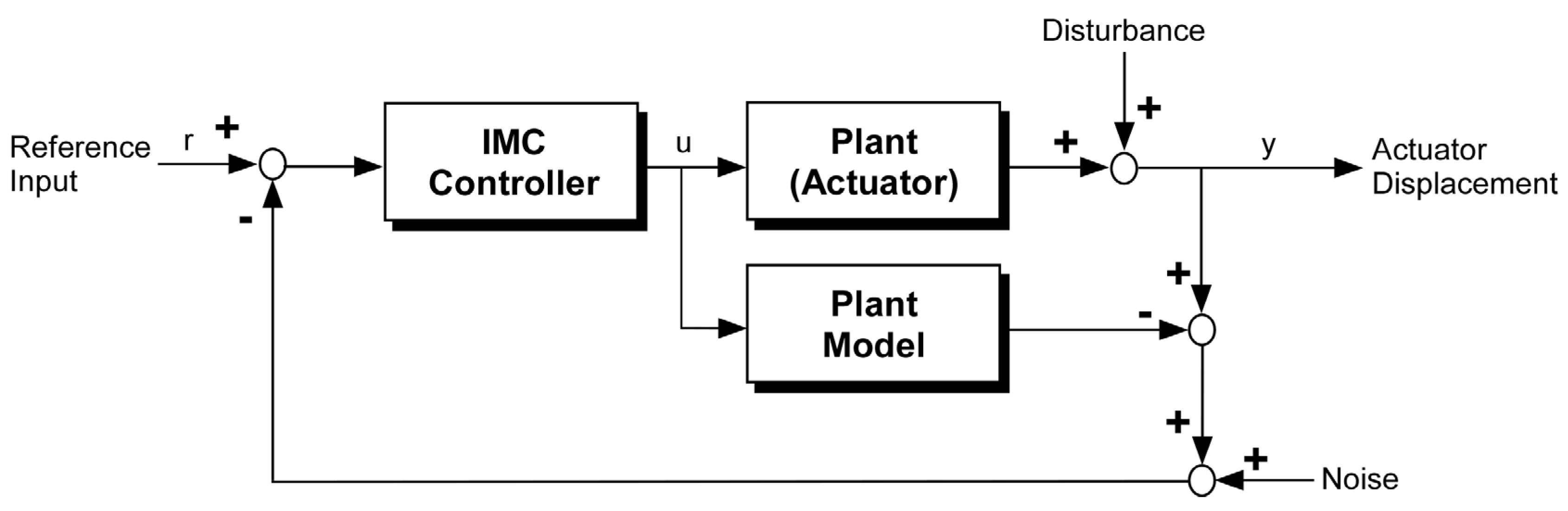
IMC uses the plant model as a component of the controller [18]. The IMC has a number of benefits compared with the traditional PI (proportional-integral) control. First of all, the closed-loop stability is guaranteed merely by selecting a stable controller if an accurate plant model can be obtained. Furthermore, the controller design is relatively straightforward and closed-loop performance properties, such as the rising time, settling time, and time constant, are directly correlated with the control parameters. This makes online tuning of the controller very convenient. The IMC structure is a modification of a classical feedback structure, with the process model applied definitely as an internal part of the controller [19]. The general structure of an IMC system is shown in Figure 2.
The purpose of designing an IMC controller is to force the output to respond to a set point change with desired manners and counter the effects of disturbances. If the controller gain is the inverse of the model gain, and the controller is tuned to assure stability, the process output y will eventually reach and maintain the set point ys in the absence of new disturbances. Unfortunately, a model is never perfect. In addition, if the model has any dynamics at all, rather than just a gain, no controller can perfectly invert the process model. A controller can, however, come very close to inverting the process model. Just how close it can come is the subject of the IMC design problem, in order to expect perfect models. When no zeros are near the imaginary axis or in the right half of the s-plane, the inverse of the model is stable and not overly oscillatory. If the form of the process is defined as Equation (3), where N(s) and D(s) are polynomials of s, the internal model controller can be chosen easily as follows.
In this form, the filter f(s) has two parameters, λ and r. The relative order r is the order of the denominator minus the order of the numerator and it is selected to be large enough for q(s), in order to be proper. The filter time constant λ is selected in order to avoid excessive noise amplification. The main advantage is that closed-loop stability is assured simply by choosing a stable internal model controller. In addition, it has systematic and relatively straightforward design methods, with advantages such as internal stability, stability robustness, and performance robustness. The structure is also intuitive, and the closed-loop performance characteristics are directly related to the controller parameters, making online tuning of the IMC very convenient.
Consider the following model for an arbitrary plant T(s) with second-order linear system dynamics P(s) and time-varying delay term D(s), as follows:
Here, a, ωn, , and τ are the proportional gain, natural frequency, damping ratio, and time delay, respectively. As IMC is a linear controller that requires a linear system model, the exponential function in the model needs to be linearized. For this purpose, (0, 1) the Padé approximation is applied so as to convert the exponential function into a rational function, such that the following, and then the actuator model, becomes linearized, as follows:
With this model, an internal model controller can be designed. By taking the reciprocal of the plant model, the controller transfer function can be written as follows:
where the term (λs + 1)p in the denominator is introduced in order to make the transfer function proper (i.e., the order of the denominator is not lower than that of the numerator). Therefore, p needs to be determined by the order of the numerator in the controller transfer function. In this case, p = 3 is used. The time constant λ in the new term depends on the modeling errors and the allowable noise amplification by the controller. Although IMC uses the plant model in the controller design, good performance cannot be expected unless the exact model of the plant is known. Moreover, if there are discrepancies between the plant model and the actual plant dynamics, IMC can render the controlled system unstable. The main limitation of the IMC stems from the fact that they are basically linear control methodologies, while the plant is nonlinear.
4. Enhanced LMS Methods with IMC
This part discusses the investigation of the two enhanced LMS methods, with a supporting model-based control scheme. The key topic is the use of IMC. Two different structures of adaptive digital filtering systems have been proposed, based on IMC for active noise and vibration attenuation. These systems promote stability performance and enable the multi-spectral control of disturbances in order to manage noise signals and a number of frequency elements in a certain signal simultaneously.
4.1. Novel Adaptive Filtering Algorithm Based on the IMC 1: Non-Recursive Method
4.1.1. Conceptual Explanation
As mentioned, the LMS algorithm could cause instability of the whole control system, or an incorrect solution may be obtained after convergence, since neglecting the secondary path dynamics Pc is essentially unavoidable in realistic situations. The FX-LMS algorithm overcomes this inadequacy by using a reference filter for the input and by compensating for time and phase delays that are induced by several auxiliary parts that are included in the filtering system (sensors, converters, amplifiers, etc.).
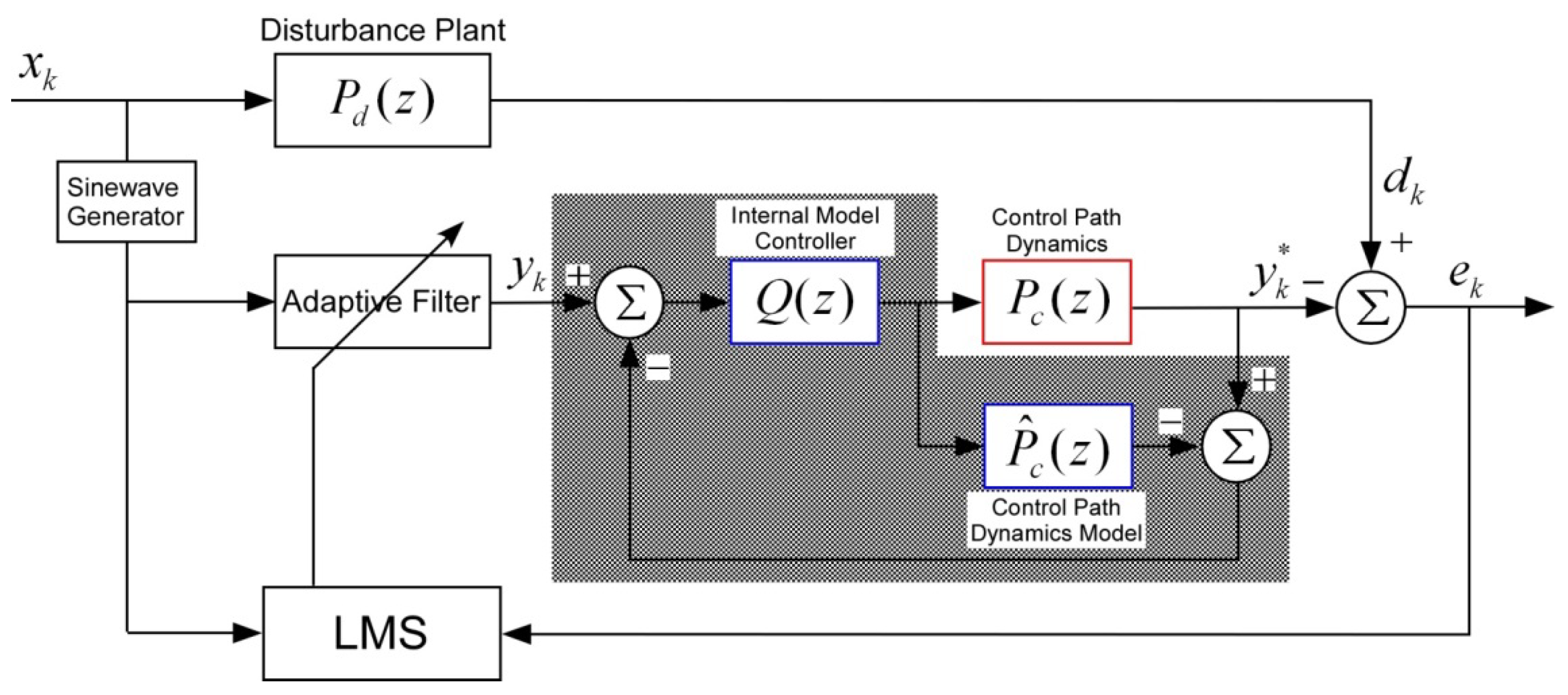
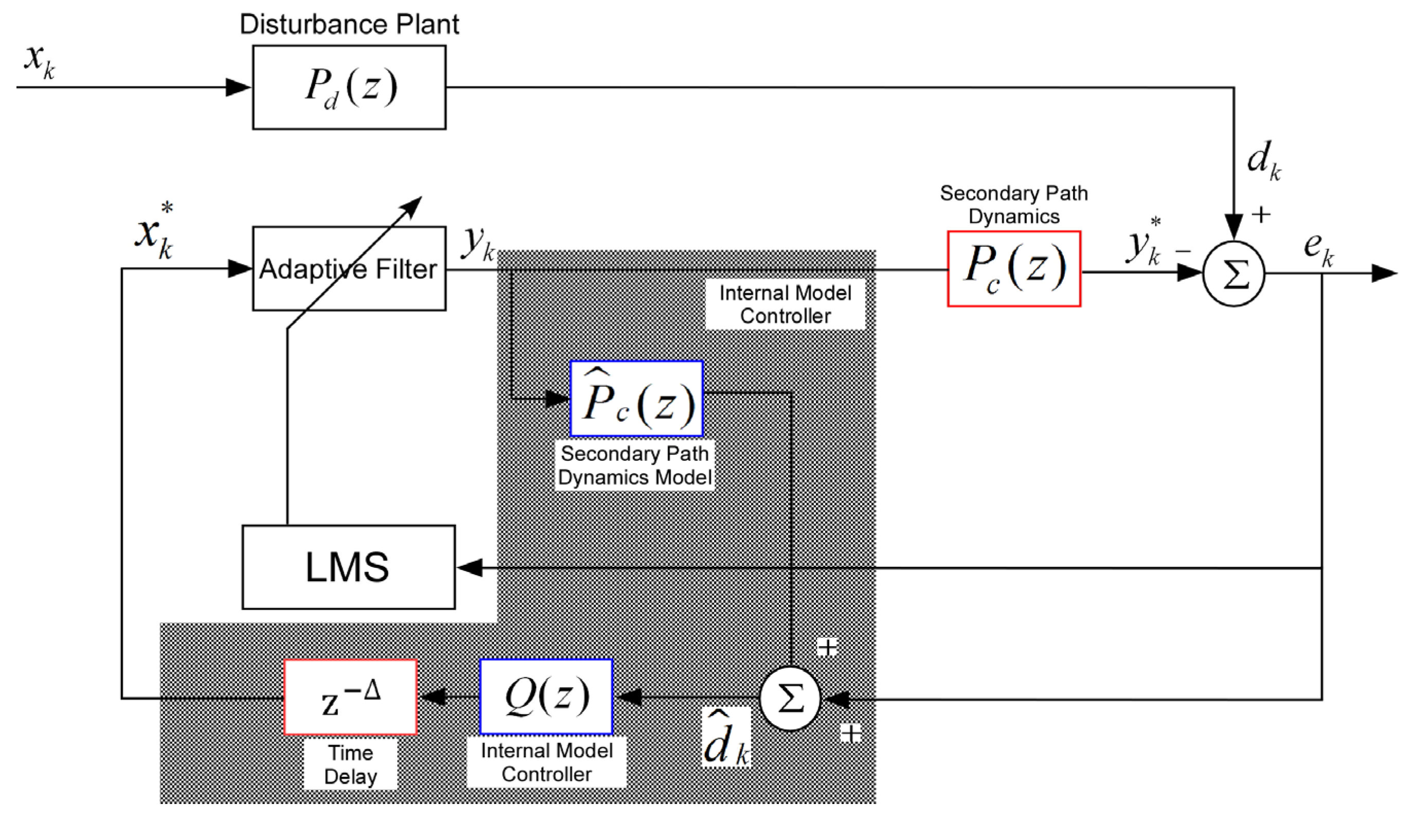
However, the model of the secondary path dynamics must also be identified offline in advance, in order to obtain the coefficients of the filter, which adds to the effort that is needed to implement the control system. Thus, the IMC can be substituted for the filter after the reference signal in the FX-LMS system, as shown in Figure 3. The IMC system is inserted before the secondary path dynamics, so that the effect of Pc can be compensated without destabilizing the adaptive filtering system. If we roughly know the dynamics of the secondary path, there is no need to identify it offline beforehand, and the control system can be implemented immediately. The key point for this novel method is that the filtered-X LMS algorithm is not needed for the system with secondary path dynamics and the offline process for identification is not required if we have ‘even’ a rough model of the secondary path.
The shaded region of Figure 3 indicates the IMC system for the secondary path dynamics Pc. The internal model controller Q is designed based on an estimated model . Let the value right before the internal model controller Q be tk. Then, the following equation holds.
The last two terms on the right-hand side are as follows.
From Equation (10b–d), Equation (9) becomes the following:
By arranging Equation (11) with yk*, the difference between the original filter output yk and the IMC compensated filter output yk* can be obtained as follows.
If an exact model of the secondary path dynamics can be obtained, , and Equation (12) becomes the following:
yk and yk* would be very close to each other after applying the IMC if the value λ can be selected properly, and the system instability that is caused by the secondary path dynamics would be decreased.
4.1.2. Numerical Validation
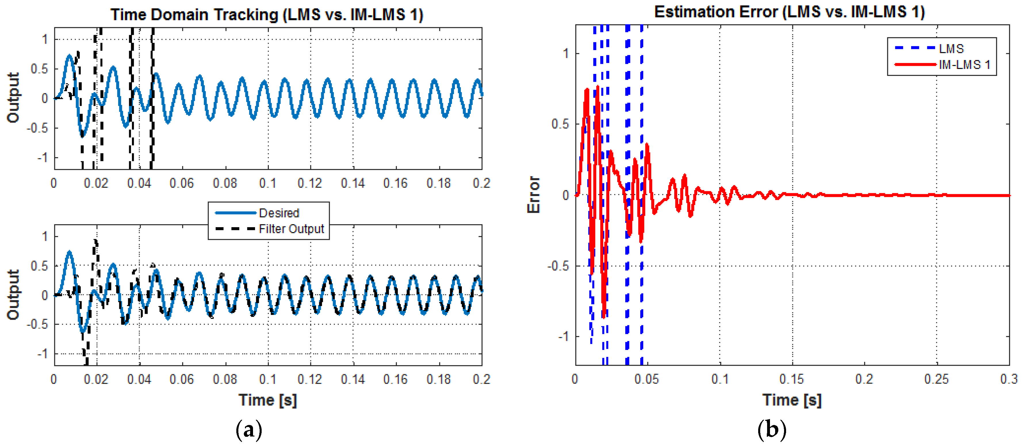
The proposed technique was implemented in numerical simulations and was validated by comparison with the conventional LMS algorithm. An adaptive digital filter with a FIR filter structure has been defined with two coefficients. The target disturbance plant is assumed to be a second order system with a natural frequency of ωn = 50 Hz and a damping ratio of = 0.1. A sinusoidal input signal x(t) = A1sin(ω1t + θ1) with one frequency component at ω1/2π = 100 Hz is used as both the input reference and the disturbance plant input (A1 = 1, θ1 = 0). The μ value was chosen as 0.4 for both cases.
In the first case, suppose that the input filter is not used in an adaptive filtering system when the secondary path dynamics Ps(z) cannot be neglected. The secondary path is presumed to be a first-order system, with a time constant 0.01, as in Equation (14b), and the exact model is assumed to be available. The internal model controller Q(z) can be designed as Equation (14c), with the model of the target plant following the procedure in Section 3. The value of λ is chosen as 0.002.
Figure 4a compares the time domain tracking of the desired signal with a sinusoidal input under the control of the LMS and the internal model LMS method 1 (IM-LMS 1). Figure 4b shows the estimation error. The conventional system with LMS becomes unstable and diverges without the filtered reference signal, but IM-LMS 1 can manage this condition just as with the filtered-X LMS system, and the whole system can follow the reference signal with stability.
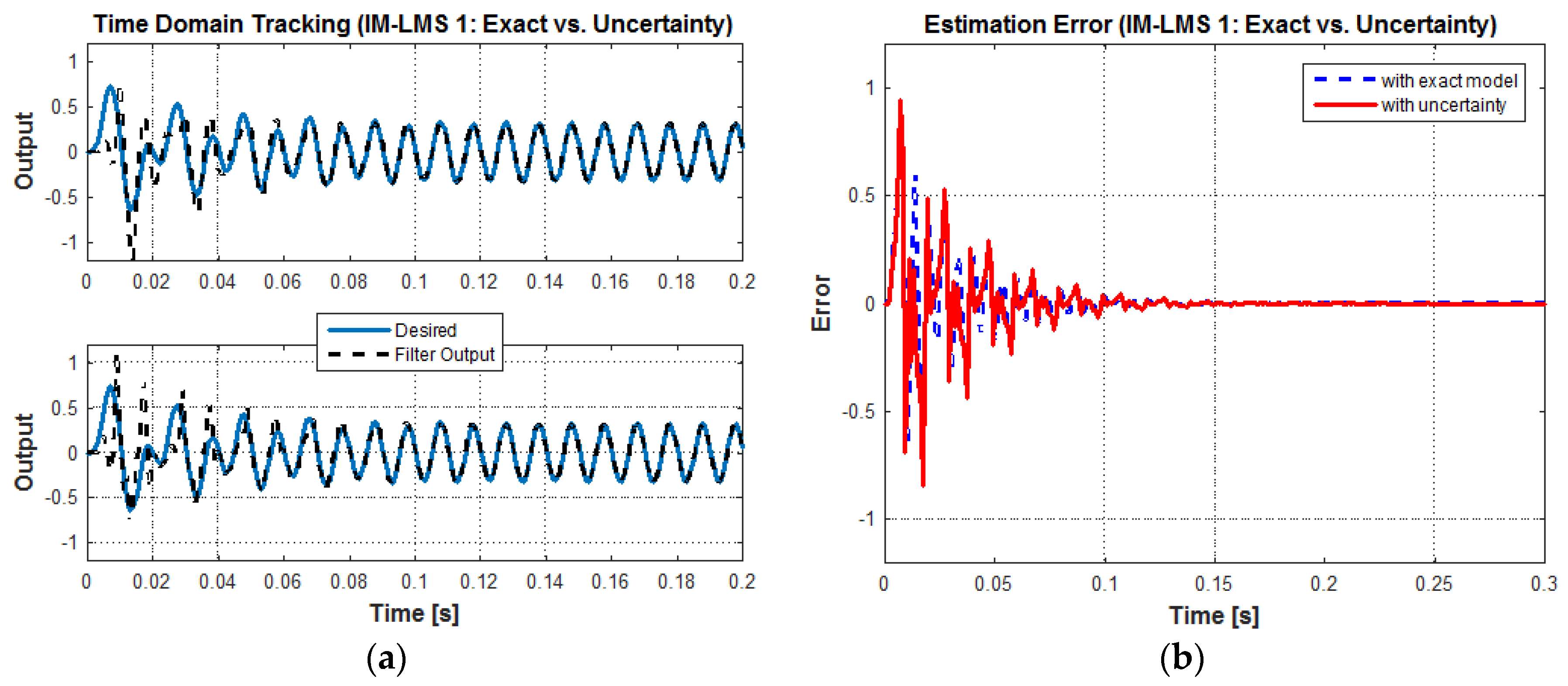
Assuming the same conditions as the previous case, Figure 5a compares the time-domain tracking of the desired signal under the control of IM-LMS 1, with an exact model and with uncertainty. Figure 5b shows the estimation error. In the transient state, up to around 0.1 s, uncertainty in the model induces more error than the exact model. However, after that point, the error converges to zero in the steady state. Although a significantly mistuned plant model has been used in the control system, the IM-LMS 1 method made the system converge and showed an acceptable tracking performance. This suggests that the new algorithm has more self-adaptability.
Next, to check the tracking performance of the algorithm, the IM-LMS 1 algorithm was evaluated for the amplitude-modulated (AM) signal xa(t), which is defined as follows:
xa(t) contains a sinusoid at ωoa/2π = 12 Hz, which is modulated with a carrier signal at ωca/2π = 150 Hz and has a modulation depth of B0a = 0.5. For convenience, A0a is normalized as 1.0, and the phase angles θc and θo are ignored. A sinusoid at ωca is used as a reference input. Equation (16b), F[ ] illustrates the Fourier transform, and δ indicates the Dirac delta function that is located at frequency ω. The LMS parameter μ is chosen as 0.5. For comparison, the same signal is also tracked by the conventional FX-LMS.
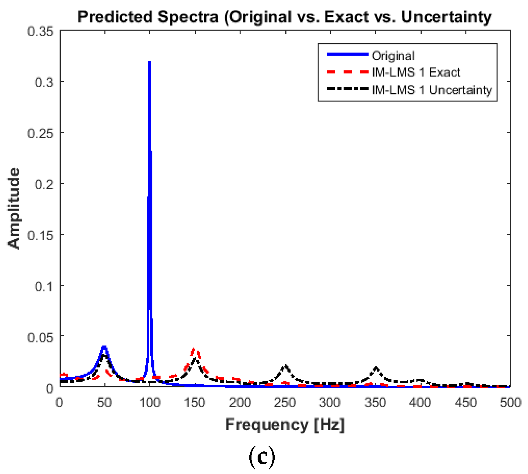
Figure 6a compares the time domain tracking of the desired signal with the filter output, for both FX-LMS and IM-LMS 1. Although IM-LMS 1 works, as well as the FX-LMS, with no need for a filtered reference, it has a much worse tracking performance. The estimation error of IM-LMS 1 shown in Figure 6b even grows over time. This indicates that IM-LMS 1 is merely helping the LMS method to accomplish a more stabilized control system and is not suitable for controlling multi-spectral signals.
4.2. Novel Adaptive Filtering Algorithm Based on the IMC 2: Recursive Method
4.2.1. Conceptual Explanation
IM-LMS 1 showed a better stability performance than the conventional LMS algorithm without filtered reference input signals, and no offline tuning of the secondary path dynamics was needed, which makes the proposed method convenient. However, the tracking performance of this adaptive filtering system is at the same level as the established method, so more efforts with a modified algorithm and system structures are needed. Mechanical systems that generate noise and vibration, such as vehicles, engineering structures, and electromechanical systems, have become more complicated, and the signals contain very rich frequency spectra. The selection of a reference input is important as it determines the tracking performance. An alternative technique based on IMC is thus needed to effectively deal with signals that have a complex frequency spectra.
Consequently, a recursive loop is proposed into the digital filter system. The schematic of the IMC-based adaptive digital filtering system with a ‘recursive’ LMS algorithm is shown in Figure 7.
The fundamental concept of this system is to create or estimate a reference signal xk* for the LMS algorithm in real time, with an estimated output of the disturbance plant . The error signal ek is the difference between the output of the disturbance plant dk and the output of the secondary path dynamics yk*. The estimated output of can be obtained by adding ek to the filtered output signal with the internal model of the secondary path dynamics Pc. Here, k indicates the sampling instant, and a time delay block z−Δ is placed as a result of the estimation process and the secondary path dynamics. In order to minimize the effect of this type of time delay, the internal model controller is again introduced and it is designed based on the secondary path dynamics . It is basically a single-channel system with one reference signal and one error sensor, and it can be extended to cover multi-channel signals.
The filtered output signal yf_k is defined by multiplying yk with an internal model , which estimates the impulse response of the secondary path dynamics:
The estimated reference signal xk* in the recursive adaptive filtering system can then be obtained.
The output signal yk of the adaptive filter wk is calculated using Equation (20), where wk is the weight vector of the filter and L is the length of the adaptive filter.
The weight update algorithm is the same as the conventional digital filter system with the LMS. The adaptive weight vector wk is updated with the following equation:
where μ is the step size. The error signal ek is obtained, and the output of the filter that has been affected by the secondary path dynamics yk* is defined as follows:
The traditional feedback ANC system with the filtered-X LMS algorithm has filter before the reference signal. However, in this novel system, internal model control is introduced and it is used for compensating unavoidable time delay in the feedback loop. This kind of time delay is actually from the secondary path dynamics and the estimation process. At least, the effect from the secondary path dynamics can be managed and it does not need offline identification process for the secondary path again.
4.2.2. Numerical Validation
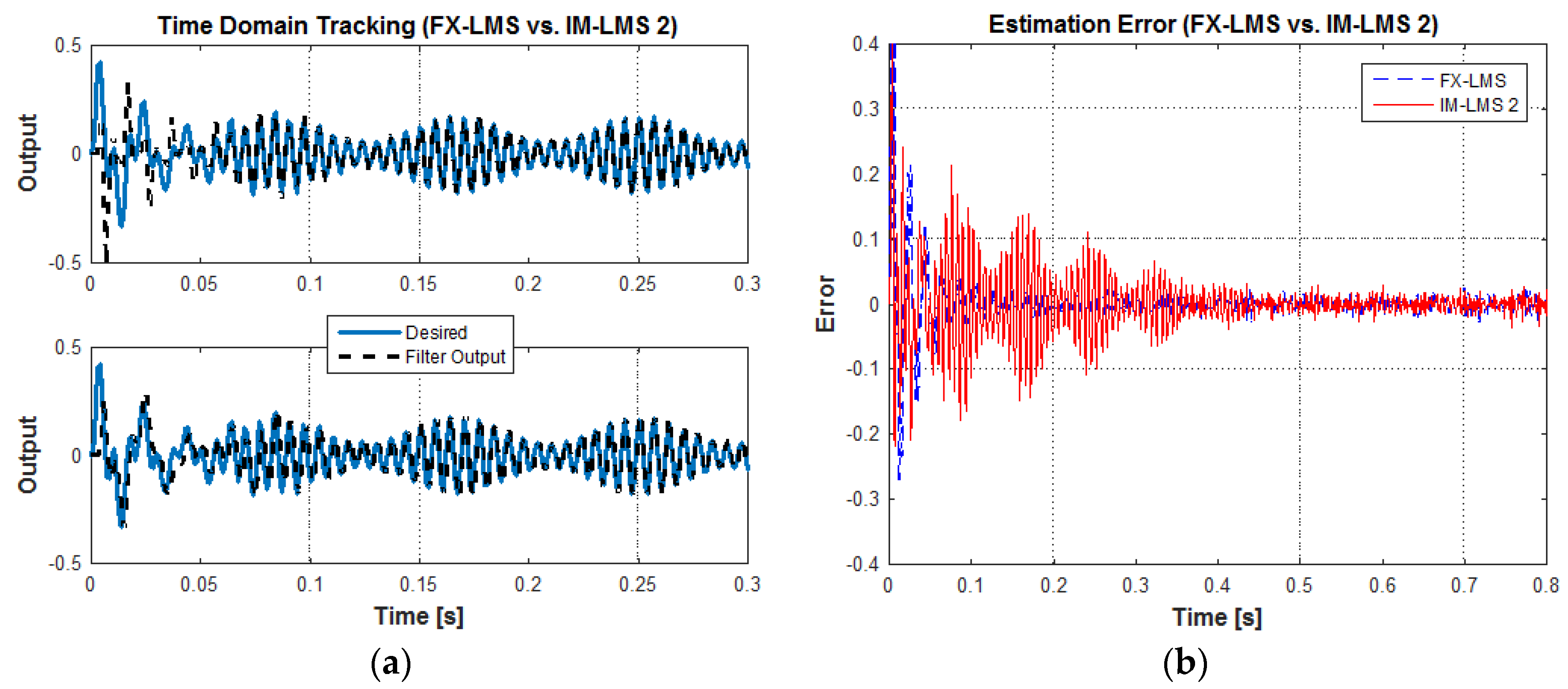
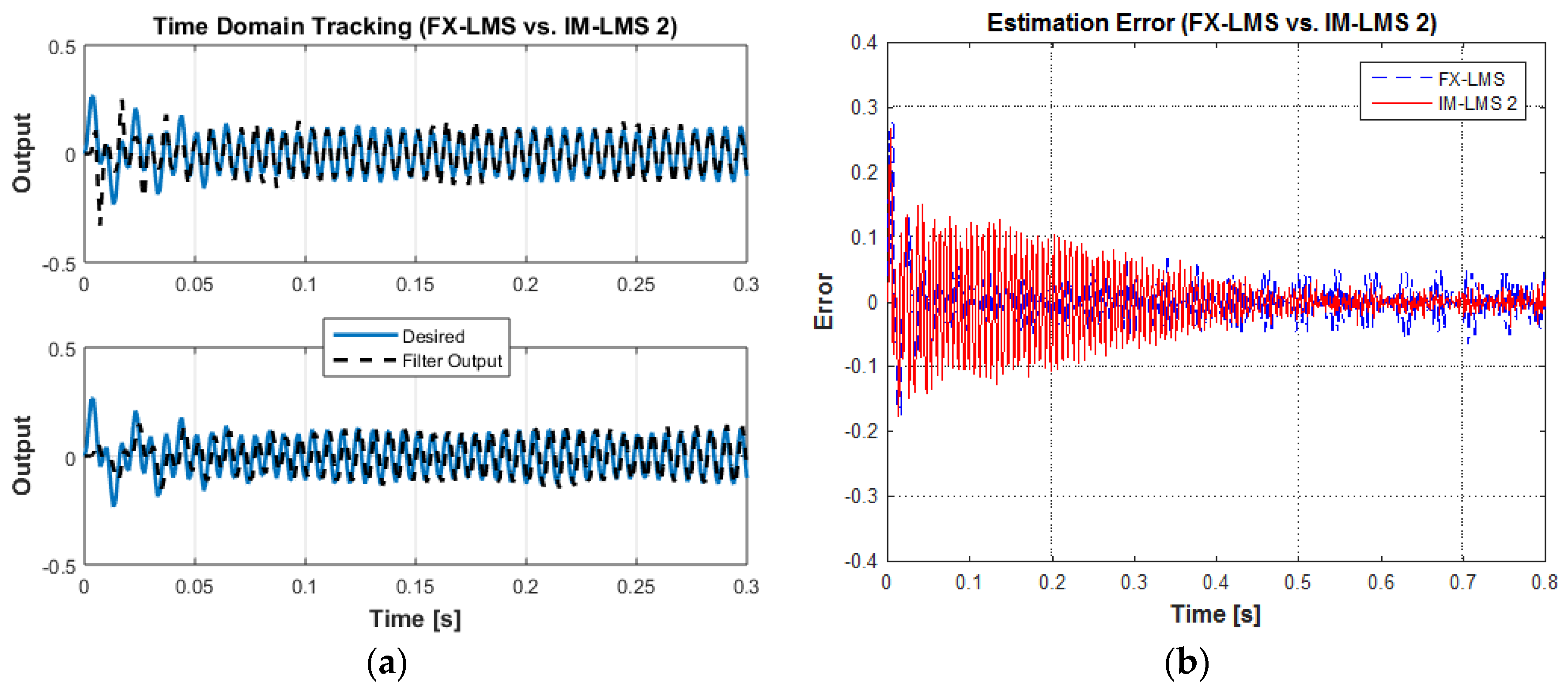
The internal model LMS method 2 (IM-LMS 2) was validated for two different kinds of multi-spectral signals, namely, AM and frequency-modulated (FM) signals. The same AM signal is used for evaluating the method. Figure 8 compares the tracking performance and estimation error of the conventional LMS and IM-LMS 2. In the transient region, up to around 0.05 s, the IM-LMS 2 method shows a much better tracking performance, as shown in Figure 8a. However, in the steady-state region after 0.05 s, the IM-LMS 2 has a slower convergence than FX-LMS, for around 0.4 s (0.05 ≤ t ≤ 0.45), and finally, the estimation errors of both of the methods have similar peak-to-peak values, as shown in Figure 8b.
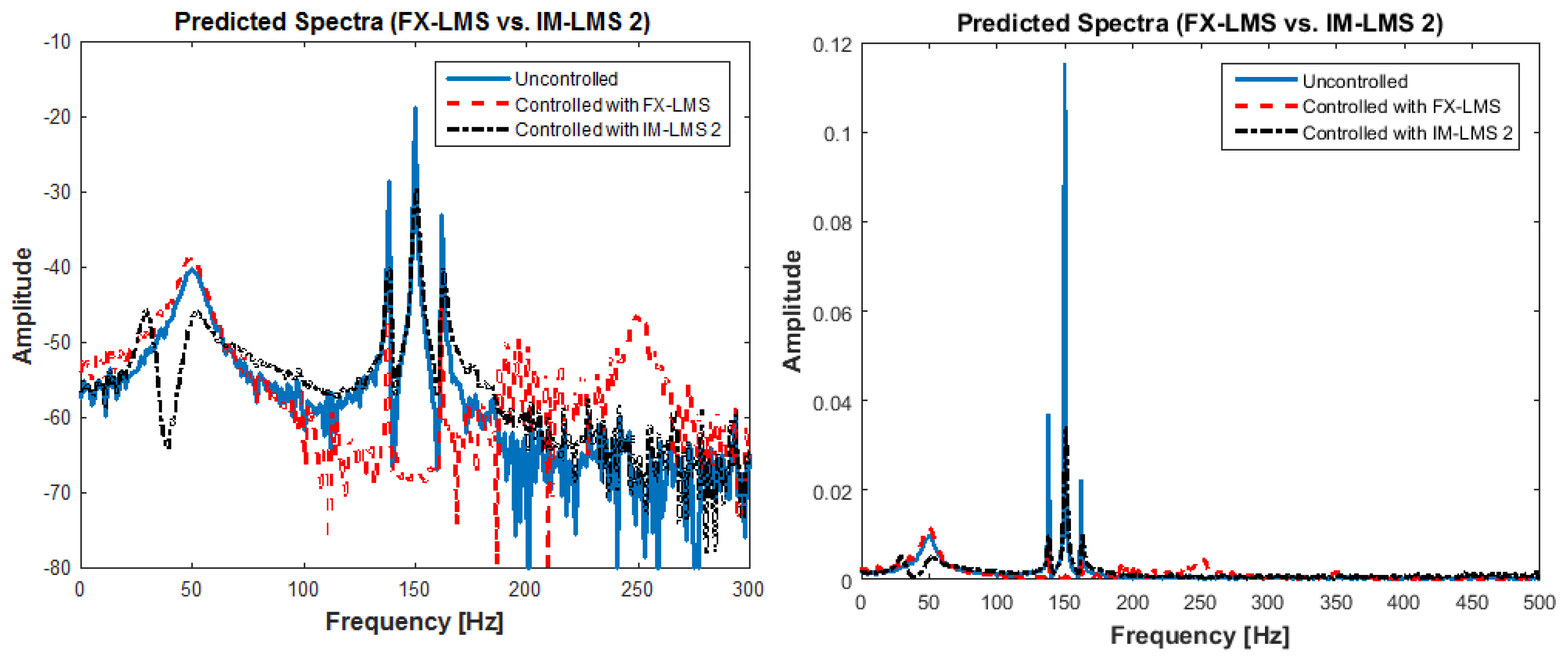
Since FX-LMS is targeted only to the 150 Hz frequency component ωca, the time-domain tracking in steady state would have been superior to that of IM-LMS 2. This is clear in the frequency spectrum plot of Figure 9, which shows a difference of in magnitude of almost 30 dB at 150 Hz. This figure compares the predicted spectra of the uncontrolled AM signal and controlled AM signal with both of the methods. Although a broadband reduction cannot be achieved with either FX-LMS or IM-LMS 2, they have shown significant reductions at primary peaks (ωca, ωca − ωoa, ωca + ωoa). The amplitude reduction levels of FX-LMS at the primary peaks are higher than those of IM-LMS 2, while FX-LMS shows a severe spillover at higher frequency, from around 180 Hz to 270 Hz. This indicates that the conventional LMS algorithm with a feedforward control structure is insufficient to control the multi-spectral signals, without full knowledge of the original signal.
In addition, the IM-LMS 2 method shows considerable attenuation at around 50 Hz, which is the natural frequency of the target plant, whereas the FX-LMS case demonstrates similar amplitude levels around this frequency. This condition comes from the benefit of the recursive structure of the adaptive control system, where untargeted peaks could be directly handled by feeding the estimated plant output back to the reference input of the LMS algorithm. Therefore, the whole control system identifies the frequency components other than ωca. In contrast, the conventional FX-LMS still recognizes only the ωca component of x(t). Overall, IM-LMS 2 uses recursive control techniques and exploits both the conventional LMS algorithm and IMC simultaneously. However, there is some trade-off in the tracking performance with the conventional FX-LMS.
The FM signal was investigated similarly, as shown in Equation (25a,b).
Jn indicates a Bessel function of order n, and the modulation depths A0f, B0f, and θf are selected as 1.0, 0.5, and 0, respectively. The reference input and other parameters that were used are the same as those for the AM case.
Figure 10 compares the tracking performance and estimation error of the conventional LMS and IM-LMS 2 methods. Similar trends to the AM signal case are observed for up to 0.45 s. In the transient region, for up to around 0.05 s, the IM-LMS 2 method shows a much better tracking performance but a slower convergence than the FX-LMS, for around 0.4 s (0.05 ≤ t ≤ 0.45) in the steady-state region. However, after that point, the peak-to-peak value of the estimation error with the IM-LMS 2 is about three times better than that of FX-LMS.
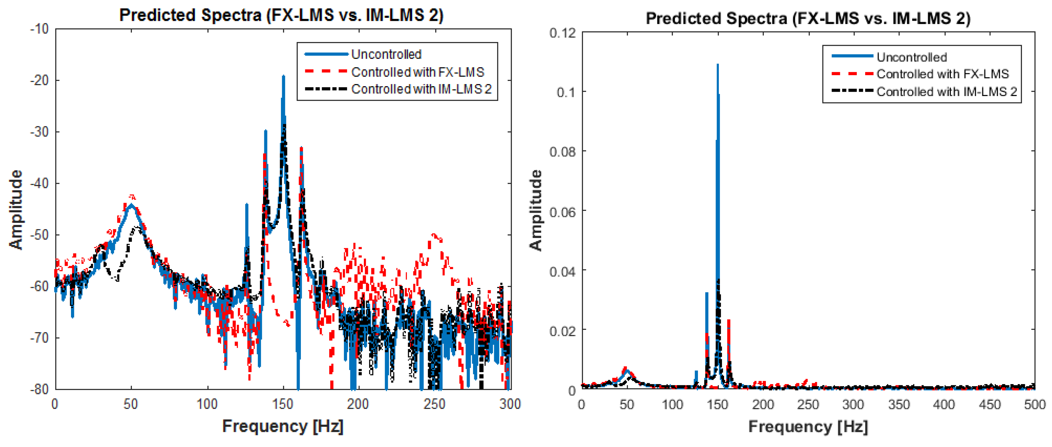
Figure 11 compares the predicted spectral contents of the uncontrolled FM signal and controlled FM signal for both of the methods. Although a broadband reduction cannot be achieved with either FX-LMS or IM-LMS 2, they show significant reductions at primary peaks (ωcf, ωcf − nωof, ωcf + nωof). The amplitude reduction levels of IM-LMS 2 at primary peaks are higher than those of FX-LMS, except for at ωcf, while FX-LMS shows a severe spillover at a higher frequency. In addition, the IM-LMS 2 method shows considerable attenuation at around 50 Hz, which is the natural frequency of the target plant, whereas FX-LMS demonstrates similar amplitude levels around this frequency. Thus, the tracking performance of IM-LMS 2 is improved when increasing the complexity and frequency components that were to be controlled in the output of the disturbance plant, which should be tracked.
5. Conclusions and Future Work
Two enhanced LMS methods were introduced for an adaptive digital filtering system combined with IMC, in order to take advantage of having the process model inside the control system structure.
Major contributions of this research comprise the following. Firstly, the internal model LMS method 1 (IM-LMS 1) is introduced, which is a novel model-based algorithm. Internal mode control is applied in the traditional LMS algorithm, for assuring convergence of the control system without filtered inputs. It also showed acceptable tracking performance with a significantly mistuned plant model. Secondly, the internal model LMS method 2 (IM-LMS 2) is proposed. A new recursive digital filter system is proposed with an internal model controller. This control system enhances robustness, stability, and the ability to manage multi-spectral signals. Moreover, the tracking performance of IM-LMS 2 is improved with increasing complexity and frequency components to be controlled in the output of the disturbance plant, which should be tracked. Thirdly, with numerical analyses, their performances are validated. Proposed algorithms are numerically verified in several cases with single sine waves and multi-spectral signals. Time domain tracking performances and estimation errors in time and frequency domains are compared and their characteristics are discussed.
This research will be verified with large number of applications for active noise and vibration control, including vibration mitigation, vehicle noise, and vibration attenuation. This research could be used to improve the active control applications in vehicles and mechanical structures with effective management of an expansive range of multi-spectral signals.
Author Contributions
B.K. and J.-Y.Y. initiated and developed the ideas related to this research work; B.K. and J.-Y.Y. developed novel methods, derived relevant formulations, and carried out performance analyses and numerical analyses; B.K. wrote the paper draft under J.-Y.Y.’s guidance; and B.K. finalized the paper.
Acknowledgments
This work was supported by the 2016 Yeungnam University Research Grant (216A580005).
Conflicts of Interest
The authors declare no conflict of interest.
Nomenclature
| D(s) | time-varying delay |
| D(s) | denominator |
| F[ ] | Fourier transform |
| Jn | Bessel function of order n |
| L | length of filter |
| N(s) | polynomials of numerator |
| Pc(z) | secondary path dynamics |
| T(s) | arbitrary plant |
| Q | internal model controller |
| a | proportional gain |
| dk | desired value |
| ek | measured error |
| k | sampling instant |
| p(s) | process model |
| q(s) | internal model controller |
| r | relative order |
| uk | reference input |
| wk | weight vector of filter |
| z−Δ | time delay block |
| xa(t) | amplitude-modulated |
| xf(t) | frequency-modulated |
| yk | adaptive filter output |
| ys | set point |
| δ | Dirac delta function |
| ξ | damping ratio |
| λ | filter time constant |
| μ | convergence factor |
| τ | time delay |
| ωn | natural frequency |
| ^ | parameters of FX LMS |
| * | after secondary path |
References
- Bai, M.; Luo, W. DSP implementation of an active bearing mount for rotors using hybrid control. ASME J. Vib. Acoust. 2000, 122, 420–428. [Google Scholar] [CrossRef]
- Adeli, H.; Kim, H. Hybrid feedback-least mean square algorithm for structural control. J. Struct. Eng. 2004, 130, 120–127. [Google Scholar] [CrossRef]
- Bouchard, M.; Paillard, B. An alternative feedback structure for the adaptive active control of periodic and time-varying periodic disturbances. J. Sound Vib. 1998, 210, 517–527. [Google Scholar] [CrossRef]
- Pan, M.; Wei, W. Adaptive focusing control of DVD drives in vehicle systems. J. Vib. Control 2006, 12, 1239–1250. [Google Scholar] [CrossRef]
- Sabah, Y.; Okuma, M.; Okubo, M. Implementation of single and multiple adaptive step-size algorithm to ANC. ASME J. Vib. Acoust. 2007, 130, 014503. [Google Scholar] [CrossRef]
- Hao, L.; Li, Z. Modeling and adaptive inverse control of hysteresis and creep in ionic polymer-metal composite actuators. Smart Mater. Struct. 2010, 19, 025014. [Google Scholar] [CrossRef]
- Carnahan, J.; Richards, C. A modification to filtered-X LMS control for airfoil vibration and flutter suppression. J. Vib. Control 2008, 14, 831–848. [Google Scholar] [CrossRef]
- Akhtar, M.; Mitsuhashi, W. Improving performance of FxLMS algorithm for active noise control of impulsive noise. J. Sound Vib. 2009, 327, 647–656. [Google Scholar] [CrossRef]
- Zhang, Z.; Hu, F.; Wang, J. On saturation suppression in adaptive vibration control. J. Sound Vib. 2010, 329, 1209–1214. [Google Scholar] [CrossRef]
- Kuo, S.; Gupta, A.; Mallu, S. Development of adaptive algorithm for active sound quality control. J. Sound Vib. 2007, 299, 12–21. [Google Scholar] [CrossRef]
- Zhou, D.; Li, J.; Hansen, C. Application of least mean square algorithm to suppression of maglev track induced self-excited vibration. J. Sound Vib. 2011, 330, 5791–5811. [Google Scholar] [CrossRef]
- Wang, T.; Gan, W. Stochastic analysis of FXLMS-based internal model control feedback active noise control systems. Signal Process. 2014, 101, 121–133. [Google Scholar] [CrossRef]
- Shafiq, M.; Riyaz, S. Internal model control structure using adaptive inverse control strategy. In Proceedings of the Fourth International Conference on Control and Automation (ICCA’03), Montreal, QC, Canada, 12 June 2003; pp. 148–152. [Google Scholar]
- Zhu, H.; Liu, J.; Chang, T.; Tian, L. Internal Model Control Using LMS Filter and Its Application to Superheated Steam Temperature of Power Plant. In Proceedings of the 2nd International Conference on Computer and Automation Engineering (ICCAE), Singapore, 26–28 February 2010; pp. 135–138. [Google Scholar]
- Kuo, S.; Morgan, D. Active Noise Control Systems: Algorithms and DSP Implementations; John Wiley & Sons: Hoboken, NJ, USA, 1996. [Google Scholar]
- Widrow, B.; Stearns, S. Adaptive Signal Processing; Prentice-Hall: Upper Saddle River, NJ, USA, 1985. [Google Scholar]
- Widrow, B.; Glover, J.; McCool, J.; Kaunitz, J.; Williams, C.; Hearn, R.; Zeidler, J.; Dong, E.; Goodlin, R. Adaptive noise cancelling: Principles and applications. Proc. IEEE 1975, 63, 1692–1716. [Google Scholar] [CrossRef]
- Garcia, C.; Morari, M. Internal Model Control. 1. A Unifying Review and Some New Results. ACS Ind. Eng. Chem. Process Des. Dev. 1982, 21, 308–323. [Google Scholar] [CrossRef]
- Brosilow, C.; Joseph, B. Techniques of Model-Based Control; Prentice Hall PTR: Upper Saddle River, NJ, USA, 1999. [Google Scholar]
Figure 1.
Digital filtering system with filtered-X least mean square (FX-LMS) algorithm.

Figure 2.
Internal model control (IMC) system.

Figure 3.
Schematic of a new digital filtering system with LMS, based on the internal model control (IM-LMS 1).
Figure 3.
Schematic of a new digital filtering system with LMS, based on the internal model control (IM-LMS 1).

Figure 4.
Simulation results in time domain with a single sinusoid at 100 Hz. (a) Time domain tracking with LMS and internal model LMS 1 methods; (b) estimation error; (c) predicted spectra.
Figure 4.
Simulation results in time domain with a single sinusoid at 100 Hz. (a) Time domain tracking with LMS and internal model LMS 1 methods; (b) estimation error; (c) predicted spectra.


Figure 5.
Simulation results in the time domain (single sinusoid at 100 Hz) with LMS and internal model LMS 1 methods. (a) With exact model (top) and with uncertainty (bottom); (b) comparison of estimation error; (c) predicted spectra.
Figure 5.
Simulation results in the time domain (single sinusoid at 100 Hz) with LMS and internal model LMS 1 methods. (a) With exact model (top) and with uncertainty (bottom); (b) comparison of estimation error; (c) predicted spectra.


Figure 6.
Control of an amplitude-modulated (AM) signal. (a) Time-domain tracking with LMS and internal model LMS 1 methods; (b) estimation error; (c) predicted spectra.
Figure 6.
Control of an amplitude-modulated (AM) signal. (a) Time-domain tracking with LMS and internal model LMS 1 methods; (b) estimation error; (c) predicted spectra.

Figure 7.
Schematic of a novel digital filter system with ‘recursive’ LMS algorithm, based on internal model control (IM-LMS 2).
Figure 7.
Schematic of a novel digital filter system with ‘recursive’ LMS algorithm, based on internal model control (IM-LMS 2).

Figure 8.
Control of an amplitude-modulated (AM) signal. (a) Time-domain tracking with LMS and internal model LMS 2 methods; (b) estimation error.
Figure 8.
Control of an amplitude-modulated (AM) signal. (a) Time-domain tracking with LMS and internal model LMS 2 methods; (b) estimation error.

Figure 9.
Predicted spectra for an amplitude-modulated (AM) signal with LMS and internal model LMS 2 methods.
Figure 9.
Predicted spectra for an amplitude-modulated (AM) signal with LMS and internal model LMS 2 methods.

Figure 10.
Control of a frequency-modulated (FM) signal. (a) Time-domain tracking with LMS and internal model LMS 2 methods; (b) estimation error.
Figure 10.
Control of a frequency-modulated (FM) signal. (a) Time-domain tracking with LMS and internal model LMS 2 methods; (b) estimation error.

Figure 11.
Predicted spectra for a frequency-modulated (FM) signal with least mean squares and internal model least mean squares 2 methods.
Figure 11.
Predicted spectra for a frequency-modulated (FM) signal with least mean squares and internal model least mean squares 2 methods.

© 2018 by the authors. Licensee MDPI, Basel, Switzerland. This article is an open access article distributed under the terms and conditions of the Creative Commons Attribution (CC BY) license (http://creativecommons.org/licenses/by/4.0/).
Share and Cite
MDPI and ACS Style
Kim, B.; Yoon, J.-Y. Modified LMS Strategies Using Internal Model Control for Active Noise and Vibration Control Systems. Appl. Sci. 2018, 8, 1007. https://doi.org/10.3390/app8061007
AMA Style
Kim B, Yoon J-Y. Modified LMS Strategies Using Internal Model Control for Active Noise and Vibration Control Systems. Applied Sciences. 2018; 8(6):1007. https://doi.org/10.3390/app8061007
Chicago/Turabian StyleKim, Byeongil, and Jong-Yun Yoon. 2018. "Modified LMS Strategies Using Internal Model Control for Active Noise and Vibration Control Systems" Applied Sciences 8, no. 6: 1007. https://doi.org/10.3390/app8061007
Note that from the first issue of 2016, this journal uses article numbers instead of page numbers. See further details here.