Modeling and Control of Negative-Buoyancy Tri-Tilt-Rotor Autonomous Underwater Vehicles Based on Immersion and Invariance Methodology

Abstract

Spot hover and high speed capabilities of underwater vehicles are essential for ocean exploring, however, few vehicles have these two features. Moreover, the motion of underwater vehicles is prone to be affected by the unknown hydrodynamics. This paper presents a novel negative-buoyancy autonomous underwater vehicle equipped with tri-tilt-rotor to obtain these two features. A detailed mathematical model is derived, which is then decoupled to altitude and attitude subsystems. For controlling the underwater vehicle, an attitude error model is designed for the attitude subsystem, and an adaptive nonlinear controller is proposed for the attitude error model based on immersion and invariance methodology. To demonstrate the effectiveness of the proposed controller, a three degrees of freedom (DOF) testbed is developed, and the performance of the controller is validated through a real-time experiment.

1. Introduction

With the increasing demand for marine equipment over the past decades, different types of marine vehicles have been developed to expand human exploration capabilities [1] from the surface to the bottom of the ocean. Underwater vehicles perform various missions, such as collecting samples [2], acquiring data [3], and repairing marine structures [4].

In accordance with the level of autonomy for self-driving vehicles, underwater vehicles can be classified into remotely operated underwater vehicles (ROV) [5], autonomous underwater vehicles (AUV) [6,7], and human occupied vehicles (HOV) [8]. ROV consist of a cable that is used for power supply and as a communication line, which is used by the operator to remotely control the ROV [2,9]; an AUV is autonomous, and it performs motion control and mission planning [10,11,12]; an HOV has a life support system, and a pilot inside the vehicle controls the movement of the HOV for precise movement. ROV and AUV are unmanned underwater vehicles, and therefore, they have the advantages of no risk to life and long operation time. However, the densities of these vehicles are similar to that of the water owing to the buoyancy of the material used [13,14]. This increases the size and drag force, which considerably slows down the speed of the vehicle [15]. In some scenarios, a high-speed underwater vehicle is required to perform time-sensitive missions. Moreover, with the development of deep sea mining [16], a spot hover is a necessary capability for missions such as recharging and payload transition.

Traditional underwater vehicles have a cylindrical shape or an open frame. Cylindrical-shaped underwater vehicles have the advantage of a low drag force. They are propelled using fixed thrusters, and some of these vehicles are equipped with vertical and horizon thrusters to provide extra control forces. An ocean glider is an autonomous underwater vehicle used for ocean science [15,17]; it uses a small change of buoyancy in order to ascend and descend. A fixed wing converts the vertical motion to horizontal motion [18], thus acting like a saw tooth pattern [19]. The energy effect is so high that the glider can continually glide over hundreds of kilometers for months. Open frame vehicles such as an ROV can operate at one spot with the help of multiple rotors [20]; the AUV cannot achieve this [21]. However, the cable connecting the ROV to the mother ship limits the work range of the ROV [2]. A kind of negative buoyancy vehicle is designed to achieve high speed and long cruise range, it is more efficient than traditional AUV at high speed. However, it has to fly in the water to maintain depth, besides, spot hover capability is not achieved [22].

The design and control of an underwater vehicle involves many problems such as the nonlinearity of the model [13,21,23], underactuation [24], and the influence of the ocean current, waves, and turbulence [25].

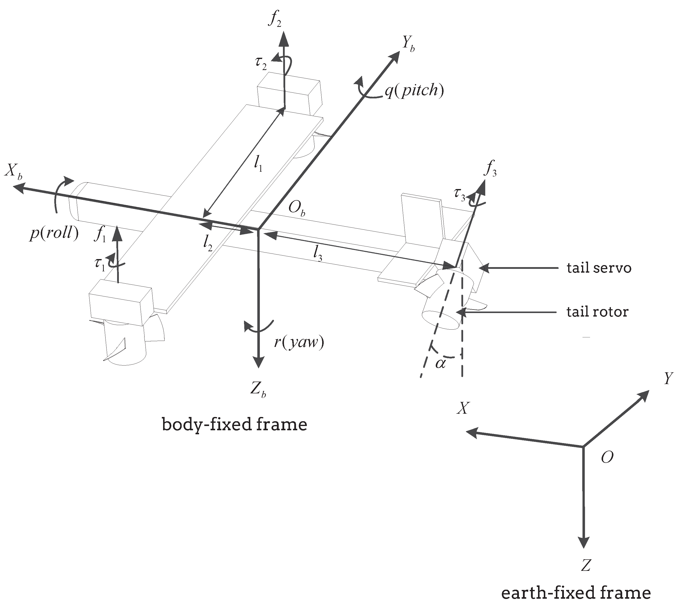
In this paper, we present a negative-buoyancy tri-tilt-rotor autonomous underwater vehicle (NTAUV) to achieve the capability of spot hover and high-speed motion. The NTAUV is illustrated in Figure 1. The NTAUV is heavier than water, has negative buoyancy, and it balances the weight by buoyancy and lift force generated by the fixed wing or thrusters. Further, it operates under three modes: hover, horizontal motion, and transition between them. The NTAUV can hover or slowly cruise by controlling the rotor speed and the tail rotor angle in the hover mode. The hover motion control of NTAUV uses a hierarchical control scheme. The outer layer is position control, and the inner layer is attitude control. Attitude control is the fundamental function of the underactuated system. This paper focuses on hover mode modeling and control, especially attitude control. We design an adaptive nonlinear attitude controller using the immersion and invariance (I&I) methodology.

The article is structured as follows. Section 2 introduces some preliminaries, including the kinematic equations, mechanical structure, mathematical model, and subsystems of altitude and attitude. Section 3.1 presents the attitude error model. In Section 3.2, an adaptive nonlinear I&I controller is designed for the attitude subsystem. The stability analysis is presented in Section 3.3. A three degree of freedom testbed is designed and the experiment results are shown in Section 4.

2. Preliminaries

2.1. Kinematics and Kinetics

Modeling a marine vehicle involves the study of statics and dynamics. The 6 DOF motion of a marine vehicle is analyzed by defining two coordinate frames, as illustrated in Figure 1. $O_b{X}_b{Y}_b{Z}_b$ is fixed to the vehicle and is called the body-fixed frame. $OXYZ$ is fixed to the earth and is called the earth-fixed frame. The origin of the body-fixed frame is the center of gravity (CG). The center of buoyancy locates at CG.

The notations of the frames used in this paper are [1]

$$\begin{array}{c}\hfill \eta ={[{\eta }_1^{\top },{\eta }_2^{\top }]}^{\top };{\eta }_1={[x,y,z]}^{\top };{\eta }_2={[\varphi ,\theta ,\psi ]}^{\top }\end{array}$$

(1)

$$\begin{array}{c}\hfill \nu ={[{\nu }_1^{\top },{\nu }_2^{\top }]}^{\top };{\nu }_1={[u,v,w]}^{\top };{\nu }_2={[p,q,r]}^{\top }\end{array}$$

(2)

here $\eta$ denotes the position and orientation of the vehicle and $\nu$ denotes the linear and angular velocity of the vehicle.

The rigid body kinematics of the vehicle are given by [1]

$$\begin{array}{c}\hfill \dot{{\eta }_1}=J_1\left({\eta }_2\right){\nu }_1\end{array}$$

(3)

$$\begin{array}{c}\hfill \dot{{\eta }_2}=J_2\left({\eta }_2\right){\nu }_2\end{array}$$

(4)

in which

$$J_1\left({\eta }_2\right)=\left[\begin{array}{ccc}c\psi \theta & -s\psi c\varphi +c\psi s\theta s\varphi & s\psi s\varphi +c\psi c\varphi s\theta \\ s\psi c\theta & c\psi c\varphi +s\varphi s\theta s\psi & -c\psi s\varphi +s\theta s\psi c\varphi \\ -s\theta & c\theta s\varphi & c\theta c\varphi \end{array}\right]$$

(5)

$$J_2\left({\eta }_2\right)=\left[\begin{array}{ccc}1& s\varphi t\theta & c\varphi t\theta \\ 0& c\varphi & -s\varphi \\ 0& s\varphi /c\theta & c\varphi /c\theta \end{array}\right]$$

(6)

where $s·=sin(·),c·=cos(·),t·=tan(·)$.

The mathematical model of the 6 DOF rigid body dynamics is

$$M_{RB}\dot{\nu }+C_{RB}\left(\nu \right)\nu ={\tau }_{RB}$$

(7)

where

$${\tau }_{RB}={\tau }_H+{\tau }_P$$

(8)

${\tau }_H$ denotes the hydrodynamic forces and moments, and ${\tau }_P$ denotes the propulsion forces and moments. ${\tau }_H$ can be calculated as

$${\tau }_H=-M_A\dot{\nu }-C_A\left(\nu \right)\nu -D\left(\nu \right)\nu$$

(9)

For underwater vehicles, if the movement is at low speed, it can be assumed that the vehicle performs a non-coupled motion. For simplicity, $M_A$ and $D\left(\nu \right)$ have a diagonal structure with only linear damping terms on the diagonal

$$M_A=-diag\{X_{\dot{u}},Y_{\dot{v}},Z_{\dot{w}},K_{\dot{p}},M_{\dot{q}},N_{\dot{r}}\}$$

(10)

The Coriolis terms of added mass are

$$C_A\left(\nu \right)=\left[\begin{array}{cccccc}0& 0& 0& 0& -Z_{\dot{w}}w& Y_{\dot{v}}v\\ 0& 0& 0& Z_{\dot{w}}w& 0& -X_{\dot{u}}u\\ 0& 0& 0& Y_{\dot{v}}v& X_{\dot{u}}u& 0\\ 0& -Z_{\dot{w}}w& Y_{\dot{v}}v& 0& -N_{\dot{r}}r& M_{\dot{q}}q\\ Z_{\dot{w}}w& 0& -X_{\dot{u}}u& N_{\dot{r}}r& 0& -K_{\dot{p}}p\\ Y_{\dot{v}}v& X_{\dot{u}}u& 0& -M_{\dot{q}}q& K_{\dot{p}}p& 0\end{array}\right]$$

(11)

The damping terms are

$$D\left(\nu \right)=-diag\{X_u,Y_v,Z_w,K_p,M_q,N_r\}$$

(12)

For the rigid body, the inertia matrix $M_{RB}$ is

$$M_{RB}=\left[\begin{array}{cc}m{I}_{3\times 3}& 0\\ 0& I_0\end{array}\right]$$

(13)

where

$$I_0=\left[\begin{array}{ccc}{I}_x& -I_{xy}& -I_{xz}\\ -I_{yx}& I_y& -I_{yz}\\ -I_{zx}& -I_{zy}& I_z\end{array}\right]$$

(14)

The Coriolis and centripetal terms are

$$C_{RB}\left(\nu \right)=\left[\begin{array}{cc}{0}_{3\times 3}& -mS\left({\nu }_1\right)\\ -mS\left({\nu }_1\right)& -S\left(I_0{\nu }_2\right)\end{array}\right]$$

(15)

Remark 1.

The skew-symmetric matrix $S\left(\lambda \right)$ is defined as

$$S\left(\lambda \right)=\left[\begin{array}{ccc}0& -{\lambda }_3& {\lambda }_2\\ {\lambda }_3& 0& -{\lambda }_1\\ -{\lambda }_2& {\lambda }_1& 0\end{array}\right]$$

(16)

where $\lambda ={[{\lambda }_1,{\lambda }_2,{\lambda }_3]}^{\top }$. S satisfies $x^{\top }S\left({\nu }_2\right)x\equiv 0,x,{\nu }_2\in {\mathbb{R}}^3$.

Based on the mechanical structure of the vehicle, the propulsion forces f and moments $\tau$ acting on the vehicle are [26,27,28]

$$f=\left[\begin{array}{c}0\\ f_{3}sin\alpha \\ -f_1-f_2-f_{3}cos\alpha \end{array}\right]$$

(17)

$$\tau =\left[\begin{array}{c}{l}_1(f_1-f_2)\\ l_2(f_1+f2)-l_3{f}_{3}cos\alpha -{\tau }_{3}sin\alpha \\ -l_3{f}_{3}sin\alpha +{\tau }_1-{\tau }_2+{\tau }_{3}cos\alpha \end{array}\right]$$

(18)

where the force and torque generated by each rotor is

$$\begin{array}{ccc}\hfill {\tau }_i& =& k_{\tau }{\omega }^2\hfill \end{array}$$

(19)

$$\begin{array}{ccc}\hfill f_i& =& k_f{\omega }^2\hfill \end{array}$$

(20)

The total moments (18) can be considered as the sum of the following two terms

$${\tau }_m=\left[\begin{array}{c}{l}_1(f_1-f_2)\\ l_2(f_1+f_2)-l_3{f}_{3}cos\alpha \\ -l_3{f}_{3}sin\alpha \end{array}\right]$$

(21)

$${\tau }_{tail}=\left[\begin{array}{c}0\\ -{\tau }_{3}sin\alpha \\ {\tau }_1-{\tau }_2+{\tau }_{3}cos\alpha \end{array}\right]$$

(22)

Rotor 1 and rotor 2 rotate in the opposite directions; therefore, the moments of the rotors are counteracted. Moreover, $k_{\tau }\ll k_f$, and ${\tau }_{tail}$ is much smaller compared to the control force, and it can be neglected [26]. Thus, the control force and moment are

$${\tau }_P=\left[\begin{array}{c}f\\ {\tau }_m\end{array}\right]$$

(23)

Note $M=M_{RB}+M_A,C\left(\nu \right)=C_{RB}\left(\nu \right)+C_A\left(\nu \right)$. Therefore, the whole system can be written as

$$M\dot{\nu }+C\left(\nu \right)\nu +D\left(\nu \right)={\tau }_P$$

(24)

The system (24) has four inputs and six outputs; therefore, it is an underactuated system.

We can see that the challenge is the lateral force $f_{3}sin\alpha$ of f in (17). Consider f as

$$f={[0,0,f_z]}^{\top }+\mathsf{\Phi }{\tau }_m$$

(25)

where

$$\mathsf{\Phi }=\left[\begin{array}{ccc}0& 0& 0\\ 0& 0& -1/l_3\\ 0& 0& 0\end{array}\right]$$

(26)

and

$$f_z=-f_1-f_2-f_{3}cos\alpha$$

(27)

Note that (21) and (27) define a diffeomorphism, and therefore, the control inputs ${[f_1,f_2,f_3,\alpha ]}^{\top }$ can be recovered from ${[f_z,{\tau }_m^{\top }]}^{\top }$ [27].

2.2. Altitude and Attitude Subsystems

The lateral component $f_{3}sin\alpha$ of (17) is the main contributor of the yaw control input; therefore, the 6 DOF system can be decoupled to an altitude subsystem and an attitude subsystem. $f_z$ is the altitude control input and ${\tau }_m$ is the attitude control input.

The altitude equation is

$$(m+Z_{\dot{w}})\ddot{z}-Z_w\dot{z}-(W-B)=f_{z}cos\varphi cos\theta$$

(28)

where $W=mg$ is the rigid body weight in the air, $B=\rho g\nabla$ is the buoyancy in the water, g is the gravity constant, and ∇ is the displacement.

The attitude equation is

$$(I_0+I_A)\dot{{\nu }_2}+(-S\left((I_0+I_A){\nu }_2\right)){\nu }_2+D{\nu }_2={\tau }_m$$

(29)

where

$$I_A=-diag\{K_{\dot{p}},M_{\dot{q}},N_{\dot{r}}\}$$

(30)

$$D=-diag\{K_p,M_q,N_r\}$$

(31)

As $S\left((I_0+I_A){\nu }_2\right){\nu }_2=S\left({\nu }_2\right)(I_0+I_A){\nu }_2$, we rewrite the attitude equation

$$(I_0+I_A)\dot{{\nu }_2}-S\left({\nu }_2\right)(I_0+I_A){\nu }_2+D{\nu }_2={\tau }_m$$

(32)

The whole underactuated system is decoupled into two fully actuated subsystems: altitude subsystem and attitude subsystem. We could design the controller separately to control the whole system. The attitude control is the core function of NTAUV; we design the attitude controller in Section 3.

3. Attitude Controller Design

For the NTAUV, which is heavier than water, the attitude control is the essential function for maneuvering control. In general, an attitude controller is designed as the inner loop of a higher level controller, such as path following or trajectory tracking.

In this section, an adaptive I&I attitude controller is designed. I&I is a nonlinear controller design method, and it yields a stabilizing scheme that counters the effect of the uncertain parameters adopting a robustness perspective [29,30,31]. The stability of the controller is proved in Section 3.3.

3.1. Attitude Error Model

Without loss of generality, the reference attitude is ${\eta }_{2d}={\eta }_{2d}\left(t\right)$, therefore, the tracking error is

$${\tilde{\eta }}_2={\eta }_2-{\eta }_{2d},{\tilde{\nu }}_2={\nu }_2-J_2^{-1}\left({\eta }_2\right){\dot{\eta }}_{2d}$$

(33)

We define the energy function, which is the sum of the potential and kinetic energy, as

$$H({\tilde{\eta }}_2,{\tilde{\nu }}_2)=\frac{1}{2}{\tilde{\eta }}_2^{\top }{K}_1{\tilde{\eta }}_2+\frac{1}{2}{\tilde{\nu }}_2^{\top }{I}^2{\tilde{\nu }}_2$$

(34)

where $K_1=K_1^{\top }>0$ (positive definite matrix), $I=I_0+I_A={[I_1^{\top },I_2^{\top },I_3^{\top }]}^{\top }$.

The partial derivative of H are

$$\frac{\partial H^{\top }}{\partial {\tilde{\eta }}_2}=K_1{\tilde{\eta }}_2$$

(35)

$$\frac{\partial H^{\top }}{\partial \left(I{\tilde{\nu }}_2\right)}=I\widetilde{{\nu }_2}$$

(36)

Then, the derivatives of the reference attitude (33) are

$$\begin{array}{cc}\hfill {\dot{\tilde{\eta }}}_2& ={\dot{\eta }}_2-{\dot{\eta }}_{2d}\hfill \\ & =J_2\left({\eta }_2\right){\nu }_2-J_2\left({\eta }_2\right)({\nu }_2-\widetilde{{\nu }_2})\hfill \\ & =J_2\left({\eta }_2\right)\widetilde{{\nu }_2}\hfill \\ & =J_2\left({\eta }_2\right)I^{-1}I\widetilde{{\nu }_2}\hfill \\ & =J_2\left({\eta }_2\right)I^{-1}\frac{\partial H^{\top }}{\partial {\tilde{\nu }}_2}\hfill \end{array}$$

(37)

$${\dot{\tilde{\nu }}}_2={\dot{\nu }}_2-{\dot{J}}_2\left({\eta }_2\right){\dot{\eta }}_{2d}-J_2\left({\eta }_2\right){\ddot{\eta }}_{2d}$$

(38)

The product of I and ${\dot{\tilde{\nu }}}_2$ is

$$\begin{array}{cc}\hfill I{\dot{\tilde{\nu }}}_2=& I{\dot{\nu }}_2-I{\dot{J}}_2\left({\eta }_2\right){\dot{\eta }}_{2d}-I{J}_2\left({\eta }_2\right){\ddot{\eta }}_{2d}\hfill \\ \hfill =& S\left({\nu }_2\right)I{\nu }_2-D{\nu }_2+{\tau }_m-I{\dot{J}}_2\left({\eta }_2\right){\dot{\eta }}_{2d}-I{J}_2\left({\eta }_2\right){\ddot{\eta }}_{2d}\hfill \\ \hfill =& S\left({\nu }_2\right)I({\tilde{\nu }}_2+J_2^{-1}\left({\eta }_2\right){\dot{\eta }}_{2d})-D{\nu }_2+{\tau }_m-I{\dot{J}}_2\left({\eta }_2\right){\dot{\eta }}_{2d}-I{J}_2\left({\eta }_2\right){\ddot{\eta }}_{2d}\hfill \\ \hfill =& S\left({\nu }_2\right)I{\tilde{\nu }}_2+S\left({\nu }_2\right)I{J}^{-1}\left({\eta }_2\right){\dot{\eta }}_{2d}-D{\nu }_2+{\tau }_m-I{\dot{J}}_2\left({\eta }_2\right){\dot{\eta }}_{2d}-I{J}_2\left({\eta }_2\right){\ddot{\eta }}_{2d}\hfill \\ & +I^{-1}{J}_2^{\top }\left({\eta }_2\right)K_1{\tilde{\eta }}_2-I^{-1}{J}_2^{\top }\left({\eta }_2\right)K_1{\tilde{\eta }}_2\hfill \\ \hfill =& S\left({\nu }_2\right)\frac{\partial H^{\top }}{\partial {\tilde{\nu }}_2}-I^{-1}{J}_2^{\top }\left({\eta }_2\right)\frac{\partial H^{\top }}{\partial {\tilde{\eta }}_2}+{\tau }_m-\mathcal{M}+\kappa \hfill \end{array}$$

(39)

where

$$\mathcal{M}=D{\nu }_2$$

(40)

$$\kappa =S\left({\nu }_2\right)I{J}_2^{-1}\left({\eta }_2\right){\dot{\eta }}_{2d}-I{\dot{J}}_2\left({\eta }_2\right){\dot{\eta }}_{2d}-I{J}_2\left({\eta }_2\right){\ddot{\eta }}_{2d}+I^{-1}{J}_2^{\top }\left({\eta }_2\right)K_1{\tilde{\eta }}_2$$

(41)

in which ${\dot{J}}_2\left({\eta }_2\right)$ can be obtained as follows

$${\dot{J}}_2\left({\eta }_2\right)=-S\left({\nu }_2\right)J_2\left({\eta }_2\right)$$

(42)

Then, the attitude error system is

$$\left[\begin{array}{c}\dot{\widetilde{{\eta }_2}}\\ I{\dot{\tilde{\nu }}}_2\end{array}\right]=\left[\begin{array}{cc}{0}_{3\times 3}& J_2\left({\eta }_2\right)I^{-1}\\ -I^{-1}{J}_2^{\top }{\eta }_2& S\left({\nu }_2\right)\end{array}\right]\left[\begin{array}{c}\frac{\partial H^{\top }}{\partial {\tilde{\eta }}_2}\\ \frac{\partial H^{\top }}{\partial \left(I{\tilde{\nu }}_2\right)}\end{array}\right]+\left[\begin{array}{c}0\\ {\tau }_m-\mathcal{M}+\kappa \end{array}\right]$$

(43)

The system states are $\dot{\widetilde{{\eta }_2}}$ and $I{\dot{\tilde{\nu }}}_2$.

The ${\eta }_2$ state will follow ${\eta }_{2d}$ if the system (43) converges to the zeros.

3.2. Controller and Estimator Design

Define unknown parameters $\vartheta =-{[K_p,M_q,N_r]}^{\top }$, which are the diagonal of D. The estimator error is

$$z_i={\widehat{\vartheta }}_i-{\vartheta }_i+{\beta }_i\left({\nu }_{2i}\right)$$

(44)

where ${\beta }_i$ is a continuous function.

For the convenience of controller design, we rewrite $\mathcal{M}$ as

$$\mathcal{M}=D{\nu }_2=\left[\begin{array}{c}{D}_{11}{\nu }_{21}\\ D_{22}{\nu }_{22}\\ D_{33}{\nu }_{23}\end{array}\right]=\left[\begin{array}{c}{\vartheta }_1{\rho }_1\left({\nu }_{21}\right)\\ {\vartheta }_2{\rho }_2\left({\nu }_{22}\right)\\ {\vartheta }_3{\rho }_3\left({\nu }_{23}\right)\end{array}\right]$$

(45)

where ${\rho }_i$ is a continuous function.

The controller can be constructed as

$${\tau }_m=\left[\begin{array}{c}(\widehat{{\vartheta }_1}+{\beta }_1({\nu }_{21})){\rho }_1({\nu }_{21})\\ (\widehat{{\vartheta }_2}+{\beta }_2({\nu }_{22})){\rho }_2({\nu }_{22})\\ (\widehat{{\vartheta }_3}+{\beta }_3({\nu }_{23})){\rho }_3({\nu }_{23})\end{array}\right]-\kappa -K_{2}I\widetilde{{\nu }_2}$$

(46)

where $K_2$ is a positive-defined matrix valued function.

With the control input (46), the closed-loop system (43) can be written as

$$\left[\begin{array}{c}\dot{\widetilde{{\eta }_2}}\\ I{\dot{\tilde{\nu }}}_2\end{array}\right]=\left[\begin{array}{cc}{0}_{3\times 3}& J_2\left({\eta }_2\right)I^{-1}\\ -I^{-1}{J}_2^{\top }\left({\eta }_2\right)& S\left({\nu }_2\right)-K_2\end{array}\right]\left[\begin{array}{c}\frac{\partial H^{\top }}{\partial {\tilde{\eta }}_2}\\ \frac{\partial H^{\top }}{\partial I{\tilde{\nu }}_2}\end{array}\right]-\left[\begin{array}{c}0\\ \Delta \end{array}\right]$$

(47)

where

$${\Delta }_i=z_i{\rho }_i\left({\nu }_{2i}\right)$$

(48)

The estimator can be designed as

$${\dot{\widehat{\vartheta }}}_i=-\frac{\partial {\beta }_i}{\partial \left({\nu }_{2i}\right)}[{\dot{\nu }}_{2i}+{\Delta }_i]$$

(49)

We can see that ${\Delta }_i$ can be obtained from (47), which is

$$\begin{array}{cc}\hfill I\dot{{\nu }_2}+\Delta & =I\dot{{\nu }_2}+\left[\begin{array}{cc}-I^{-1}{J}_2^{\top }{\eta }_2& S\left({\nu }_2\right)-K_2\end{array}\right]\left[\begin{array}{c}\frac{\partial H^{\top }}{\partial {\tilde{\eta }}_2}\\ \frac{\partial H^{\top }}{\partial I{\tilde{\nu }}_2}\end{array}\right]-I{\dot{\tilde{\nu }}}_2\hfill \\ & =\left[\begin{array}{cc}-I^{-1}{J}_2^{\top }{\eta }_2& S\left({\nu }_2\right)-K_2\end{array}\right]\left[\begin{array}{c}{K}_1{\tilde{\eta }}_2\\ I\widetilde{{\nu }_2}\end{array}\right]+{\dot{J}}_2\left({\eta }_2\right){\dot{\eta }}_{2d}+J_2\left({\eta }_2\right){\ddot{\eta }}_{2d}\hfill \end{array}$$

(50)

As a result, $[I_i{\dot{\nu }}_2+{\Delta }_i]$ in (49) is a function of ${\nu }_2,{\eta }_2,{\dot{\eta }}_{2d},{\ddot{\eta }}_{2d}$, and they are measurable or can be calculated from the given reference signal.

The continuous function ${\beta }_i$ can be selected as

$${\beta }_i\left(I_i{\nu }_2\right)={\gamma }_i{\int }_0^{{\nu }_{2i}}{\rho }_i\left(\zeta \right)d\zeta =\frac{1}{2}{\gamma }_i{\nu }_{2i}^2$$

(51)

where ${\gamma }_i>0$, which implies that

$$\frac{\partial {\beta }_i}{\partial {\nu }_{2i}}={\gamma }_i{\rho }_i\left({\nu }_{2i}\right)$$

(52)

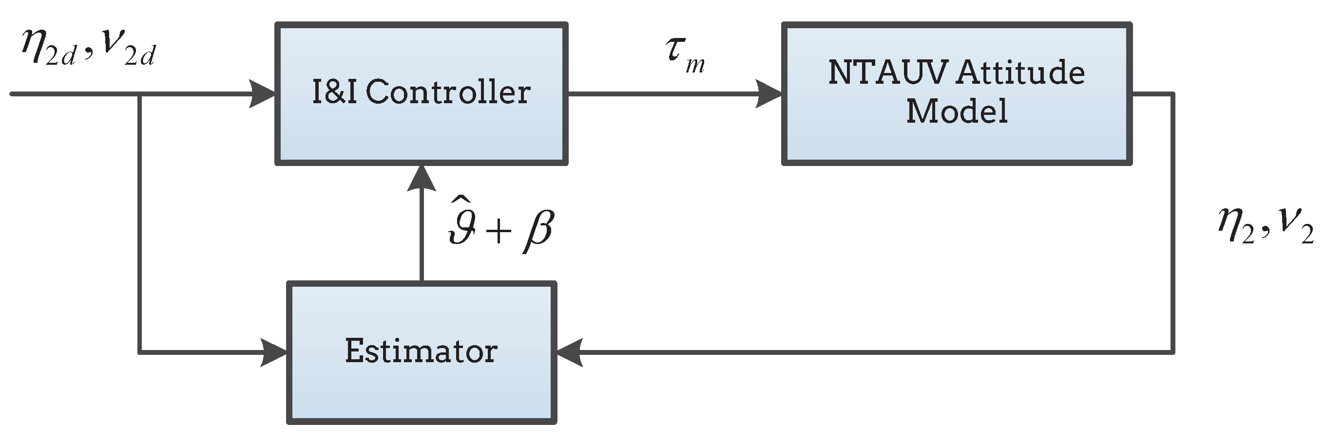
The control scheme is illustrated in Figure 2.

3.3. Stability Analysis

The derivative of (44) is

$$\begin{array}{cc}\hfill {\dot{z}}_i& ={\dot{\widehat{\vartheta }}}_i-{\dot{\vartheta }}_i+{\dot{\beta }}_i\left({\nu }_{2i}\right)\hfill \\ & =-\frac{\partial {\beta }_i}{\partial \left({\nu }_{2i}\right)}[{\dot{\nu }}_{2i}+z_i{\rho }_i\left({\nu }_{2i}\right)]+\frac{\partial {\beta }_i}{\partial \left({\nu }_{2i}\right)}\left({\dot{\nu }}_{2i}\right)\hfill \\ & =-{\gamma }_i{\rho }_i\left({\nu }_{2i}\right){\rho }_i\left({\nu }_{2i}\right)z_i\hfill \end{array}$$

(53)

where ${\vartheta }_i$ is assumed to be a constant.

The Lyapunov function is $W\left(z\right)={\Sigma }_{i=1}^3\frac{1}{{\gamma }_i}{\left|z_i\right|}^2$, then

$$\begin{array}{cc}\hfill \dot{W}\left(z\right)& ={\Sigma }_{i=1}^3\frac{2}{{\gamma }_i}{z}_i{\dot{z}}_i\hfill \\ & ={\Sigma }_{i=1}^3\frac{2}{{\gamma }_i}{z}_i(-{\gamma }_i{\rho }_i\left({\nu }_{2i}\right){\rho }_i\left({\nu }_{2i}\right)z_i)\hfill \\ & =-2{\Sigma }_{i=1}^3{z}_i{\rho }_i\left({\nu }_{2i}\right){\rho }_i\left({\nu }_{2i}\right)z_i\hfill \\ & =-2{\Delta }^{\top }\Delta \hfill \\ & =-{2|\Delta |}^2\le 0\hfill \end{array}$$

(54)

which means that $\widehat{\vartheta }\to \vartheta$ as $t\to \infty$.

We want the whole system to be stable, which means ${({\tilde{\eta }}_2,{\tilde{\nu }}_2,z)}^{\top }$ has the equilibrium point ${(0,0,0)}^{\top }$ that is stable.

Consider the Lyapunov function $V=H({\tilde{\eta }}_2,{\tilde{\nu }}_2)+W\left(z\right)$. The derivative of V is

$$\begin{array}{cc}\hfill \dot{V}& =\frac{\partial H}{\partial {\tilde{\eta }}_2}{\dot{\tilde{\eta }}}_2+\frac{\partial H}{\partial ({I\tilde{\nu }}_2)}(I{\dot{\tilde{\nu }}}_2)+\dot{W}(z)\hfill \\ & =\frac{\partial H}{\partial {\tilde{\eta }}_2}{J}_2({\eta }_2)I^{-1}\frac{\partial H^{\top }}{\partial {\tilde{\nu }}_2}+\frac{\partial H}{\partial ({I\tilde{\nu }}_2)}(-I^{-1}{J}_2^{\top }({\eta }_2)\frac{\partial H^{\top }}{\partial {\tilde{\eta }}_2}+(S({\nu }_2)-K_2)\frac{\partial H^{\top }}{\partial {\tilde{\nu }}_2}-\Delta )-2{\Delta }^{\top }\Delta \hfill \\ & =\frac{\partial H}{\partial ({I\tilde{\nu }}_2)}(-K_2\frac{\partial H^{\top }}{\partial {\tilde{\nu }}_2}-\Delta )-2{\Delta }^{\top }\Delta \hfill \\ & =-\frac{\partial H}{\partial ({I\tilde{\nu }}_2)}{K}_2\frac{\partial H^{\top }}{\partial {\tilde{\nu }}_2}-\frac{\partial H}{\partial ({I\tilde{\nu }}_2)}\Delta -2{\Delta }^{\top }\Delta \hfill \\ & =-\frac{\partial H}{\partial ({I\tilde{\nu }}_2)}(K_2-\frac{1}{2\sqrt{2}}{I}_{3\times 3})\frac{\partial H^{\top }}{\partial {\tilde{\nu }}_2}-\frac{\partial H}{\partial ({I\tilde{\nu }}_2)}(\frac{1}{2\sqrt{2}}{I}_{3\times 3})\frac{\partial H^{\top }}{\partial {\tilde{\nu }}_2}-\frac{\partial H}{\partial ({I\tilde{\nu }}_2)}\Delta -2{\Delta }^{\top }\Delta \hfill \end{array}$$

select $K_2$ such that $K_2-\frac{1}{2\sqrt{2}}{I}_{3\times 3}>0$; then, $\dot{V}\le 0$.

4. Experiment Results

4.1. Testbed

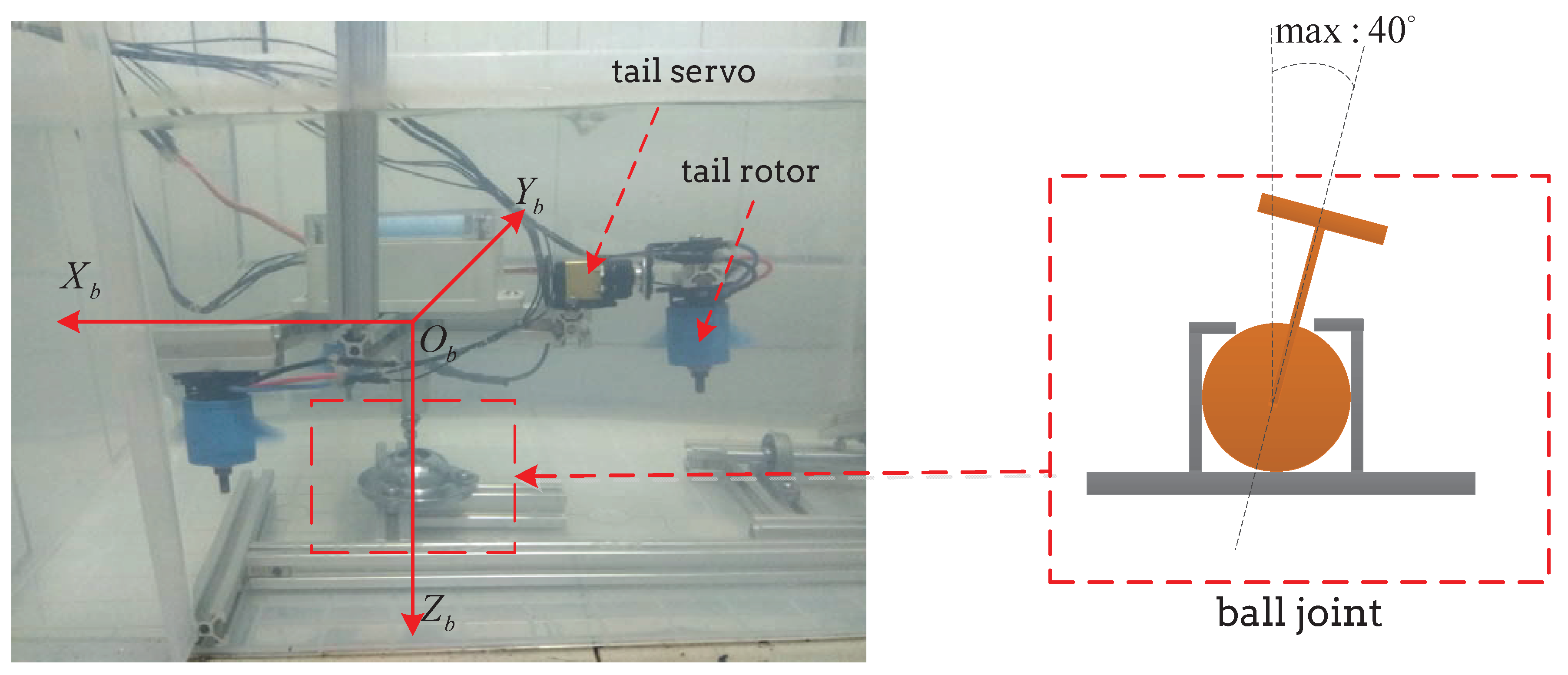
A 3 DOF testbed is designed for verifying the performance of the presented controller. The testbed includes three parts: the unmovable base, 3-DOF ball joint, and NTAUV. The ball joint enables a maximum $\pm {40}^{\circ }$ roll and pitch angle and ${360}^{\circ }$ yaw angle. The 3 DOF ball joint of the testbed is illustrated in Figure 3.

The mechanical parameters of the NTAUV are listed in

Table 1. Mechanical parameters of NTAUV.

Parameters	Value	Unit (SI)
$l_1$	0.13	m
$l_2$	0.075	m
$l_3$	0.15	m
m	1	kg
B	3	N
$I_{xx}$	0.0061	kg/m${}^2$
$I_{yy}$	0.006	kg/m${}^2$
$I_{zz}$	0.0118	kg/m${}^2$

.

We designed our own control system. A desktop PC running ground station software was used as the host computer. This computer sends commands and receives attitude data via a serial port. An STM32 Nucleo F401RE board, with 512 KB memory and 84 MHz CPU frequency is used as the controller board. The computation power guarantees the capability to apply an advanced control algorithm, dealing with complex matrix calculation running at 100 Hz.

The attitude sensor module reads raw three-axis accelerometers, gyroscopes, and magnetometers data from MPU9250, runs a Kalman filter algorithm, and sends the attitude and angular speed to the controller board. The rotor is a brushless DC motor; a propeller is mounted on the top of the motor, and it can provide maximum thrust of 15 N. The servo provides a maximum torque of 0.15 N· m, and the maximum speed of rotation is 6.9 rad/s .

4.2. Experiment Results and Discussion

Attitude control is essential for under actuated rigid body vehicles, such as airplanes, surface vessels, helicopters, and multi-rotor aerial vehicles. Attitude control is often designed as the inner loop of path or trajectory control, named as hierarchical control. ${\eta }_{2d}$ is the output of the higher layer controller. As a fundamental function of attitude control, ${\eta }_{2d}={[0,0,0]}^{\top }$ is an essential state that needs to be stabilized under the influence of disturbance, such as hydrodynamic moments generated by constant fluent or turbulence, and collision.

4.2.1. I&I Control Experiment

The parameters of the I&I controller are selected as follows: $K_1=diag\{0.02,0.1,0.03\}$, $K_2=diag\{5,5,5\}$, $\gamma ={[0.4,0.4,0.4]}^{\top }$.

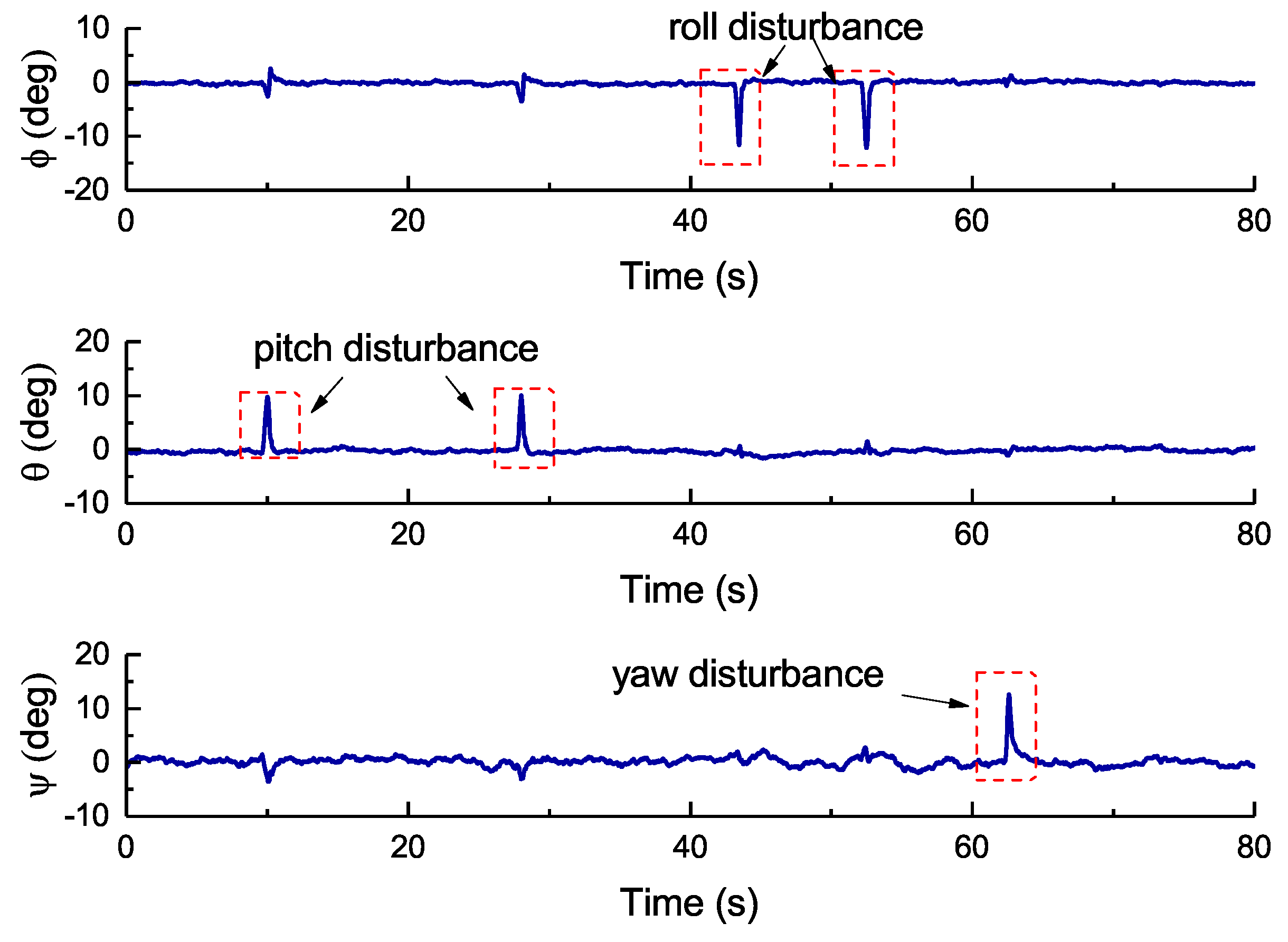
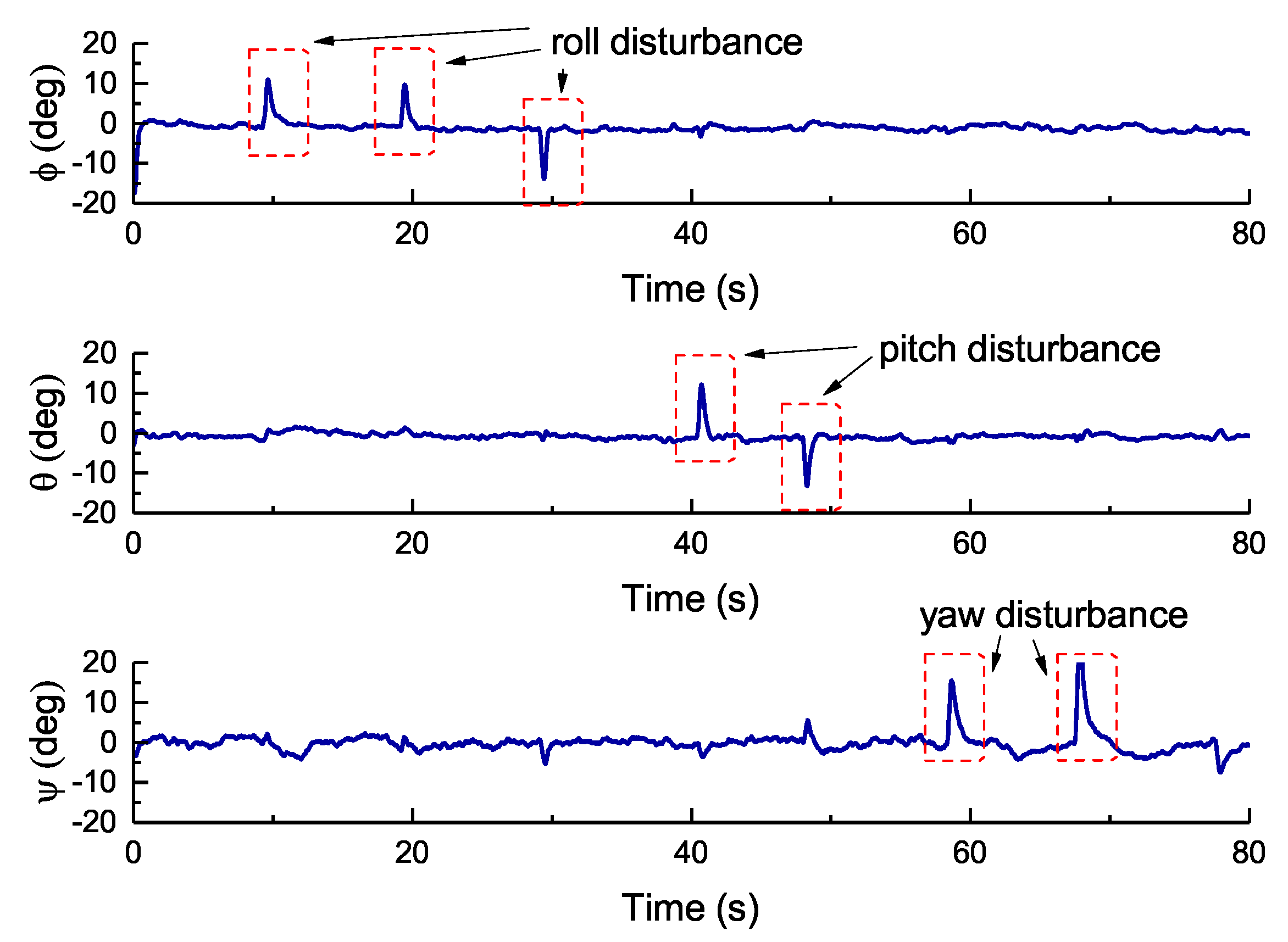
To validate the anti-disturbance performance of I&I controller, disturbances are applied to each axis. Each axis is disturbed by a collision. The I&I controller regulates the state to ${\eta }_2={[0,0,0]}^{\top }$ . The roll, pitch, and yaw control results of I&I control are shown in Figure 4.

The experiment results show that: (1) the attitude error generated by the collision is near ${10}^{\circ }$; (2) the attitude converges to ${\eta }_{2d}$ in less than 0.8 s; (3) the roll and pith control have shorter adjust time than the yaw control, which is because the yaw axis has a higher moment of inertia and a lower control moment, resulting from the mechanical design of the rotor arrangement; and (4) when no disturbance is applied, the control accuracy of roll and pitch is better than yaw; this is mainly for the unmodeled dynamics of the tail servo.

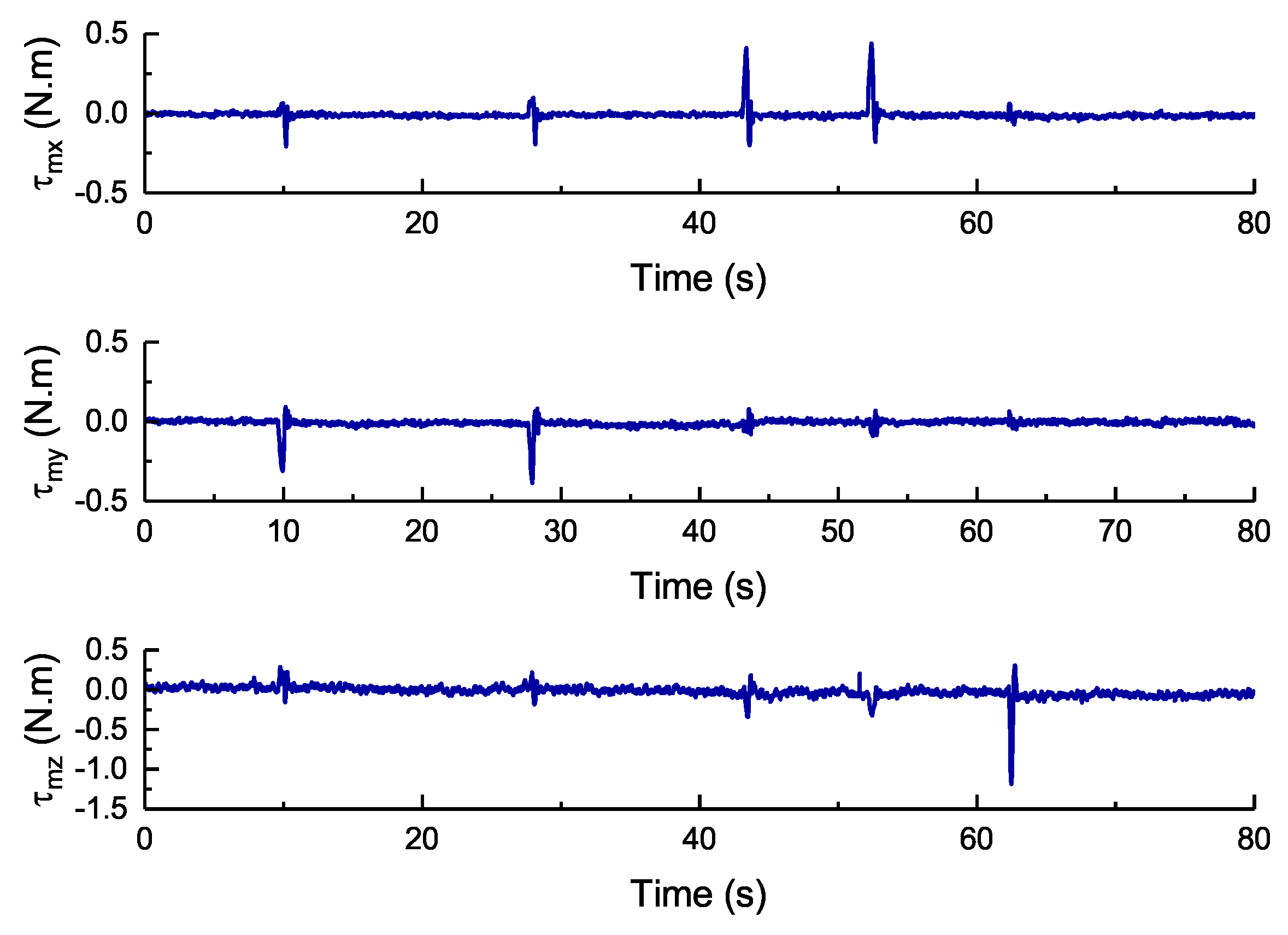
The control torque is shown in Figure 5. The roll and pitch control toques are generated by the change in the speed of the rotors, which is quick, whereas the yaw control torque is generated by the servo sway, which is slow and has a slight chattering.

4.2.2. PI Control Experiment

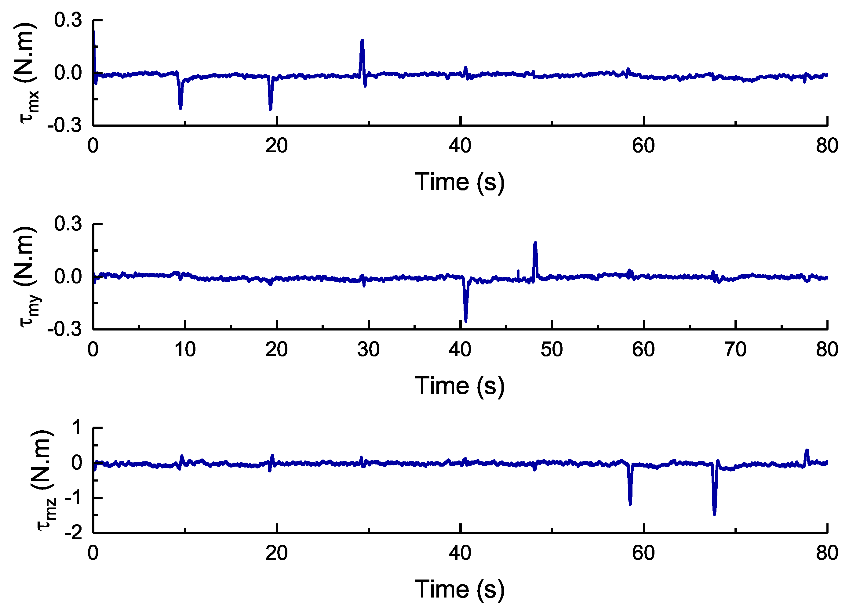
We compare experiment results generated by the I&I controller with the ones generated by the typical cascaded proportional integral (PI) controller. The parameters of PI controller are selected carefully to get good performance. The parameters of PI approach are as follows: angular velocity loop controller $k_p^v=0.2,k_i^v=1$, angular position loop controller $k_p^p=0.08,k_i^p=0.001$. The experiment results of PI control are shown in Figure 6 and Figure 7. It shows that it takes more than 1.3 s to converge to desired attitude, and the yaw control takes even more than 3 s.

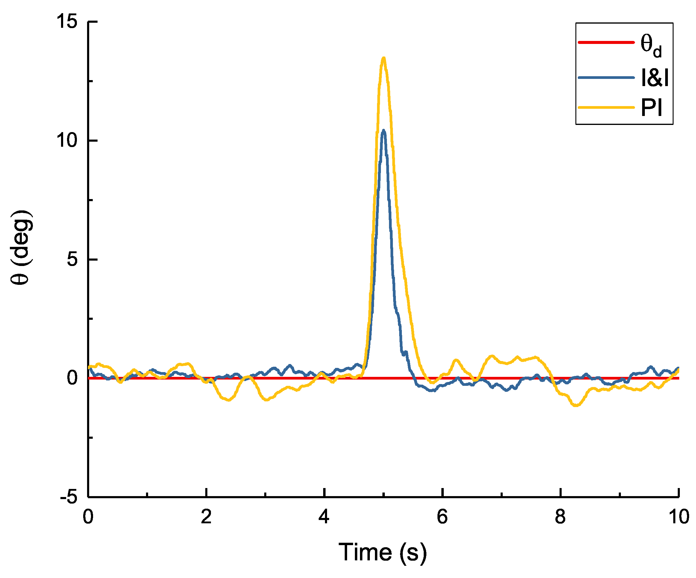
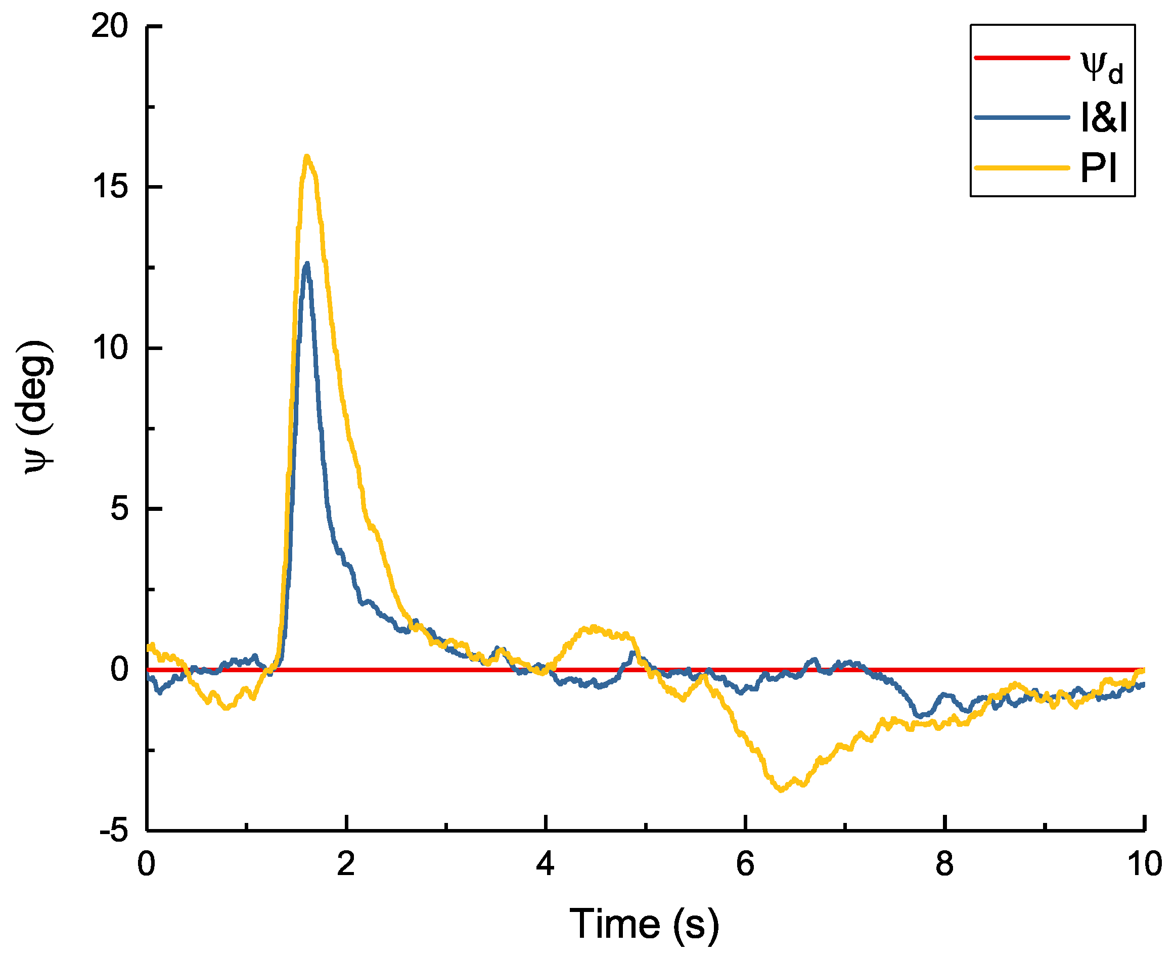
4.2.3. Comparison Between I&I and PI Control

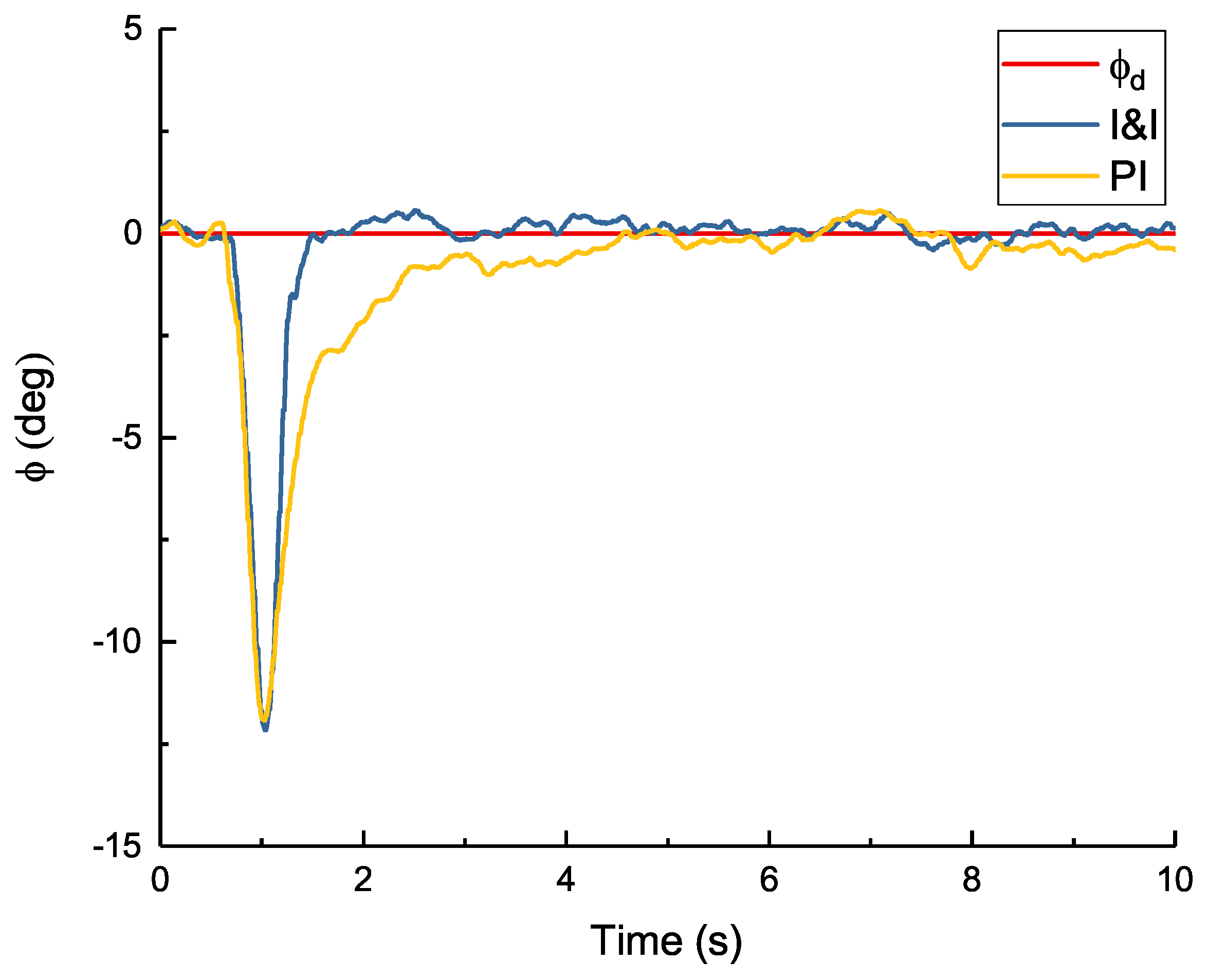
The comparisons of the roll, pitch and yaw control performance between I&I and PI control are shown separately in Figure 8, Figure 9 and Figure 10. The I&I control performs higher accuracy than PI control under disturbance.

The hydrodynamic force and moment are complex as the underwater vehicle works at a low Reynolds number (Re) condition, especially when hovering and for low-speed horizontal moving. The actual hydrodynamic force is very complex, because there is no stable flow field around. The disturbance rejection performance of I&I control is validated.

5. Conclusions

In this paper, a negative-buoyancy tri-tilt-rotor autonomous underwater vehicle was presented and an attitude controller was designed for attitude stabilization. The full mathematical model of the NTAUV was established, and it was decoupled to attitude and altitude subsystems. Then, the attitude subsystem was investigated, and an adaptive attitude controller was designed based on the I&I theory. A parameter estimator was applied to estimate the unknown parameters. The global stability of the controller was proved. Finally, the performance of the proposed controller was validated through a real-time attitude stabilization experiment. The experimental results indicated a satisfactory performance compared with a well designed PID controller.

References

- Fossen, T. Guidance and Control of Ocean Vehicles; John Willey & Sons: Hoboken, NJ, USA, 1994. [Google Scholar]
- Li, X.; Zhao, M.; Ge, T. A Nonlinear Observer for Remotely Operated Vehicles with Cable Effect in Ocean Currents. Appl. Sci. 2018, 8, 867. [Google Scholar] [CrossRef]
- Wu, N.; Wu, C.; Ge, T.; Yang, D.; Yang, R. Pitch Channel Control of a REMUS AUV with Input Saturation and Coupling Disturbances. Appl. Sci. 2018, 8, 253. [Google Scholar] [CrossRef]
- Salgado-Jimenez, T.; Gonzalez-Lopez, J.L.; Pedraza-Ortega, J.C.; García-Valdovinos, L.G.; Martínez-Soto, L.F.; Resendiz-Gonzalez, P.A. Design of ROVs for the Mexican power and oil industries. In Proceedings of the 2010 1st International Conference on Applied Robotics for the Power Industry, Montreal, QC, Canada, 5–7 October 2010; pp. 1–8. [Google Scholar]
- Soylu, S.; Proctor, A.A.; Podhorodeski, R.P.; Bradley, C.; Buckham, B.J. Precise trajectory control for an inspection class ROV. Ocean Eng. 2016, 111, 508–523. [Google Scholar] [CrossRef]
- Wynn, R.B.; Huvenne, V.A.I.; Le Bas, T.P.; Murton, B.J.; Connelly, D.P.; Bett, B.J.; Ruhl, H.A.; Morris, K.J.; Peakall, J.; Parsons, D.R.; et al. Autonomous Underwater Vehicles (AUVs): Their past, present and future contributions to the advancement of marine geoscience. Mar. Geol. 2014, 352, 451–468. [Google Scholar] [CrossRef] [Green Version]
- Palomeras, N.; Vallicrosa, G.; Mallios, A.; Bosch, J.; Vidal, E.; Hurtos, N.; Carreras, M.; Ridao, P. AUV homing and docking for remote operations. Ocean Eng. 2018, 154, 106–120. [Google Scholar] [CrossRef]
- Liu, K.; Huang, Y.; Zhao, Y.; Cui, S.; Wang, X.; Wang, G. Research on error correction methods for the integrated navigation system of deep-sea human occupied vehicles. In Proceedings of the OCEANS 2015—MTS/IEEE Washington, Washington, DC, USA, 19–22 October 2015; pp. 1–5. [Google Scholar]
- Hosseini, M.; Seyedtabaii, S. Robust ROV path following considering disturbance and measurement error using data fusion. Appl. Ocean Res. 2016, 54, 67–72. [Google Scholar] [CrossRef]
- Cui, R.; Zhang, X.; Cui, D. Adaptive sliding-mode attitude control for autonomous underwater vehicles with input nonlinearities. Ocean Eng. 2016, 123, 45–54. [Google Scholar] [CrossRef]
- Cui, R.; Li, Y.; Yan, W. Mutual Information-Based Multi-AUV Path Planning for Scalar Field Sampling Using Multidimensional RRT. IEEE Trans. Syst. Man Cybern. Syst. 2016, 46, 993–1004. [Google Scholar] [CrossRef]
- Cui, R.; Yang, C.; Li, Y.; Sharma, S. Adaptive Neural Network Control of AUVs With Control Input Nonlinearities Using Reinforcement Learning. IEEE Trans. Syst. Man Cybern. Syst. 2017, 47, 1019–1029. [Google Scholar] [CrossRef]
- Nouri, N.M.; Valadi, M. Robust input design for nonlinear dynamic modeling of AUV. ISA Trans. 2017, 70, 288–297. [Google Scholar] [CrossRef] [PubMed]
- Paull, L.; Saeedi, S.; Seto, M.; Li, H. AUV Navigation and Localization: A Review. IEEE J. Ocean. Eng. 2014, 39, 131–149. [Google Scholar] [CrossRef]
- Hussain, N.A.A.; Arshad, M.R.; Mohd-Mokhtar, R. Underwater glider modelling and analysis for net buoyancy, depth and pitch angle control. Ocean Eng. 2011, 38, 1782–1791. [Google Scholar] [CrossRef]
- Brown, C.L. Deep sea mining and robotics: Assessing legal, societal and ethical implications. In Proceedings of the 2017 IEEE Workshop on Advanced Robotics and its Social Impacts (ARSO), Austin, TX, USA, 8–10 March 2017; pp. 1–2. [Google Scholar]
- Javaid, M.Y.; Ovinis, M.; Hashim, F.B.M.; Maimun, A.; Ahmed, Y.M.; Ullah, B. Effect of wing form on the hydrodynamic characteristics and dynamic stability of an underwater glider. Int. J. Naval Archit. Ocean Eng. 2017, 9, 382–389. [Google Scholar] [CrossRef]
- Li, Y.; Pan, D.; Zhao, Q.; Ma, Z.; Wang, X. Hydrodynamic performance of an autonomous underwater glider with a pair of bioinspired hydro wings—A numerical investigation. Ocean Eng. 2018, 163, 51–57. [Google Scholar] [CrossRef]
- Tchilian, R.D.S.; Rafikova, E.; Gafurov, S.A.; Rafikov, M. Optimal Control of an Underwater Glider Vehicle. Procedia Eng. 2017, 176, 732–740. [Google Scholar] [CrossRef]
- Bessa, W.M.; Dutra, M.S.; Kreuzer, E. An adaptive fuzzy sliding mode controller for remotely operated underwater vehicles. Robot. Auton. Syst. 2010, 58, 16–26. [Google Scholar] [CrossRef]
- Campos, E.; Monroy, J.; Abundis, H.; Chemori, A.; Creuze, V.; Torres, J. A nonlinear controller based on saturation functions with variable parameters to stabilize an AUV. Int. J. Naval Archit. Ocean Eng. 2018. [Google Scholar] [CrossRef]
- Yan, H.; Ge, T.; Li, J.W.; Wang, Q. Prediction of mode and static stability of negative buoyancy vehicle. In Proceedings of the 2011 Chinese Control and Decision Conference (CCDC), Mianyang, China, 23–25 May 2011; pp. 1903–1909. [Google Scholar]
- Ji, S.W.; Bui, V.P.; Balachandran, B.; Kim, Y.B. Robust control allocation design for marine vessel. Ocean Eng. 2013, 63, 105–111. [Google Scholar] [CrossRef]
- Xiang, X.; Lapierre, L.; Jouvencel, B. Smooth transition of AUV motion control: From fully-actuated to under-actuated configuration. Robot. Auton. Syst. 2015, 67, 14–22. [Google Scholar] [CrossRef] [Green Version]
- Xiang, X.; Yu, C.; Zhang, Q. Robust fuzzy 3D path following for autonomous underwater vehicle subject to uncertainties. Comput. Oper. Res. 2017, 84, 165–177. [Google Scholar] [CrossRef]
- Salazar-Cruz, S.; Kendoul, F.; Lozano, R.; Fantoni, I. Real-time stabilization of a small three-rotor aircraft. IEEE Trans. Aerosp. Electron. Syst. 2008, 44, 783–794. [Google Scholar] [CrossRef]
- Papachristos, C.; Tzes, A. Modeling and control simulation of an unmanned Tilt Tri-Rotor Aerial vehicle. In Proceedings of the 2012 IEEE International Conference on Industrial Technology, Athens, Greece, 19–21 March 2012; pp. 840–845. [Google Scholar]
- Ta, D.A.; Fantoni, I.; Lozano, R. Modeling and control of a tilt tri-rotor airplane. In Proceedings of the 2012 American Control Conference (ACC), Montreal, QC, Canada, 27–29 June 2012; pp. 131–136. [Google Scholar]
- Astolfi, A.; Ortega, R. Immersion and invariance (I2): A new tool in nonlinear control design. In Proceedings of the 2001 European Control Conference (ECC), Porto, Portugal, 4–7 September 2001; pp. 2854–2859. [Google Scholar]
- Astolfi, A.; Ortega, R. Immersion and invariance: A new tool for stabilization and adaptive control of nonlinear systems. IEEE Trans. Autom. Control 2003, 48, 590–606. [Google Scholar] [CrossRef]
- Astolfi, A.; Karagiannis, D.; Ortega, R. Nonlinear and Adaptive Control with Applications; Springer: Berlin/Heidelberg, Germany, 2008. [Google Scholar]
Figure 1.
Configuration of NTAUV with Earth-fixed and body-fixed frame.
Figure 2.
I&I control scheme.
Figure 3.
Testbed.
Figure 4.
Attitude of NTAUV under I&I control with disturbance on each axis.
Figure 5.
I&I control torque.
Figure 6.
Attitude of NTAUV under PI control with disturbance on each axis.
Figure 7.
PI control torque.
Figure 8.
Roll Control Comparison between I&I and PI Control.
Figure 9.
Pitch Control Comparison between I&I and PI Control.
Figure 10.
Yaw Control Comparison between I&I and PI Control.