An Integration Strategy for Acoustic Metamaterials to Achieve Absorption by Design


Department of Physics, Hong Kong University of Science and Technology, Clear Water Bay, Kowloon, Hong Kong, China
*
Author to whom correspondence should be addressed.
Appl. Sci. 2018, 8(8), 1247; https://doi.org/10.3390/app8081247
Submission received: 12 June 2018
/
Revised: 2 July 2018
/
Accepted: 23 July 2018
/
Published: 27 July 2018
(This article belongs to the Special Issue Acoustic Metamaterials)
Abstract
:As much of metamaterials’ properties originate from resonances, the novel characteristics displayed by acoustic metamaterials are a narrow bandwidth and high dispersive in nature. However, for practical applications, broadband is often a necessity. Furthermore, it would even be better if acoustic metamaterials can display tunable bandwidth characteristics, e.g., with an absorption spectrum that is tailored to fit the noise spectrum. In this article we present a designed integration strategy for acoustic metamaterials that not only overcomes the narrow-band Achilles’ heel for acoustic absorption but also achieves such effect with the minimum sample thickness as dictated by the law of nature. The three elements of the design strategy comprise: (a) the causality constraint, (b) the determination of resonant mode density in accordance with the input target impedance, and (c) the accounting of absorption by evanescent waves. Here, the causality constraint relates the absorption spectrum to a minimum sample thickness, derived from the causal nature of the acoustic response. We have successfully implemented the design strategy by realizing three structures of which one acoustic metamaterial structure, comprising 16 Fabry-Perot resonators, is shown to exhibit near-perfect flat absorption spectrum starting at 400 Hz. The sample has a thickness of 10.86 cm, whereas the minimum thickness as dictated by the causality constraint is 10.55 cm in this particular case. A second structure demonstrates the flexible tunability of the design strategy by opening a reflection notch in the absorption spectrum, extending from 600 to 1000 Hz, with a sample thickness that is only 3 mm above the causality minimum. We compare the designed absorption structure with conventional absorption materials/structures, such as the acoustic sponge and micro-perforated plate, with equal thicknesses as the metamaterial structure. In both cases the designed metamaterial structure displays superior absorption performance in the target frequency range.
1. Introduction
Even in the 21st century, acoustic noise can still be a pernicious problem. An obvious question facing the scientific and engineering community is: How can we do better to remediate this problem? While doing by trial and error and learning by experience clearly constitute a path forward, occasionally natural laws can offer us the ultimate limit on how well one can achieve. It is the purpose of this article to show that acoustic absorption is one such case, and knowing the limit represents a tremendous advantage since one can work backwards in designing strategies to achieve such limit. The relevant limit in the case of acoustic absorption is that imposed by the causality principle, which, combined with the resonant mode density determination based on the target absorption spectrum for a structure backed by a reflecting substrate, is shown to yield a self-consistent strategy for achieving absorption by design. By considering the absorption through evanescent waves, we also address the practical issue of using a finite number of resonances to best achieve the target absorption spectrum.
For absorption at least, our design approach presented in this article has overcome the Achilles’ heel of narrow frequency bandwidth and dispersive character [1,2] for acoustic metamaterials.
Acoustic response of materials and/or structures must obey the causality principle, which states that the response at any moment of time can only depend on what occurred prior to that moment. In other words, the future cannot affect what happens now. Translated into mathematical language, this simple and intuitive statement can have deep consequences. In 1926–1927, Hans Kramers and Ralph Kronig independently derived the well-known Kramers-Kronig relationship between the real and imaginary parts of the dielectric function for electromagnetic waves, based on the causality principle [3]. Another, much less-known consequence of the causality principle is that for any electromagnetic absorption spectrum, there is a minimum sample thickness [4,5]. Adapted to acoustics, we have derived the following relationship for a flat structure sitting on a reflecting substrate [6]:
Here, denotes the sound wavelength in air, with being the speed of air-borne sound, the angular frequency, the absorption spectrum, the effective bulk modulus of the sound absorbing structure in the static limit, and the bulk modulus of air. For the sake of making the present article self-contained, we give a detailed derivation of Equation (1) in Appendix A that first appeared in the Supplementary Information section of ref. [6]. Equation (1) tells us that the acoustic absorption spectrum cannot be independent from the sample thickness. A somewhat interesting aspect of Equation (1) is that only the bulk modulus appears in the causality constraint (in the electromagnetic case only the magnetic permeability appears in the causality constraint), whereas it is well known in acoustics that there are two material parameters: bulk modulus and mass density. This is attributed to the fact that in the derivation, it is necessary to take the zero-frequency limit. Hence, no inertial effect can be present. Some immediate implications of Equation (1) are that there cannot be 100% absorption over a finite frequency range by a finite-thickness structure, and that closer the absorption gets to 100%, the thicker the sample must be. Also, for the same frequency bandwidth, a lower central frequency implies a thicker minimum sample thickness, and vice versa.
It should be mentioned that there have been numerous studies to broaden the frequency range of absorption for acoustic metamaterials, some of which were quite successful [7,8,9,10]. The present approach differs by delineating the ultimate limit as dictated by natural law, and using such constraint as part of the design strategy to achieve tunable absorption by design.
2. Turning the Causality Constraint into a Design Tool
By setting in Equation (1), we can interpret the resulting equation as a design tool. That is, one can use the equation to find the solution to the following questions. For a given sample thickness d and a fixed frequency (wavelength) range, what is the best absorption achievable? From the causality constraint, it is clear that for a given sample thickness, there is only a limited amount of absorption resources. Therefore, in this context the real question is: How to allocate these limited resources, i.e., how to define “best”? If the purpose is noise remediation, then perhaps the best target absorption spectrum is that which matches the noise spectrum. Alternatively, for a fixed d and a desired absorption level, what is the broadest possible frequency range possible? But perhaps the most-often encountered scenario would be: For a target absorption spectrum , what would be the minimum sample thickness achievable? Below we show examples for what can be achieved from this perspective, but first it is necessary to consider the requirement of impedance matching for a sample, which is the complementary consideration to the causality constraint in our strategy to design a structure with a tunable absorption spectrum.
We define any sound absorption sample to be “optimal” if it attains .
3. Impedance, Absorption and Green Function
At normal incidence, reflection coefficient R from a flat sample is given by
where denotes the sample impedance, is the mass density, and v is the sound speed. Here, is the impedance of air. If the sample sits on a reflecting hard surface, then there is no transmission, and absorption A can be directly calculated as . In other words, there is a one-to-one correspondence between absorption and the impedance ratio . In what follows, we consider how this impedance ratio can be tuned via acoustic resonances, i.e., through the use of metamaterials.
Impedance and Green Function
When the lateral sample dimension is much smaller than the wavelength so that the diffraction effect can be neglected, impedance may be alternatively defined as
where p denotes pressure modulation, and is the displacement velocity. The Green function is defined as
Hence, for harmonic waves we have a simple relationship between the impedance and the Green function:
i.e., the two are essentially the inverse of each other, with the real and imaginary parts switched. The advantage of expressing the impedance in this manner is that the Green function can be explicitly written down through the eigenfunction expansion approach. For the acoustic metamaterials, the eigenfunctions are the resonance modes, which must have the Lorentzian form. To illustrate how the resonance can tune the impedance, let us consider the case of a system having two discrete resonances with resonance frequencies :
where denotes the density of air, and is the oscillator strength, to be made explicit later. Here, we treat the dissipation to be negligibly small. It is clear that at the impedance is zero, and there is always a frequency where the sum of the two terms vanishes in the parenthesis, so that the magnitude of the impedance diverges. This is denoted the antiresonace point [11]. Hence, with resonances one can tune the impedance of a resonant metamaterial structure at will by varying the frequency. Since there is a one-to-one correspondence between the impedance and absorption, it follows that one might be able to obtain absorption by design, by properly integrating together multiple resonances. Below we show precisely how this proper integration can be carried out in accordance with the desired target absorption spectrum, and how the causality equality can be used to fix a crucial design parameter so as to achieve consistency with the goal of attaining absorption by design with the minimum sample thickness.
4. Integration Strategy for Achieving Absorption by Design
In order to be concrete, in the following we will consider the use of Fabry-Perot (FP) resonators to realize our integration strategy.
A simple-minded approach to putting together multiple resonances for achieving, e.g., broad-band absorption, is by integrating within a single metamaterial unit multiple resonators with equally-spaced resonance frequencies. However, we show below that there is a much better strategy than using equally-spaced resonances. To see how such a strategy can be derived, let us consider an idealized structure with a continuum of resonances so that its impedance can be written as [12]
where is the density of the resonant modes, and is the dissipative constant that controls the width of the absorption peak. It should be noted that letting does not imply the system to have zero dissipation when integrated over frequency, since a zero means that the imaginary part of the quantity in the square bracket becomes a delta function with zero width, but which has a non-zero integrated effect. It follows that from Equation (7) we have
Here, the symbol denotes taking the principal value. In Equation (8), the integrant in the imaginary part is oscillatory in nature. Hence, it can be small. If for the moment we ignore the imaginary part in the square bracket and focus only on the real part, then
Here, the mode density can be written as , where is a continuous variable that indexes the resonance modes, defined as , with n being an integer ranging from 1 to N. By recognizing that for the lowest-order FP resonances, from Equation (9) we obtain the following simple differential equation for determining the mode density from the target impedance:
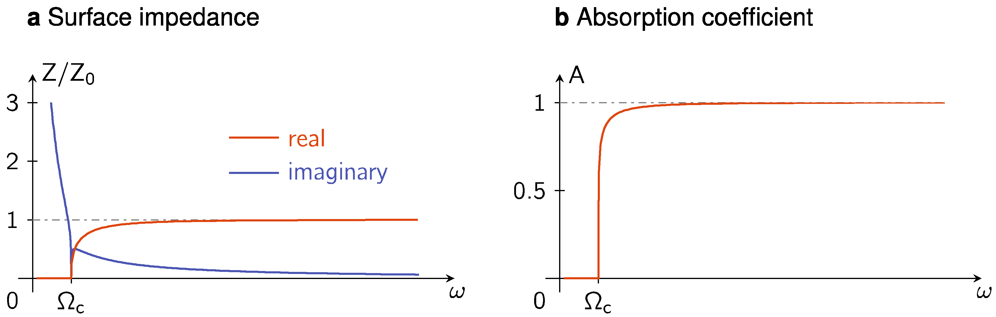
Here, is the area fraction of the FP resonators’ openings in the total surface area of the metamaterial unit. It will be seen that the determination of requires the causal relationship to achieve both minimum sample thickness as well as consistency with the target absorption spectrum. Two comments are in order. First, since we want to target a certain absorption spectrum, then can be directly obtained from Equation (2) and the fact that . Second, the mode density obtained by solving Equation (10) cannot exactly reproduce the target absorption spectrum because in the derivation of Equation (10) we have ignored the imaginary part of the impedance. In order to illustrate this point, let us choose for the target absorption spectrum a flat, perfect absorption spectrum starting at a lower cutoff frequency . In that case above and we have . Then, is a constant, and Equation (7) can be integrated to obtain:
This expression is graphically illustrated in Figure 1 below.
From Equation (11) one can easily evaluate as defined by Equation (1). If we take the effective medium expression for , then .
So far we have neglected the effects of the higher order resonances in the FP resonators, which would become more numerous as frequency increases. This is done for the clarity of presentation so that the main thesis of this work can be cleanly delineated without the complications of mathematical details, which are reproduced in Appendix B.
To complete the description of the integration strategy, we now focus on the determination of the value for through the condition of and Equation (1). For the total absorption example described above, gives the optimal form for the distribution of the resonance frequencies. If we specialize to the case of a discrete number of resonators, e.g., by using 16 FP resonators as a single, 4 × 4 acoustic metamaterial unit, then N = 16, and the length of the nth FP resonator is given by . If we can fold the longer FP resonators so as to make the metamaterial unit a compact cuboid, then the minimum thickness of the unit is determined by volume conservation, i.e.,
In Equation (12), the final expression is noted to be exact when N . By setting , one obtains an explicit expression for :
It is noted that since is calculated by using the target absorption spectrum, hence self-consistency is achieved, simultaneous with attaining the minimum sample thickness. It is clear that sets the channel length for each FP resonator. It also plays a role in the area fraction of the reflecting surface. One might ask what happens if deviates from its optimal value. For example, if one makes smaller, it is clear from Equation (12) that can be smaller. However, the price to pay is that the resulting absorption spectrum would deviate from the target absorption spectrum.
The most important consequence of neglecting the higher order FP resonances is in the determination of the value, as well as in the form for the distribution of the resonance frequencies. If we use as the target absorption spectrum the one described above, then the consideration of all the higher order FP resonances (shown in Appendix B) would lead to a value of = 0.982. Also, whereas in the above we have derived an expression , the inclusion of higher order modes makes super-linear in . Here denotes the lowest-order FP resonance, and hence it is inversely proportional to the FP channel length. Since = 0.982 implies very thin walls separating the different FP channels, in actual implementation it is necessary to deviate from this optimal value. However, there is nothing to prevent us from setting the FP channel lengths by using the correct optimal value of in conjunction with the corrected distribution, which would guarantee maximum consistency. The area fraction of the reflecting surface, however, would be larger in such case, which implies some degradation in the absorption performance from the optimal target.
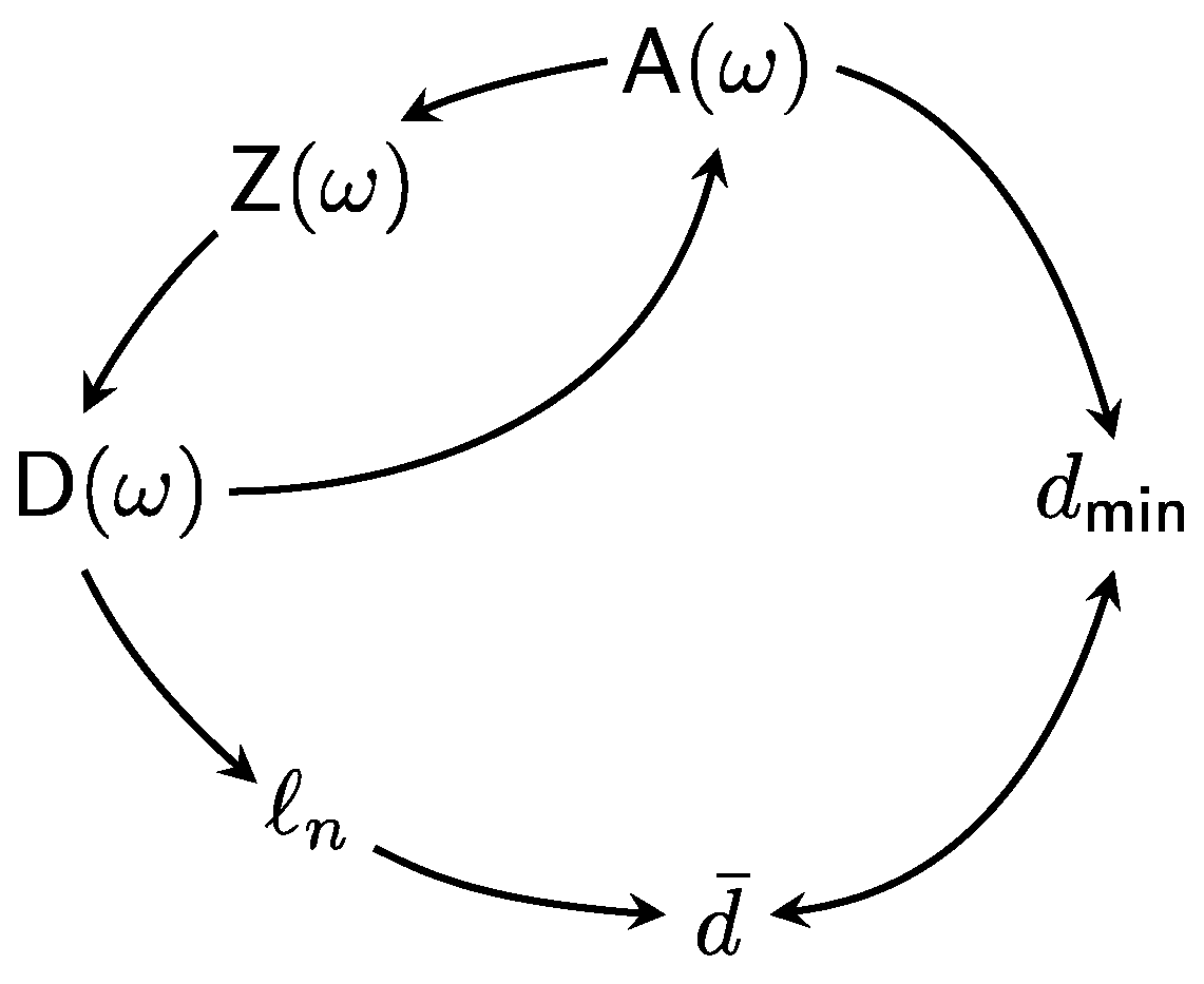
The above scheme can be schematically illustrated below by the “circle of consistency” shown in Figure 2.
It should be noted that while we have used a particular target absorption spectrum as an example (flat, total absorption for frequencies greater than ), the design strategy presented above is applicable to any desired target absorption spectrum.
5. Adverse Effect of a Finite Number of Resonators and Its Remediation
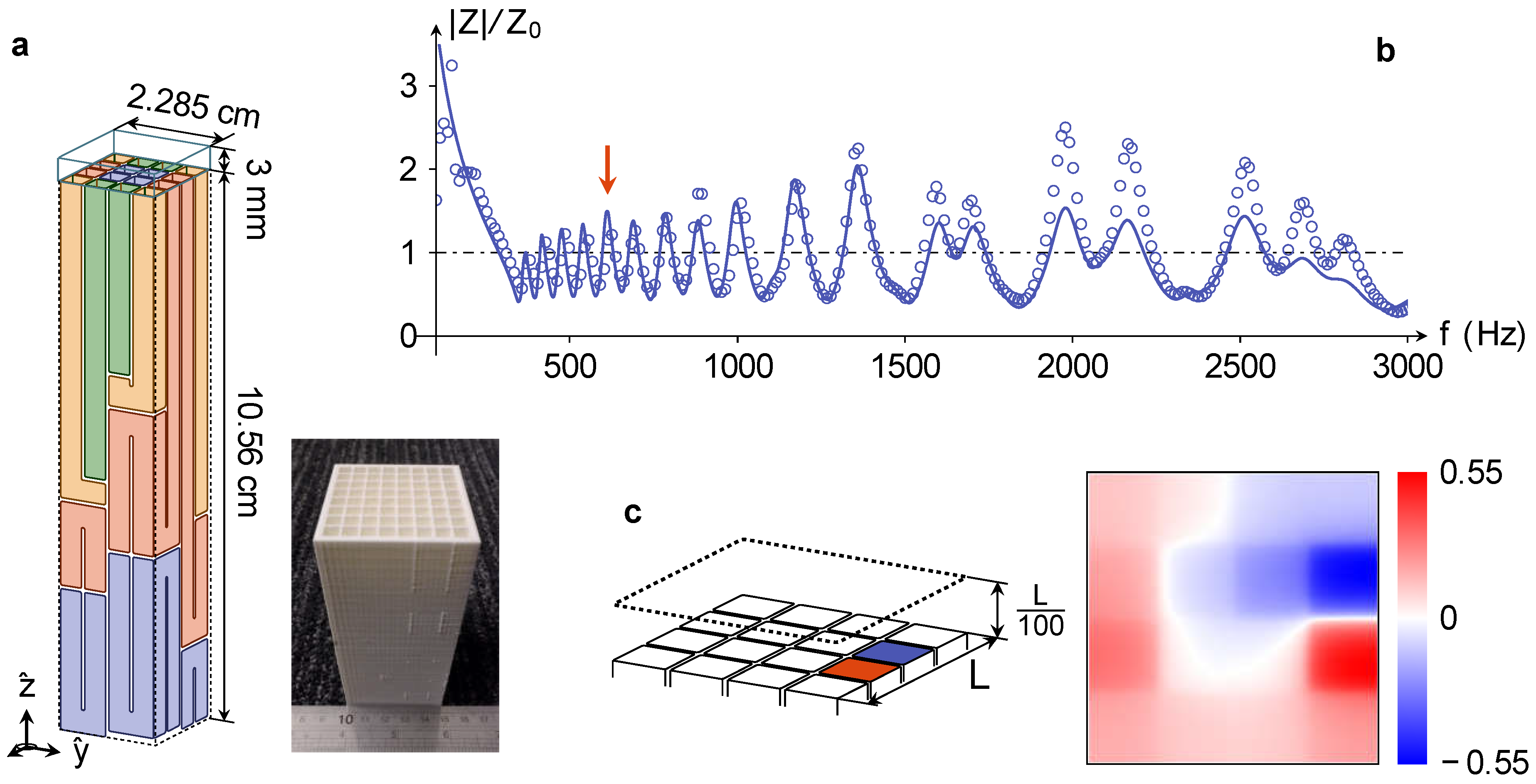
In any actual implementation of the above design strategy, it is always the case that there can only be a discrete, finite number of resonators. In Figure 3a we show an illustration and a photo image of an acoustic metamaterial unit comprising 16 FP channels, designed in accordance with the integration strategy presented in the previous section and fabricated by 3D-printed polyactide. As we cannot fabricate the sample with the wall thickness as thin as that required by the = 0.982 requirement, the final measured results are affected by the increased reflection surface due to the thicker walls. However, the effect is minimal. In Figure 3b, we plot the measured impedance as a function of frequency by blue circles. The solid line represents the analytical theory given below. Oscillations around are seen. This is the consequence of having only 16 resonators, which are not enough to insure a smooth, flat absorption spectrum. Since deviation from impedance matching implies imperfect absorption, we expect oscillations in the absorption spectrum as well.
In order to remedy the oscillations, we look into the underlying cause of a peak, indicated by the red arrow in Figure 3b. By using COMSOL to carry out full-waveform simulations, we obtained the picture shown in Figure 3c. It turns out that at the indicated peak frequency, the pressure modulation at a little distance away from the surface of the metamaterial unit is as shown in the right panel in Figure 3c. The most important feature is that there is lateral pressure modulation which averages to zero over the surface. Since the lateral size of the metamaterial unit is much less than the relevant wavelength range, such lateral pressure modulation feature implies lateral wavevector values much larger than the sound wavevector in air, . Since , at the indicated frequency the wave must decay exponentially away from the surface of the metamaterial unit, i.e., is purely imaginary. This is precisely the characteristic of the anti-resonance point. Moreover, as the right-hand side panel shows, lateral pressure modulations imply lateral oscillating pressure gradient. This intuitively tells us that there are interactions between the FP resonators. Hence, theoretically the individual Green function of the resonator should be renormalized by a self-energy term arising from the interactions, so that
where the last term on the right-hand side is the self-energy term, with denoting the bare Green function and denoting the renormalized effective Green function of the nth resonator. Here, we have used the expression for the effective mass density of a porous medium, with being the density of air, being a dimensionless parameter on the order of 1, to account for the tortuosity of the pores, and being the dissipative coefficient particular to the porous medium. The value of is fairly small for air, so we have neglected it in the expression for the bare Green function. The expression for is derived in Appendix C. The blue theoretical curve in Figure 3b is calculated by using the following formula since the 16 FP resonators are integrated in parallel; hence, the inverse of the impedance (which is just the Green function apart from the factor ) must be additive:
Very good agreements with the experiment are seen in Figure 3b and Figure 4, both shown as solid lines.
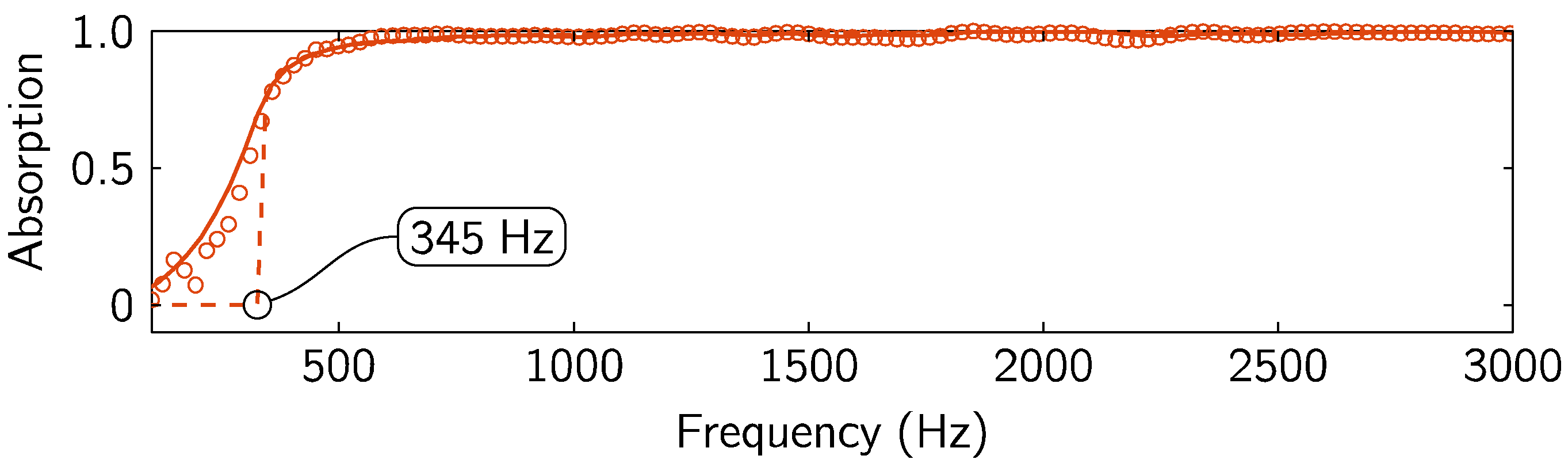
There is a reason why we use the effective mass density for a porous medium in Equation (14). Since there are lateral pressure gradient oscillations, in practical terms it can imply lateral displacement of air on the surface of the metamaterial unit at the anti-resonance point. Hence, a thin layer of acoustic sponge placed on top of the acoustic metamaterial unit can serve as a very effective absorber at the anti-resonance point. This expectation is indeed borne out, as shown by the absorption performance of the metamaterial unit in Figure 4, after a 3 mm thick layer of acoustic sponge is placed on top of the metamaterial unit. For this particular example, the sample thickness d = 10.86 cm, whereas cm. Hence, the sample is only 3 mm over the minimum thickness as dictated by the causal constraint.
For the particular sample shown in Figure 4, one may ask how far the near-perfect absorption can be extended to the higher frequencies, beyond those shown in the figure, which is 3000 Hz as limited by the impedance tube measurement. In Appendix B we show analytically that owing to the plurality of the higher-order resonances of the FP resonators and their equally-spaced frequency characteristics, the absorption actually becomes better and better with increasing frequency and approaches 1 in an exponential fashion (see Equation (A17)). Such behavior is actually substantiated by numerical simulations up to 8000 Hz.
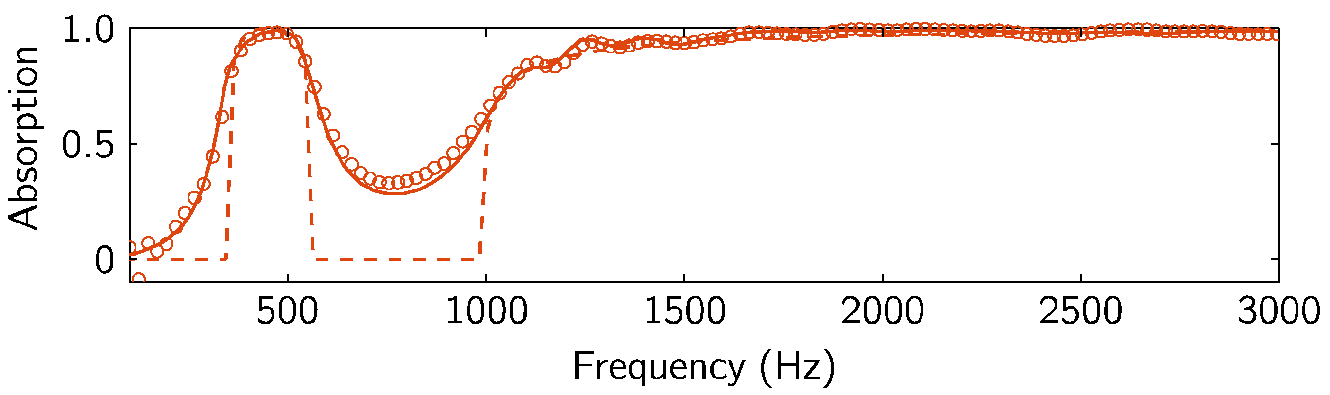
As an illustration of our integration strategy to attain the goal of absorption-by-design, in Figure 5 we show the performance of another sample with a reflection “notch” in its absorption spectrum. Again, theory and experimental results show excellent agreement. Here, the sample thickness d = 9.33 cm, whereas cm.
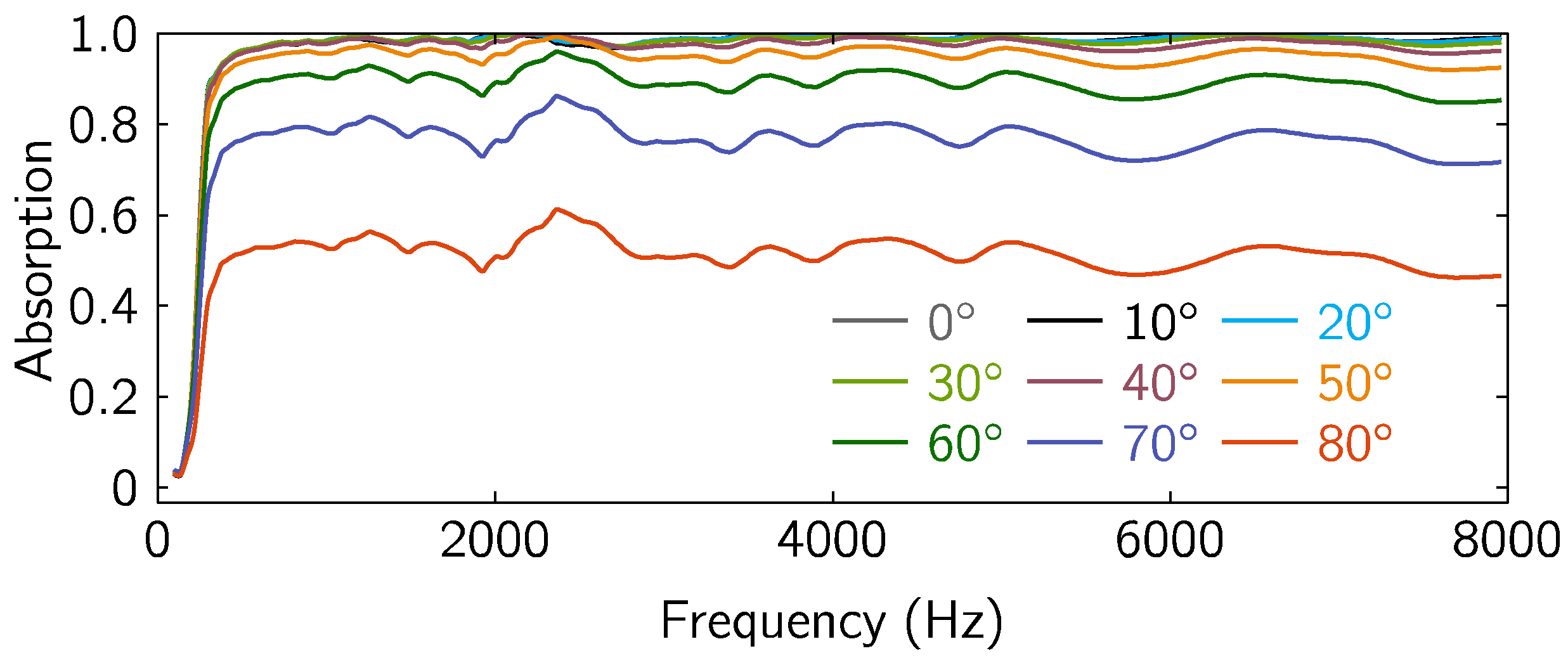
It should be mentioned that owing to the subwavelength lateral dimension of our metamaterial units, the angular dependence of absorption is nearly flat up to 60 degrees. After that the absorption smoothly drops as the angle of incidence approaches 90 degrees. Such behavior is shown by simulation results presented in Appendix D.
6. Comparison with Conventional Acoustic Absorbers
It has to be emphasized that causal optimality can be attained in conventional acoustic absorbers such as micro-perforated panel (MPP) and acoustic sponge [13]. However, they lack freedom for adjusting the absorption spectrum to a dictated target. Therefore, within the same thickness, although the causal integral Equation (1) can give the same value, the proposed absorption-by-design strategy can concentrate the absorption resources into the frequency region of interest, e.g., the peak region in the noise spectrum, thereby achieving better noise remediation.
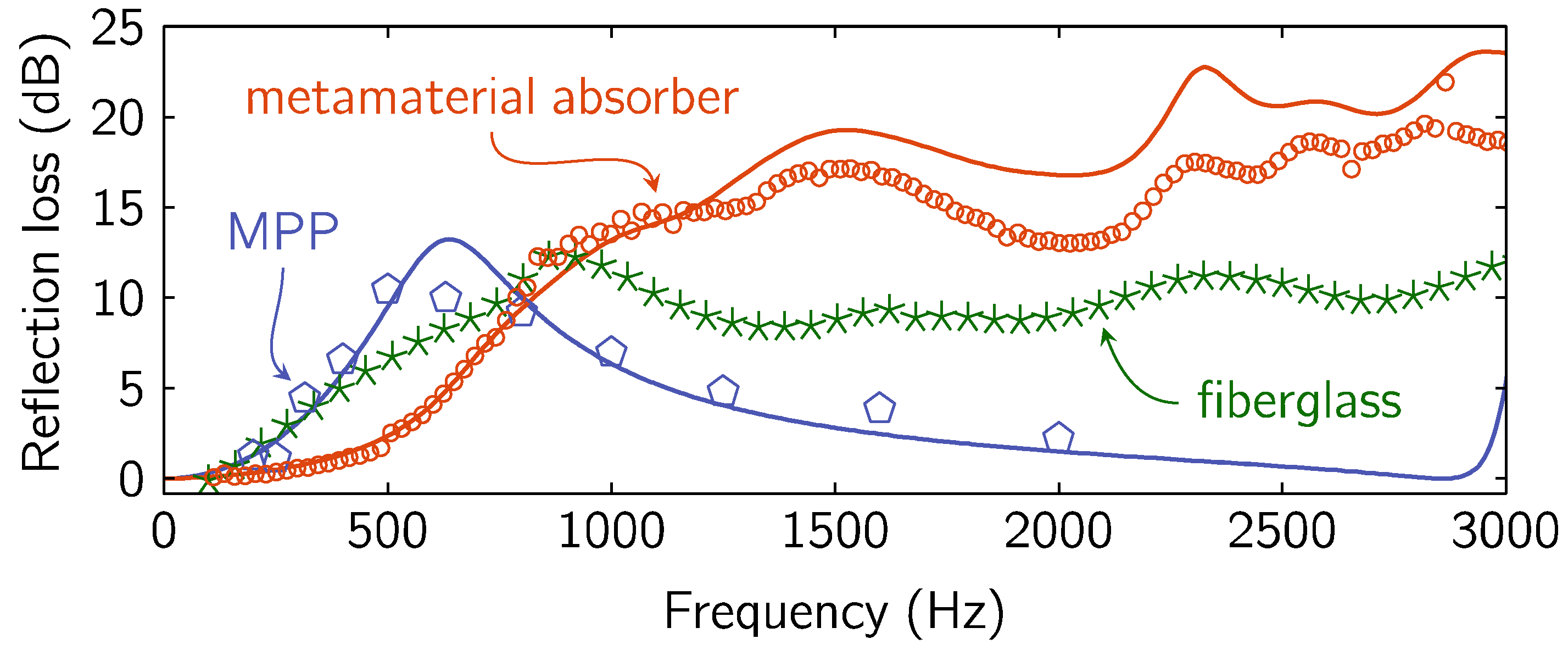
MPP is a well-known conventional resonance absorber, utilizing the acoustic resonance of the back cavity to enhance the dissipation provided by the micro-pores in the front panel. It can achieve relatively high absorption at low frequencies. In the original paper of Maa [14,15], an MPP comprising a 0.2 mm-thick aluminum plate perforated by 0.2 mm diameter circular holes with an area fraction of 2%, backed by a 6 cm cavity, can display an absorption spectrum as shown by the blue symbols (experiment) and blue line (theory) in Figure 6. The absorption peaks at 640 Hz and rapidly drop away at higher frequencies. In contrast, fiberglass is a commonly used porous material that dissipates sound by the frictions in its porous structures. Its absorption is thereby naturally broadband. A layer of 6-cm thick fiberglass (denoted by green symbols) is noted to have a flat absorption around 90% (10 dB) for frequencies higher than 800 Hz. Compared with the designed metamaterial absorber with the same thickness (5.63-cm metamaterial with 3 mm sponge in front), shown by the red circles (experiment) and line (theory), it is clear that within the target absorption frequency range of above 800 Hz, our designed metamaterial structure is 5 to 10 dB better than the fiberglass. This is achieved precisely by concentrating the absorption resources in the target frequency regime.
The above comparisons emphasize the point that under the constraint of causality, the absorption-by-design approach can provide an efficient way to utilize the limited absorption resources to achieve the optimal sound attenuation in frequencies of interest. This feature is particularly essential for solving noise problems in mechanical systems like large machines, transformers, and aircraft engines, etc., in which the noise is broadband but with featured spectra.
7. Conclusions
In this work we have presented a new approach, comprising the use of causality constraint and impedance matching to the target absorption spectrum, for the fabrication of acoustic metamaterial structures that can display for the first time the desired absorption by design tunability, without a theoretical upper frequency limit. The whole design concept can be summarized by a circle of consistency (Figure 2), and the implementation by using 3D-printed FP resonator structures has yielded measured results in excellent agreement with the theory prediction. A theoretical formalism for treating the evanescent waves is also presented, which not only can accurately predict the shifts in the resonance frequencies of the FP resonators when they are placed in close proximity to each other, but also reveals an effective way to remediate the negative absorption effects resulting from using a small, finite number of resonators. The whole approach amounts to a self-consistent algorithm, amenable to computerized sample fabrication starting with a desired target absorption spectrum.
Author Contributions
As this is a review paper, P.S. wrote the initial draft; both authors contributed to the revisions and the final draft.
Funding
This research was funded by the Hong Kong Government grants AoE/P-02/12 and ITF UIM292.
Acknowledgments
P.S. wishes to thank Louiza Law for the help in formatting the manuscript. M.Y. wishes to thank Songwen Xiao for the help in numerically simulating absorption at oblique incidence angles.
Conflicts of Interest
The authors declare no conflict of interest.
Appendix A. Causality Constraint on Sound Absorbing Structures
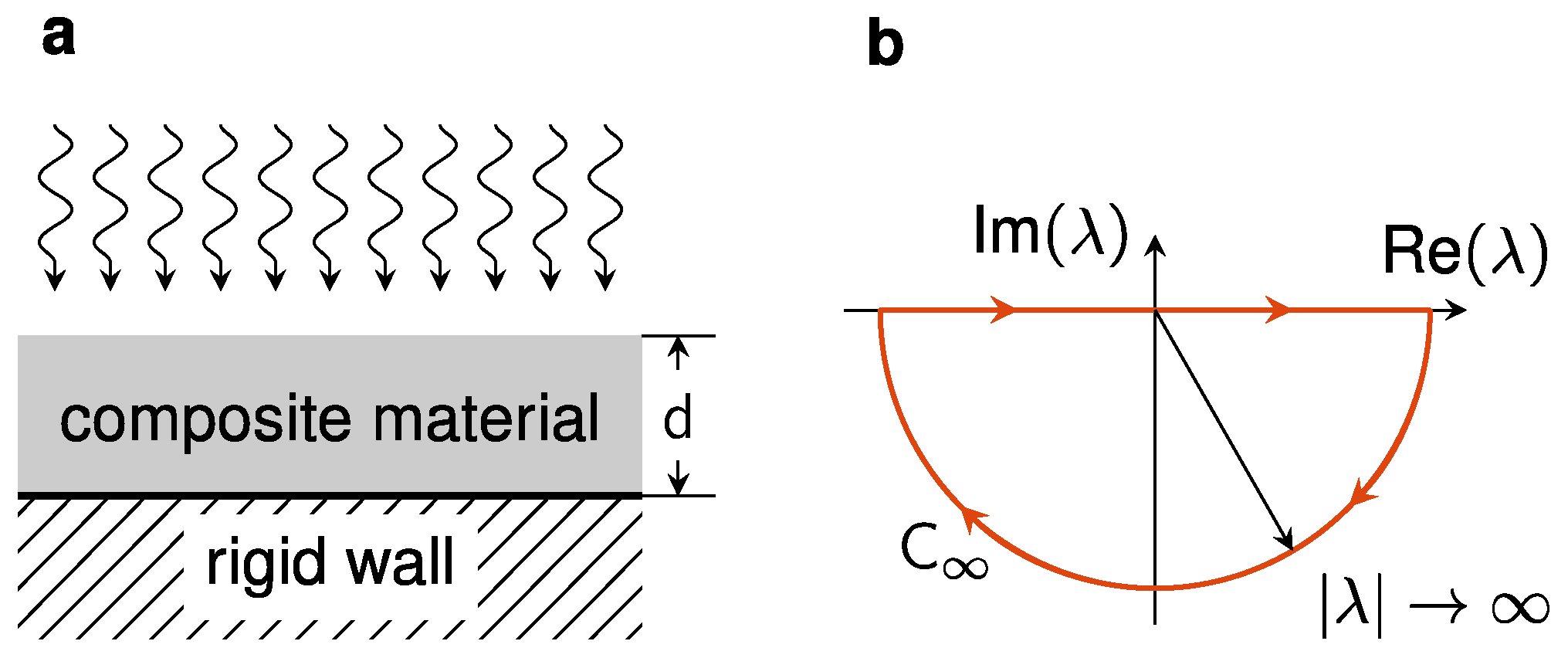
Consider a layer of composite material backed by a rigid reflective wall (Figure A1a). In response to an incident sound wave, the reflected sound pressure is the superposition of the direct reflection of the incoming sound pressure at that instant, plus those in response to the incoming sound wave at earlier time, , with . Hence,
where is the response kernel in the time domain. By carrying out Fourier transform , the reflection coefficient for each frequency may be expressed as
From Equation (A2), is an analytic function of complex in the upper half of the complex plane. In terms of the wavelength , where is the speed of sounds in air, that means has no singularities in the lower half-plane of complex , but may have zeros that represent total absorptions of incoming energy. Here, the imaginary part of reflects dissipation.
To determine the constraint on the reflection coefficient by the causality principle, we introduce an ancillary function after Fano and Rozanov [4,5],
where , satisfying , are the zeros located in the lower half-plane of complex , and stands for complex conjugation. Since has neither zeros nor poles at , is an analytic function in the lower half-plane of complex , and the Cauchy theorem is valid. That is, the integral over a closed contour in the lower half-plane of complex should yield zero, where the contour consists of the real axis of and the semi-circle that lies in the lower half-plane and has infinite radius as shown in Figure A1b. Hence
Note that at real wavelengths and is an even function of according to its definition Equation (A2). Taking the real part of Equation (A4) yields
Figure A1.
(a) Schematic for the geometry of the composite absorbing layer. (b) The contour for the integral in Equation (A4).
Figure A1.
(a) Schematic for the geometry of the composite absorbing layer. (b) The contour for the integral in Equation (A4).

To calculate the second integral on the right-hand-side of Equation (A5), we consider the infinite-wavelength limit of , i.e., the static limit. The reflection from a composite material layer can be characterized by an effective bulk modulus relating to its surface responses [12]. The surface displacement u under a pressure is therefore given by the relationship (pressure) = (effective bulk modulus) × (strain), or with being the sample thickness. The resulting surface impedance is given by with being the air impedance and the bulk modulus of air. Therefore, the reflection coefficient is given by
Since , the contour integral is therefore given by
where is the argument of complex . By taking the limit of in the above contour integral, one is essentially counting all the poles of in the lower half of the complex plane, with the imaginary part of each pole being relevant to the absorption of each resonance of the system. This is evident from the fact that in our previous work [12], it has been shown that the static limit the effective bulk modulus with being the nth resonance frequency of the system and the relevant oscillator strength defined in the main text. Hence, taking the limit of implies all the absorptions related to the resonances of the system are taken into account. In fact, for the designed structures shown in this work, if we let as defined in Equation (A19) below, then the above formula for is accurately equal to with porosity being the volume fraction of the air phase. This is in agreement with Wood’s formula for the composite effective bulk modulus in the static limit, given by . Since , follows. In addition, for samples with identical FP channels either straight or folded, where is the area of FP channels’ total surface cross sectional area and being the total area of the sample surface exposed to incident sound. Hence in this work we have .
For the third integral on the right-hand-side of Equation (A5), since , we have
Substitution of Equations (A7) and (A8) into Equation (A5) yields
As , where stands for the absorption coefficient, and all are in the lower half-plane, i.e., , we therefore have the inequality
It follows from Equation (A9) that the equality in (A10) is attained when has no zeros in the lower half-plane of complex . Such corresponds to the minimum phase-shift frequency dependence [4,5] for which the variation of the phase of the reflection coefficient with does not exceed , in the domain .
Appendix B. Inclusion of Higher Order FP Resonances in the Design Strategy
In this section we give the derivation of the design algorithm that includes all the higher order FP resonances. For a FP channel with length , its surface impedance is defined at its mouth, , by , with
For an array of FP channels with various lengths facing the incident sound wave in parallel, their total impedance is given by
where is the structure’s surface porosity (fraction of the total surface area occupied by the open mouths of the FP channels), is the 1st-order FP resonance of the nth FP resonator, the terms with stand for higher order FP resonances, and oscillator strength . It is easy to see that Equation (A11) is equivalent to Equation (7) in the main text if we take only the terms with .
In the ideal case, is continuously distributed, i.e., is a continuous variable, Equation (A11) can be converted into an integral:
where , and is the modes density of the 1st-order FP resonances. For , the real part of the integral in Equation (A12) contributes negligibly, owing to the oscillatory nature of the integrant. The imaginary part of can be accurately approximated by a delta function; hence, we have
If we omit the higher order FP resonances and consider only the term , then by recalling that , we have . Since , we have . By letting in the limit of , where , we have thus derived Equation (10) in the main text.
To include the higher order FP resonances, we recognize that the additional impedances that arise from the higher order resonances are in parallel to those arising from the 1st order FP resonances. Since now we have to deal with multiple impedances even from a single FP resonator, we would like to denote that impedance related to the 1st order FP resonance to be . In that case
Substitution of Equation (A14) into Equation (A13) and separating out the term m = 1 from the m-summation, yields an equation for ,
The value of can be obtained from Equation (A15) through iterations, based on a given target impedance . Simultaneously, Equation (A15) also expresses the fact that the target impedance at frequency is now the consequence of impedance from the order FP resonance, plus the impedance from all the higher order FP resonances, added in parallel.
For example, if the target for and divergent for , then the value of can be determined in a piecewise fashion as follows. The piecewise fashion of the result is a natural consequence (upon iteration) of the step-function nature of the target impedance. The iteration results show that in the first frequency range , in the second frequency range , in the third frequency range , in the fourth frequency range , in the fifth frequency range , etc. In each frequency interval i, i.e., for , the 1st-order FP resonance frequency distribution can be determined by Equation (14). That is, with the initial condition when the continuous variable , where denotes the total number of 1st-order FP resonances below , Equation (A14) gives . From such 1st order FP resonance frequencies one can easily determine the required lengths of the FP resonators in the design.
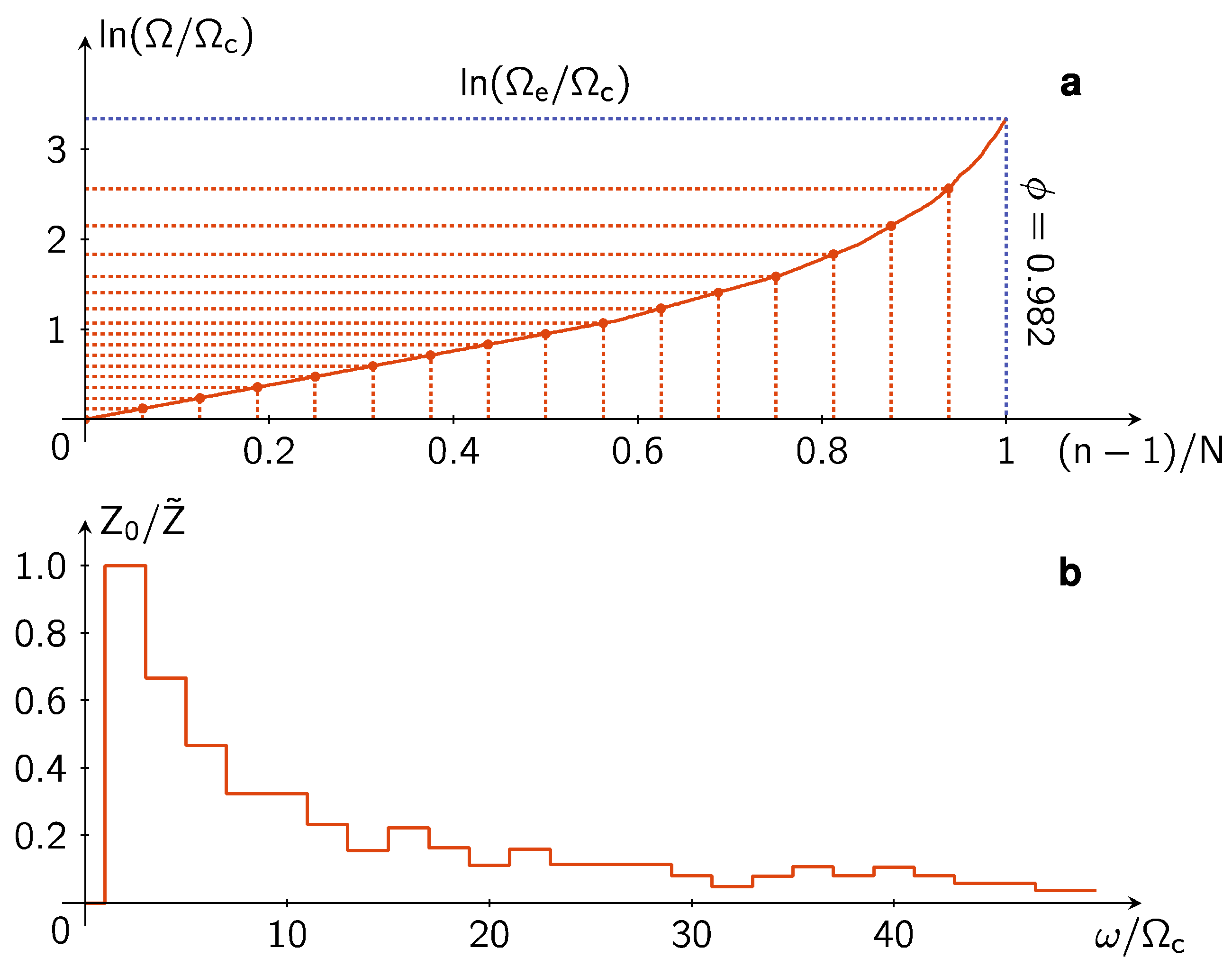
In Figure A2a we plot the natural logarithm of as a function of . Here, the value of , needed for the evaluation of , is taken to be the causally optimal value determined below. The function versus is seen to be piecewise hyper-linear. By using this result, discretization of the resonators in the actual design can be easily determined by locating the frequencies on the vertical axis with the associated (equally-spaced) values of with being the total number of FP channels one wants to use. For the broadband absorber presented in the main text with , these frequencies are explicitly indicated by the red dotted lines in Figure A2a.
One important feature for the sequence is that it decays to zero very quickly (Figure A2b), i.e., the required 1st-order FP modes density in the high frequency regime is very low. This fact is relevant to the high frequency absorption behavior for the broadband absorber presented in the main text. That is, since (this can be easily deduced from Equations (A13)–(A15)), Equation (A12) can be integrated to yield
The relevant reflection coefficient is given by
That is, at high frequencies the reflection is zero, i.e., the absorption coefficient must approach 1. Therefore, in the broadband absorber design one can use a relatively small number of FP channels, designed for the low frequencies by following the proposed recipe above, and high absorption in the high frequencies regime is guaranteed. In particular, this would ensure high absorption above 5000 Hz for the broadband absorber presented in the main text, where there are no measured data.
Figure A2.
(a) Natural logarithm of the 1st order FP resonance frequency plotted as a function of the variable as defined in the text. The discretized frequencies are picked off from the curve with equally-spaced intervals on the horizontal axis. They are indicated by the red dotted lines. (b) The iterated target impedance in Equation (A14) for the 1st-order FP resonances in the broadband absorber design, in which the contributions of higher order FP modes for each channel are taken into account. Here, is obtained from iterations through Equation (A15) based on a target impedance that is equal to above a cutoff frequency and below the cutoff. The fast decay of (to zero) guarantees that can be automatically satisfied by the higher order FP modes if the channels are designed in accordance to the recipe.

So far, the parameter remains un-determined. Below, we show that its value should not be arbitrary. Instead, it serves as the critical link between the designed mode density, the sample thickness, and the causal constraint.
In the broadband absorber, the channel length of the FP resonator is given by
provided its 1st-order resonance is located in the frequency range . Since the channel length can vary, we wish to know the minimum thickness of the sample by optimally folding the FP channels, without changing the overall area exposed to the incident wave. This minimum thickness can be obtained through volume conservation of the FP channels. Here, we evaluate by focusing on only the air channels of the FP resonators. Since the FP channels’ cross sections occupy a fraction of the surface area, is given by
where the upper limit of the integral, , is determined by the total number of 1st order mode number N, which is equal to the FP channel number. The numerical evaluation of Equation (A9), with N = 16, gives . By requiring given in the main text, we obtain the causally optimal value , with the upper limit (indicated in Figure A2a by the blue dotted line). Since in experimental implementation the value of is determined by the wall thickness in our design, such a high value of is not realizable in practice. However, a lower value of the actual is seen to only degrade the absorption somewhat, as long as the mode distribution (and hence the length of the channels) is designed in accordance with the ideal value .
As another example, other than the broadband absorber presented in the main text, we have also considered a target absorption spectrum which starts with near-perfect absorption from 345 Hz and has a notch in the frequency interval [562 Hz, 995 Hz] where the absorption is close to zero. The target impedance is given by . Based on this target impedance the impedance can be obtained from Equation (A15) through iterations. Substitution of into Equation (A14) gives the designed resonance frequencies as a function of total channel number and the parameter . The associated FP channel length can then be determined. The minimum thickness of the absorber, cm, is determined from the casual integral (A10) of the absorption spectrum shown by the dashed line in Figure 5 in the main text, which is based on the integral of Equation (A12) with . In this case the value is determined from . The experimentally measured absorption for this design, with , is presented in the main text as Figure 5 by the symbols. The result shown in Figure 5 in the main text has a 3-mm layer of sponge placed in front; the total thickness of the sample is 9.33 cm.
Appendix C. Derivation of Self-Energy Due to Cross-Channel Coupling by Evanescent Waves
Since the surface impedance of the metamaterial unit is laterally inhomogeneous, it follows that the sound pressure field , where denotes the lateral coordinate at the plane , must necessarily be inhomogeneous as well. By decomposing the pressure field as , where is the surface-averaged value, it has been shown in the main text that is only coupled to the evanescent waves that decay exponential away from . In contrast, couples to the far-field propagating modes. Therefore, the measured surface impedance should be given by with being the surface-averaged z component of the air displacement velocity. The reflection coefficient is given by .
We expand in terms of the normalized Fourier basis function , where is discretized by the condition that the area integral of over the surface of the metamaterial unit must vanish, due to the fact that the same condition applies to . That means , with :
where denotes the expansion coefficient, and . The exponential variation of means that it can couple to the z component of the air displacement velocity through Newton’s law, , so that
By multiplying both sides of Equation (A21) by and integrating over the surface of the metamaterial unit’s surface, we can solve for :
where . It should be noted that in the above, the integral of is the same as the integral of , since the integral of is zero. By substituting Equation (A22) into Equation (A20) and then interchanging the order of summation and integration, we obtain
where . Since , we can approximate by . By discretizing the 2D coordinate by its 16 values, , that denotes the center position of the FP channel, and replacing by and the integral by summation, we have:
where denotes the cross-sectional area of the FP channel, and , .
According to the definition of the Green function, at the mouth of the FP channel, we have
Substitution of Equation (A24) into Equation (A26) gives
We have rearranged the series by separating the terms involving only , since by orders of magnitude. Numerically, the last term in the bracket is also small and hence only constitutes small adjustment to the results. According to the Equation (8) in the main text, the renormalized impedance is given by . Substitution of Equation (A27) (with the term neglected) into this expression for gives
where the effective Green function can be expressed in the form of the Dyson equation with a self-energy term:
Here .
Appendix D. Absorption under Oblique Incidence
Because of the subewavelength lateral scale of the FP tubes, the acoustic absorption level at oblique incidence remains essentially flat up to 50 degrees. This is seen from the numerically simulated results shown in Figure A3. Eight scenarios with the incident angle varying from 0 to 80 degrees have been simulated. At 80 degrees incidence angle, the absorption is around 50%.
Figure A3.
The absorption coefficients under different incident angles.

References
- Cummer, S.A.; Christensen, J.; Alu, A. Controlling sound with acoustic metamaterials. Nat. Rev. Mater. 2016, 1, 16001. [Google Scholar] [CrossRef] [Green Version]
- Ma, G.; Sheng, P. Acoustic metamaterials: From local resonances to broad horizons. Sci. Adv. 2016, 2, e1501595. [Google Scholar] [CrossRef] [PubMed] [Green Version]
- Landau, L.D.; Lifshitz, E.M.; Pitaevskii, L.P. Electrodynamics of Continuous Media, 2nd ed.; Butterworth-Heinemann Ltd.: Oxford, UK, 1995; Chapter 77; Volume 8, p. 265. [Google Scholar]
- Fano, R.M. Theoretical Limitations on the Broadband Matching of Arbitrary Impedances. J. Franklin Inst. 1950, 249, 57–83. [Google Scholar] [CrossRef]
- Rozanov, K.N. Ultimate thickness to bandwidth ratio of radar absorbers. IEEE Trans. Antennas. Propag. 2000, 48, 1230–1234. [Google Scholar] [CrossRef]
- Yang, M.; Chen, S.; Fu, C.; Sheng, P. Optimal sound-absorbing structures. Mater. Horiz. 2017, 4, 673–680. [Google Scholar] [Green Version]
- Climente, A.; Torrent, D.; Sánchez-Dehesa, J. Omnidirectional broadband acoustic absorber based on metamaterials. Appl. Phys. Lett. 2012, 100, 144103. [Google Scholar] [CrossRef]
- Jiang, X.; Liang, B.; Li, R.Q.; Zou, X.Y.; Yin, L.L.; Cheng, J.C. Ultra-broadband absorption by acoustic metamaterials. Appl. Phys. Lett. 2014, 105, 243505. [Google Scholar] [CrossRef]
- Romero-García, V.; Theocharis, G.; Richoux, O.; Merkel, A.; Tournat, V.; Pagneux, V. Perfect and broadband acoustic absorption by critically coupled sub-wavelength resonators. Sci. Rep. 2016, 6, 19519. [Google Scholar] [CrossRef] [PubMed] [Green Version]
- Jiménez, N.; Groby, J.; Pagneux, V.; Romero-García, V. Iridescent Perfect Absorption in Critically-Coupled Acoustic Metamaterials Using the Transfer Matrix Method. Appl. Sci. 2017, 7, 618. [Google Scholar] [CrossRef]
- Yang, M.; Ma, G.; Yang, Z.; Sheng, P. Coupled membranes with doubly negative mass density and bulk modulus. Phys. Rev. Lett. 2013, 110, 134301. [Google Scholar] [CrossRef] [PubMed]
- Yang, M.; Ma, G.; Wu, Y.; Yang, Z.; Sheng, P. Homogenization scheme for acoustic metamaterials. Phys. Rev. B Condens. Matter Phys. 2014, 89, 064309. [Google Scholar] [CrossRef] [Green Version]
- Yang, M.; Sheng, P. Sound Absorption Structures: From Porous Media to Acoustic Metamaterials. Annu. Rev. Mater. Res. 2017, 47, 83–114. [Google Scholar] [CrossRef]
- Maa, D.-Y. Theory and design of microperforated-panel sound-absorbing construction. Sci. Sin. 1975, 18, 55–71. [Google Scholar]
- Maa, D.-Y. Potential of microperforated panel absorber. J. Acoust. Soc. Am. 1998, 104, 2861–2866. [Google Scholar] [CrossRef]
Figure 1.
(a) A plot of the normalized impedance as a function of frequency, calculated from Equation (11). Here, the imaginary part of the impedance, denoted by the blue line, is seen to decay quickly, as expected from the oscillatory nature of the integrant in Equation (8). The real part of the impedance approaches the target value in an exponential fashion. (b) The calculated absorption coefficient is seen to approach 1 in an exponential fashion. At frequencies close to the cutoff frequency, the effect of the imaginary part can be significant, but its influence decreases quickly with increasing frequency.

Figure 2.
The integration scheme can be schematically represented by the “circle of consistency”.

Figure 3.
Metamaterial unit and its features. (a) Schematics of the metamaterial unit consisting of 16 Fabry-Perot (FP) channels, arrayed in a 4 × 4 square lattice. A photo image of a sample comprising 4 units arranged in a mirror-symmetric pattern is shown in the lower left panel. (b) The surface impedance of the metamaterial unit plotted as functions of frequency. The circles are deduced from the measured reflection coefficient while the curves are the theory predictions. The arrow denotes the frequency at which the simulations were carried out on the sound pressure field, shown in the right panel below. (c) Right panel: The simulated sound pressure field at 0.22 mm above the front surface of the metamaterial unit at 612 Hz, which is the anti-resonance frequency between the FP resonances of the 5th and 6th channels (blue and red squares), shown in the left panel. The color is indicative of the pressure amplitude normalized to that of the incident wave. At anti-resonance, there is no coupling to the propagating modes; only an evanescent mode exists as explained in the text.

Figure 4.
Absorption performance of the metamaterial unit with a thin layer of acoustic sponge placed on top. Red circles are the data points measured by the impedance tube, and the red solid line is the calculated absorption by using the impedance evaluated from Equation (15). Here, the value of = 1.4. The dashed line indicates the designed cutoff frequency. Excellent agreement between theory and experiment is seen. The absorption below the cutoff frequency is largely due to the acoustic sponge.

Figure 5.
A designed absorption spectrum as indicated by the dashed line. The performance of the actual implementation with 16 FP resonators, with 3 mm of acoustic sponge on top, is shown by red circles. The red solid line is the theory prediction. It agrees very well with the experimental data as measured by the impedance tube.

Figure 6.
Reflection loss (dB) for the 5.93-cm thick designed metamaterial absorber (red curve (theory) and symbols (experiment, measured by using the impedance tube)), the micro-perforated panel (MPP) absorber with 6-cm back chamber (blue curve (theory) and symbols (experiment)), and a layer of 6-cm thick fiberglass (green symbols (experiment)). The blue curve is from Maa’s theoretical model and pentagons are the experimental data from Maa’s original paper [14,15]. It is seen that the solid red curve is about 3 to 5 dB above the red open circles, which represent the measured results. This difference is due to the fabrication error of not being able to achieve the required (very thin) thickness of the walls separating the FP channels.

© 2018 by the authors. Licensee MDPI, Basel, Switzerland. This article is an open access article distributed under the terms and conditions of the Creative Commons Attribution (CC BY) license (http://creativecommons.org/licenses/by/4.0/).
Share and Cite
MDPI and ACS Style
Yang, M.; Sheng, P. An Integration Strategy for Acoustic Metamaterials to Achieve Absorption by Design. Appl. Sci. 2018, 8, 1247. https://doi.org/10.3390/app8081247
AMA Style
Yang M, Sheng P. An Integration Strategy for Acoustic Metamaterials to Achieve Absorption by Design. Applied Sciences. 2018; 8(8):1247. https://doi.org/10.3390/app8081247
Chicago/Turabian StyleYang, Min, and Ping Sheng. 2018. "An Integration Strategy for Acoustic Metamaterials to Achieve Absorption by Design" Applied Sciences 8, no. 8: 1247. https://doi.org/10.3390/app8081247
Note that from the first issue of 2016, this journal uses article numbers instead of page numbers. See further details here.