A Review of Ghost Imaging via Sparsity Constraints

Abstract

Different from conventional imaging methods, which are based on the first-order field correlation, ghost imaging (GI) obtains the image information through high-order mutual-correlation of light fields from two paths with an object appearing in only one path. As a new optical imaging technology, GI not only provides us new capabilities beyond the conventional imaging methods, but also gives out a new viewpoint of imaging physical mechanism. It may be applied to many potential applications, such as remote sensing, snap-shot spectral imaging, thermal X-ray diffraction imaging and imaging through scattering media. In this paper, we reviewed mainly our research work of ghost imaging via sparsity constraints (GISC) and discussed the application and theory prospect of GISC concisely.

1. Introduction

With the concept of photon introduced by Albert Einstein in 1905, the statistical description of light wave is absolutely necessary for characterizing the fluctuation of light sources. Classical and quantum optical coherence theory were established by Emil Wolf in 1954 [1,2,3,4] and Roy J. Glauber in 1960 [5,6], respectively, to interpret the statistical properties of light fields. From the viewpoint of optical coherence theories, conventional imaging methods are based on the first-order correlation of light fields, and the attempt to extract spatial information of an object from high-order correlation of light fields can be traced back to the famous HBT experiment, which was conducted by R. Hanbury Brown and R. Q. Twiss in 1956 [7,8] based on the second-order autocorrelation of light fields in time domain. In 1995, Shih’s group first demonstrated a novel imaging modality, called GI [9], by correlating an output of a single-pixel (bucket) photodetector, which collected light transmitted through or reflected from an object, with an output from a high spatial-resolution scanning photodetector or photodetector array whose illumination has not interacted with the object. The physics of GI has been thoroughly discussed in the past decades [10,11,12,13,14,15,16,17]. Theories and experiments have showed that both quantum two-photon interference and classical intensity-fluctuation correlations could be used for GI. In this review, for the sake of the consistency of the discussion, we focused on the GI researches performed by our group, which is mainly based on the classical coherence theory.

The remainder of the paper is organized as follows. In Section 2, we introduce the theoretical framework of GISC with an emphasis on that the ensemble average required by GI could hardly be satisfied in real applications. In Section 3, we present a brief review of application researches of GISC conducted in Shanghai Institute of Optics & Fine Mechanics (SIOM), including two imaging applications in real space, GISC LiDAR [18,19] illuminated by pseudo-thermal light and GISC spectral camera [20] illuminated by natural light, and two imaging applications in Fourier space, X-ray Fourier-transform GISC [21] and lensless Wiener-Khinchin telescope based on high-order spatial autocorrelation of thermal light [22]. Section 4 is devoted to a discussion of the prospect of GISC.

2. Theoretical Framework of GISC

According to GI theory [10,16,17,23], we have

$$〈\Delta I_t\left(x_t\right)\Delta I_r\left(x_r\right)〉=O(x_t,x_r),$$

(1)

where $\Delta I_t\left(x_t\right)$ and $\Delta I_r\left(x_r\right)$ are intensity fluctuations of a test and a reference arms, respectively, $O(x_t,x_r)$ is a representation of an object’s image (such as an image in the real or Fourier-transform space), $〈\cdots 〉$ is the ensemble average. When the intensity in the test arm is detected by a bucket or point detector and the corresponding coordinate $x_t$ is fixed, $O(x_t,x_r)$ can be expressed as $O\left(x_r\right)$.

Since the sampling is always limited in practice, the solution of Equation (1) can be approximately presented as

$$O\left(x_r\right)\approx {\displaystyle \frac{1}{N}}\sum _{i=1}^N\Delta I_t^{\left(i\right)}\left(x_t\right)\Delta I_r^{\left(i\right)}\left(x_r\right),$$

(2)

where N is the number of samples. Many algorithms have been proposed to improve the imaging quality of GI [24,25]. In term of statistical signal processing, $O\left(x_r\right)$ corresponds to an expectation, and ${\displaystyle \frac{1}{N}}{\sum }_{i=1}^N\Delta I_t^{\left(i\right)}\left(x_t\right)\Delta I_r^{\left(i\right)}\left(x_r\right)$ denotes an estimator. To further improve the optimization results, the prior information of the object, which can be characterized as some kinds of sparsity constraints in many cases, should be applied in the image retrieval. Equation (2) can be expressed as

$$\underset{O\left(x_r\right)}{min}{\mu }_1{f}_1\left\{O\left(x_r\right)-{\displaystyle \frac{1}{N}}\sum _{i=1}^N\Delta I_t^{\left(i\right)}\left(x_t\right)\Delta I_r^{\left(i\right)}\left(x_r\right)\right\}+{\mu }_2{f}_2\left\{O\left(x_r\right)\right\},$$

(3)

where the first term is the data fidelity term, and the second term is the regularization term corresponding to the prior information of the object, ${\mu }_1$ and ${\mu }_2$ are the weight coefficients. Equation (3) is the regularized framework of GISC. At present, the data fidelity term in Equation (3) is usually approximated as [26,27,28]

$$\underset{O}{min}{\mu }_1{f}_1\left\{Y-AO\right\},$$

(4)

in a way that the existing optimization theoretical achievements such as compressive sensing (CS) [29,30,31] can be directly applied, where Y is a reshaped intensity distributions $I_t\left(x_t\right)$ in the test arm, measurement matrix A consists of the intensity distributions $I_r\left(x_r\right)$ in the reference arm. Another benefit of this approximation is that the imaging efficiency and imaging fidelity of a GI facility can be discussed in a manner of information theory [32,33]. It has been demonstrated that speckle patterns can be optimized by maximizing the mutual information between the sampling signals and the probability distribution function of the target’s images [34]. Another method to describe an image statistical prior with sparse representation is dictionary learning [35,36], and the measurement matrix optimization based on dictionary learning and the mutual coherence of the matrix, has also been demonstrated [37].

3. Applications of GISC

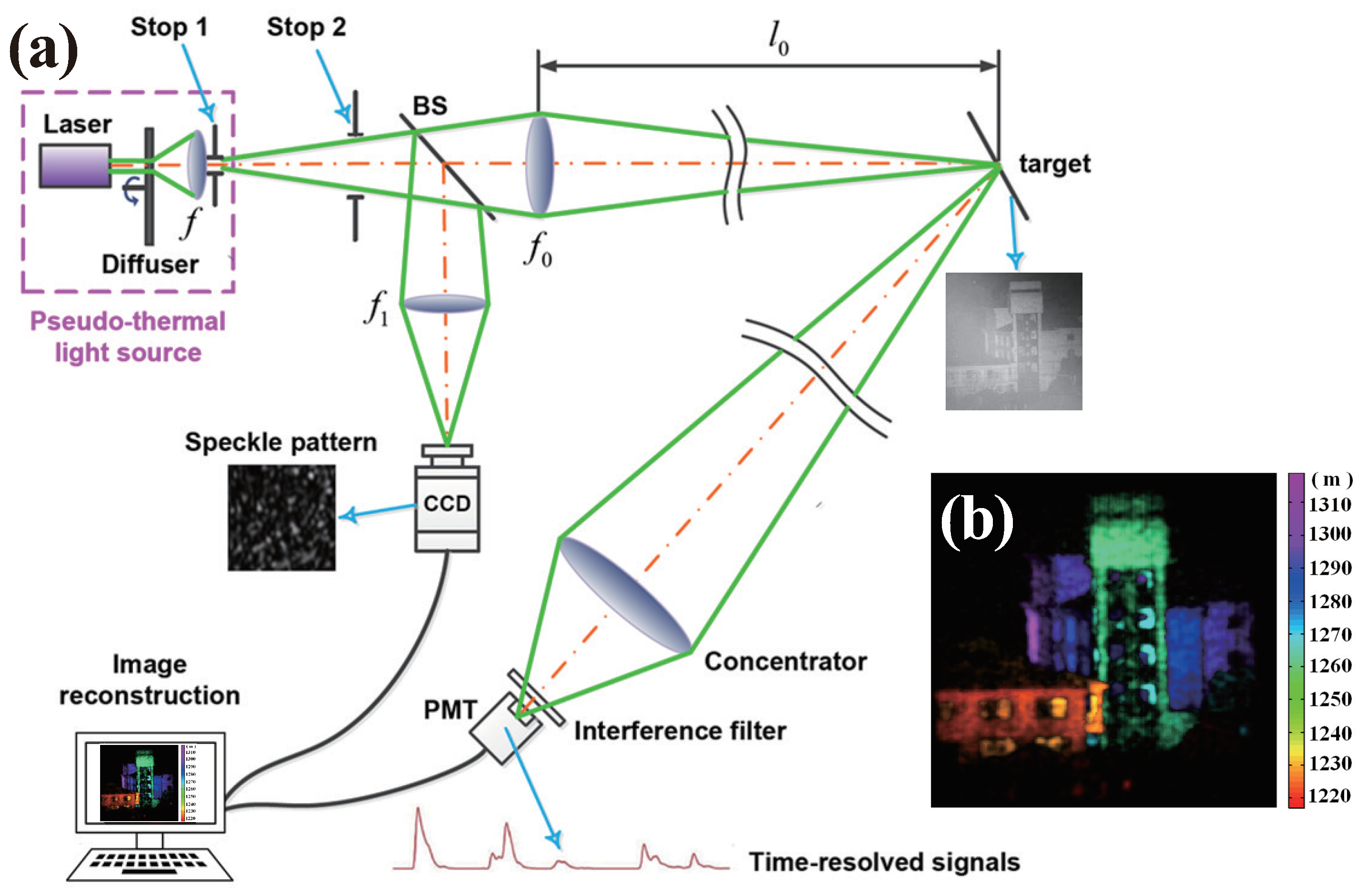
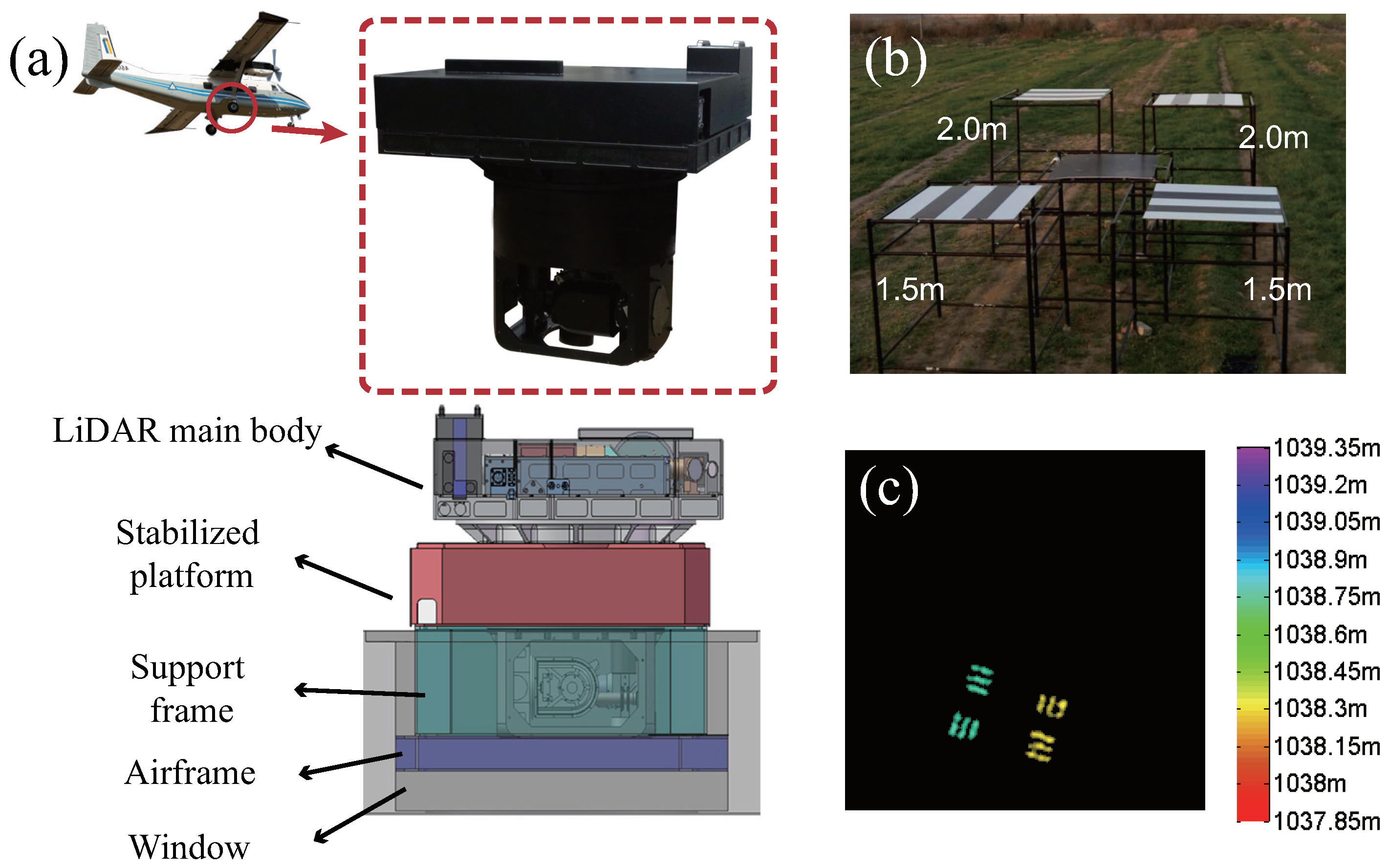
3.1. GISC LiDAR

As an important detection tool, LiDAR has been widely used in remote sensing in recent decades [38,39]. Traditional imaging LiDAR can be classified into two types: a scanning mode and a non-scanning mode (such as flash radiography) [40,41,42]. In the scanning mode, a real-space image of a target is obtained by scanning the target region point-by-point with a pulsed laser [41]. Therefore, it is difficult to image a high-speed moving target. The Non-scanning mode, characterized by an imaging system with high resolution and a pulsed flash laser, can cover the whole field of the target and obtain the real-space image in a single exposure [42]. However, because the light intensity reflected by the target is divided onto many small pixels of charge-coupled device (CCD) camera, the detection sensitivity is poor, so the detection distance of the non-scanning LiDAR is limited by the signal-to-noise ratio (SNR) of the received photons distributed on the aperture of the imaging system. Currently, it is still difficult for the traditional LiDARs to achieve high-resolution images in long ranges. In addition, all these imaging methods require sampling rate at or beyond the Nyquist limit. GISC LiDAR was proposed to obtain a high-resolution 2D or 3D image in real-space at a sampling rate significantly less than the Nyquist rate with a time-resolved single-pixel detector, which means that it has the capability of both high efficiency in information extraction and high sensitivity in detection [18,19].

Generally speaking, GISC in real-space requires that a measurement distance (between the detector and the light source) in the reference arm equals to an illuminating distance (from the light source to the target) in the test arm, and all of the reflected intensity distribution in the test arm is collected by a bucket detector. However, in remote sensing, the distance to the target, a.k.a., illumination distance, is usually unknown, so matching the measurement distance to the illuminating distance is not a reasonable option. In addition, the optical aperture in practice is very limited, so that only a small fraction of the reflected intensity from the remote target can be collected. Therefore, two key issues should be addressed in GISC LiDAR: (1) light fields on the target and the reference detection plane should be correlated, even when the test arm is far longer than the reference arm, (2) high quality images should still be reconstructed with only a small fraction of the reflected light.

The second-order longitudinal correlation length of a thermal source can be expressed as [43]

$$\Delta l_z\propto \lambda {\left(\frac{z}{D}\right)}^2$$

(5)

where $\lambda$ is the wavelength, z is the illuminating distance from the light source to the target, and D is the diameter of the pseudo-thermal light source. Researches have shown that 3D GI can still be achieved as long as the difference between the illumination and measurement distances is within the spatial longitudinal correlation length of the pseudo-thermal light source [44]. In 2009, a proof of principle experiment of far-field GI in real-space was completed [45]. According to the statistical characteristics of random speckle fields, the sum of multiple speckle intensity is proportional to the sum of total speckle intensity. The intensity correlation of light fields between the reference and test arms still holds, when the receiving aperture is not much smaller than the transmission aperture, only part of the reflected light is necessary to achieve the equivalent ‘bucket’ detection and realize 3D images in 3D GISC LiDAR [46]. These not only give a theoretical support for 3D GISC LiDAR, but also provide a system design guide.

Figure 1a presents a typical schematic of GISC LiDAR system [19]. A conjugate relationship, between the target surface and the sensitive plane of the CCD camera in the reference arm, ensures correlation properties between the intensity distributions on the corresponding target and camera planes. A pseudo-thermal light source, which consists of a pulsed laser, a diffuser such as a rotating ground-glass disk controlled by a high-precision motor, and a lens f, forms random speckle patterns on stop 1. The light emitted from the source goes through stop 2 and is subsequently divided by a beam splitter (BS) into an object and a reference paths. In the object path, the speckle pattern on stop 1 is imaged onto the target plane by an objective lens $f_0$. The photons reflected from the target are collected by a light concentrator and then passes through an interference filter into a photomultiplier tube (PMT) connected with a high-speed digitizer (an equivalent time-resolved single-pixel bucket detector). In the reference path, CCD camera is placed on an image plane of stop 1.

In 2012, GISC LiDAR was first demonstrated experimentally with a target 900 m away in real atmosphere [18]. A year later, a 3D image of a real scene at a range of approximate 1.0 km was demonstrated [19]. However, compared to the traditional nonscanning LiDAR, GISC LiDAR usually requires many measurements in a long data acquisition time to achieve the information of the object. While in remote sensing applications, either the LiDAR system is often placed on a moving platform such as an airborne craft and a vehicle, or the object is a moving target with high speed, thus the relative motion between the LiDAR system and target during sampling process will result in motion blur inevitably [47,48,49,50]. Besides algorithms and strategies that have been proposed to overcome motion blurs due to constant relative speeds [49,50], two new approaches are developed recently to further improve the imaging performance. One is to short the sampling time by either increasing the sampling speed or decreasing the number of samples. The other is to adopt the traditional motion compensation techniques to stare at the scene to be imaged during the sampling process.

A. Fast Sampling Methods

(a) Prefabricated pseudo-thermal light source. As depicted in Figure 1a, a reference CCD camera is placed in the reference path to record the intensity distributions simultaneously, and the sampling speed is constrained by the frames rate of the camera. Therefore, a prefabricated pseudo-thermal light source has been proposed to breakthrough this speed constraint. The key of the technique is to accurately address incident positions on a diffuser by a high-precision motor to produce repeatable pseudo-thermal speckle patterns. All reference intensity distributions are recorded in a low speed in advance, eliminating the camera recording in the imaging process [51,52,53].

(b) Structure 3D image reconstruction algorithms. As described above, GISC technique exploits the sparsity of a natural target as a constraint, and it can reconstruct the target with a sampling rate far below the Nyquist limit. In a 3D image reconstruction, the orthogonal properties of the target at different distances can be also used for better reconstruction. Taking these into consideration, the number of measurement required to realize a successful 3D reconstruction can be greatly reduced, which is also constructive for fast imaging [19,54].

B. Motion Compensation Techniques

Both the inertial navigation technique and the opto-electronic detection technique [55,56] are suitable for motion compensation. The inertial navigation system mainly consists of a global positioning system (GPS) and an inertial measurement unit (IMU). It makes use of the GPS information of both the LiDAR system and the target, together with the IMU information of LiDAR system, to compensate the relative motion. While the traditional opto-electronic detection technique relies on conventional thermal or visible light images of reference markers. The optimization program for motion compensation is [49]

$$X\left(\mu \right)=arg\underset{X}{min}\left|\right|y-{A\left(\mu \right)X\left|\right|}_2^2,s.t.X\ge 0,$$

(6)

with the discrepancy $D\left(\mu \right)$ between the calculated signal and the recorded data as:

$$D\left(\mu \right)=\left|\right|Y-{A\left(\mu \right)X\left(\mu \right)\left|\right|}_2^2/{\left|\right|Y\left|\right|}_2^2,$$

(7)

where $\mu$ is the unknow constant speed of the target, $A\left(\mu \right)$ is the measurement matrix dependent on the relative speed $\mu$ of the target.

With the techniques mentioned above, an airborne 3D GISC LiDAR image with 0.48 m horizontal resolution as well as 0.5 m range resolution at approximately 1.04 km height is experimentally demonstrated in 2016 [57] (Figure 2). As shown in Figure 2c, this system has the capability of motion deblurring and it realizes successful 3D reconstruction on a high-speed platform.

In the past decade, GISC LiDAR has experienced leapfrogging development from principle demonstration, static platforms and static targets to moving platforms and moving targets [19,57], and is promising to be applied in many fields such as high resolution airborne remote sensing, underwater detection and imaging, traffic monitoring, and so on. However, further theoretical and experimental researches in many aspects still need to be performed. For example, the unified theory of GISC LiDAR based on information theory and light field encoding, 1-bit compressive sensing theory [58] for GISC with photon counting detection, and the image quality evaluation of GISC LiDAR are still open questions.

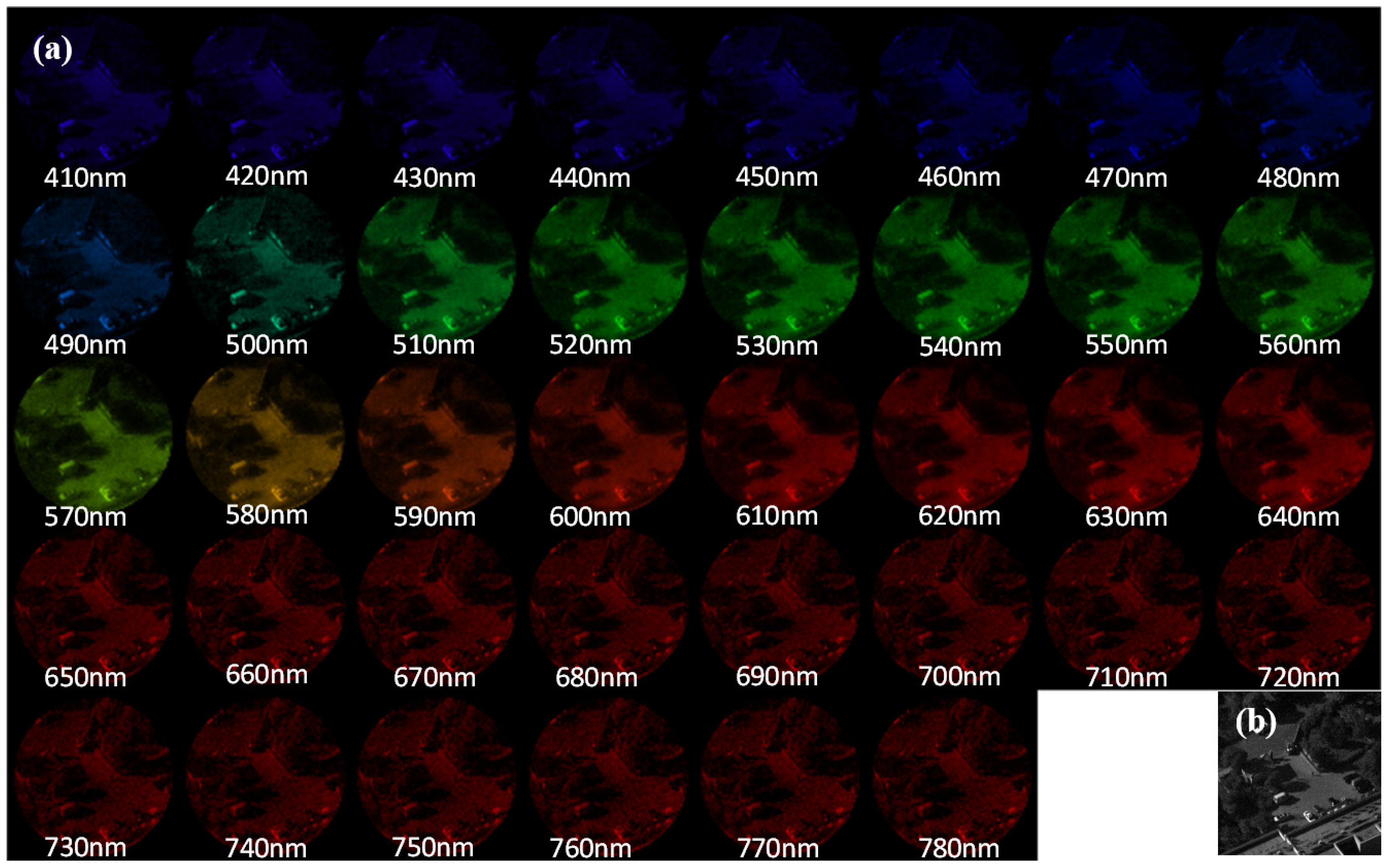
3.2. GISC Spectral Camera

Spectral imaging is a multidimensional data acquisition technology combining spectroscopic and image analysis, which captures a 3D spectral data-cube (x, y, $\lambda$) about a scene to be imaged. With both spatial and spectral resolving capabilities, it is extremely effective and vital for scene survey and detail information extraction. Conventional spectral imaging, with th point-to-point corresponding between the object and image planes, requires time-consumed scanning along either a spatial or wavelength axis since the 3D spectral data-cube is detected by a 2D detector [59]. Hence, its application is restricted in fields such as ultra-fast imaging [60,61]. Recently, remarkable snap-shot spectral imaging techniques have been widely developed to acquire a 3D spectral data-cube in just a single exposure [62,63,64,65,66]. However, since the correlation between pixels and wavelengths of the 3D image data-cube is not utilized in these methods, the information acquisition efficiency is lower than the Shannon limit [67,68]. Another important category of snapshot spectral imaging approaches is the coded aperture spectral imaging, such as the coded aperture snapshot spectral imager (CASSI), which utilizes a binary-coded mask and an equilateral prism to modulate light fields and captures a spectral image with a single shot 2D measurement [69,70,71,72]. Combining with the compressive sampling principle, it improves the sampling efficiency through the compressive sampling in photoelectric detection.

GI with true thermal light has been demonstrated by detecting the temporal fluctuation of light fields and the imaging information was obtained from the second-order correlation of light fields in time domain [73,74]. This scheme requires that the time resolution of detector is close to or less than the coherence time of light field, which may be as short as femtoseconds for true thermal light [8,20,74]. Unlike the other existing imaging methods, a GISC spectral camera modulates the image at the whole spectral band, and the true thermal light is modulated into a spatial fluctuating pseudo-thermal light field by utilizing a spatial random phase modulator. In GISC spectral camera, the spectral images of the object are obtained by the second-order spatial mutual-correlation of light fields. Therefore, high time resolution isn’t required in this scheme, and the information of the object can be acquired in a single-shot measurement. As shown in Figure 3, the GISC spectral camera consists of (1) an imaging module, which projects the image of an object on the object plane ‘a’ onto the first image plane ‘b’, (2) a spatial random phase modulator, which disperses the image with different wavelengths as a random grating and modulates the image to generate speckle patterns in plane ‘c’ [20,75,76], (3) a microscope objective, which magnifies the speckle patterns in plane ‘c’, and (4) a CCD detector recording the magnified speckle patterns.

According to the theory of the GISC spectral camera [20], the correlation function of intensity fluctuations between the spatial intensity fluctuations in the pre-determined reference arm and the test arm is

$$\begin{array}{c}\Delta G^{\left(2\right)}(r_i^{\prime },{\lambda }_l^{\prime })\hfill \\ \propto {\left\{{\left\{T_i(r_i^{\prime },k_l^{\prime })\right\}}_{r_i^{\prime }}\otimes {\left\{exp\left\{2{\left[2\pi \omega (n-1)k_l^{\prime }\right]}^2\right\}\left\{exp\left[-{\left(\frac{z_2{r}_i^{\prime }}{(z_1+z_2)\zeta }\right)}^2\right]-1\right\}\right\}}_{r_i^{\prime }}\right\}}_{k_l^{\prime }}\hfill \\ \otimes {\left\{exp\left\{-{\left[2\pi \omega (n-1)\right]}^2{k_l^{\prime }}^2\right\}\right\}}_{k_l^{\prime }},\hfill \end{array}$$

(8)

where $T_i(r_i^{\prime },{\lambda }_l^{\prime })$ is the spectral images of the object, $\omega$ and $\zeta$ are the height standard deviation and transverse correlation length of the spatial random phase modulator respectively, n is the refractive index, $k_l^{\prime }=\frac{1}{{\lambda }_l^{\prime }}$, ⊗ denotes the operation of convolution. Equation (8) specifies that the spectral images of an object can be separated from the correlation function of intensity fluctuations $\Delta G^{\left(2\right)}(r_i^{\prime },{\lambda }_l^{\prime })$, while the spatial and spectral resolution are determined by the normalized second-order correlation of light fluctuations corresponding to different pixels and wavelengths in the first image plane ‘b’. Based on this model, we set up a prototype of the GISC spectral camera. To improve the reconstruction quality with low sampling rate, the structure sparsity and low-effective-rank constraints are applied in practice [77]. Figure 4 shows the experimental results of spectral imaging for vehicles, concrete ground and trees, etc. It indicates that the prototype has the capability of snapshot spectral imaging for natural scenes.

As a new optical imaging technology, the GISC spectral camera provides a unique solution for spectral imaging of dynamic processes. This GISC imaging solution may also be expanded to other multi-dimensional information (such as polarization) acquisitions, ultra-fast measurements [60,61], and super-resolution imaging [78]. With the improvement of GISC spectral camera, we believe it can be applied not only to remote sensing, but also to the consumer market.

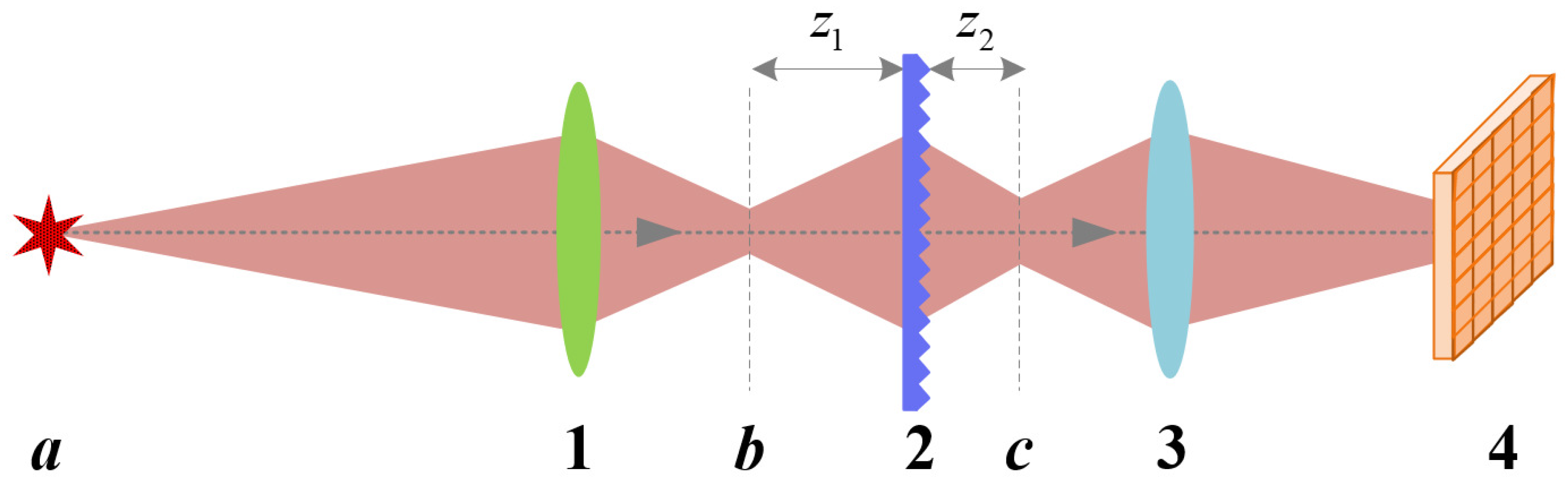
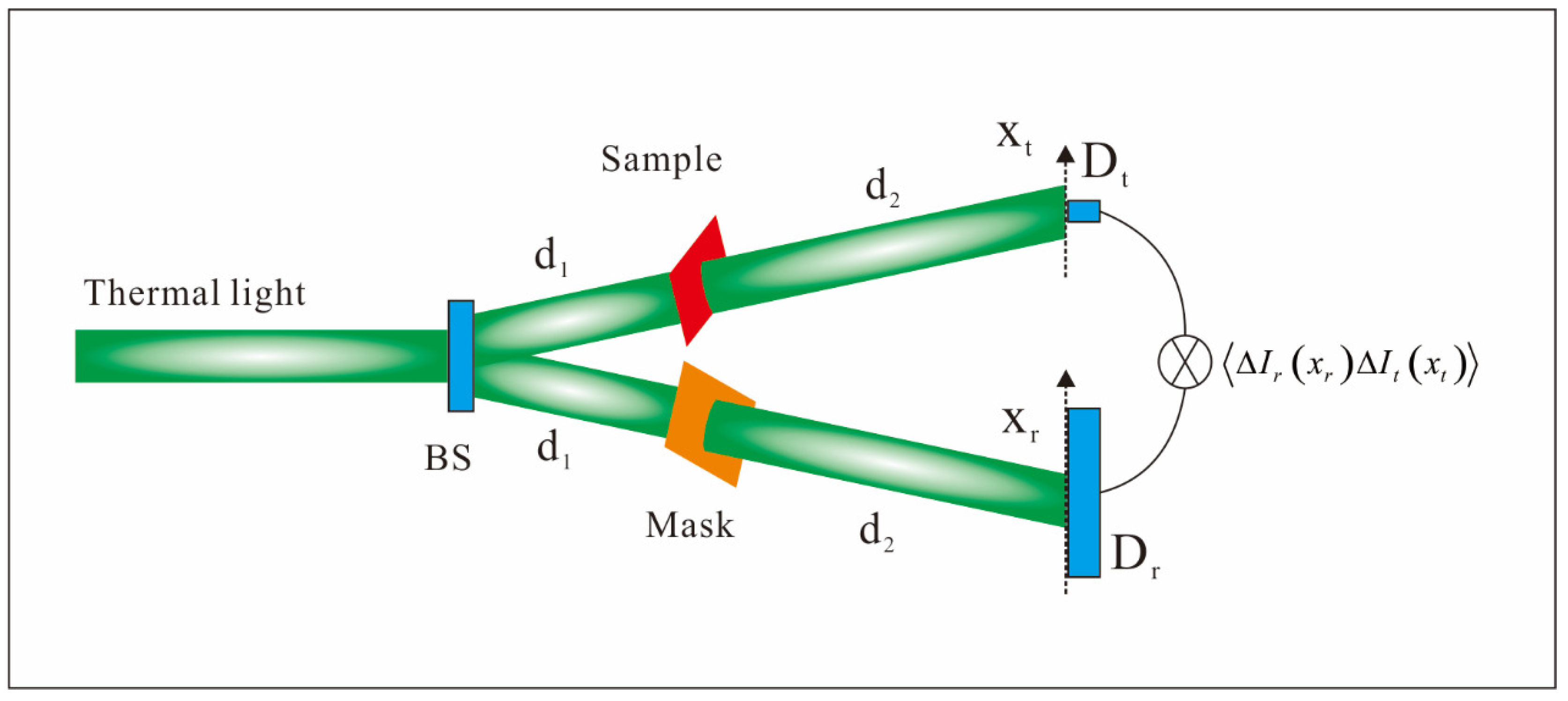
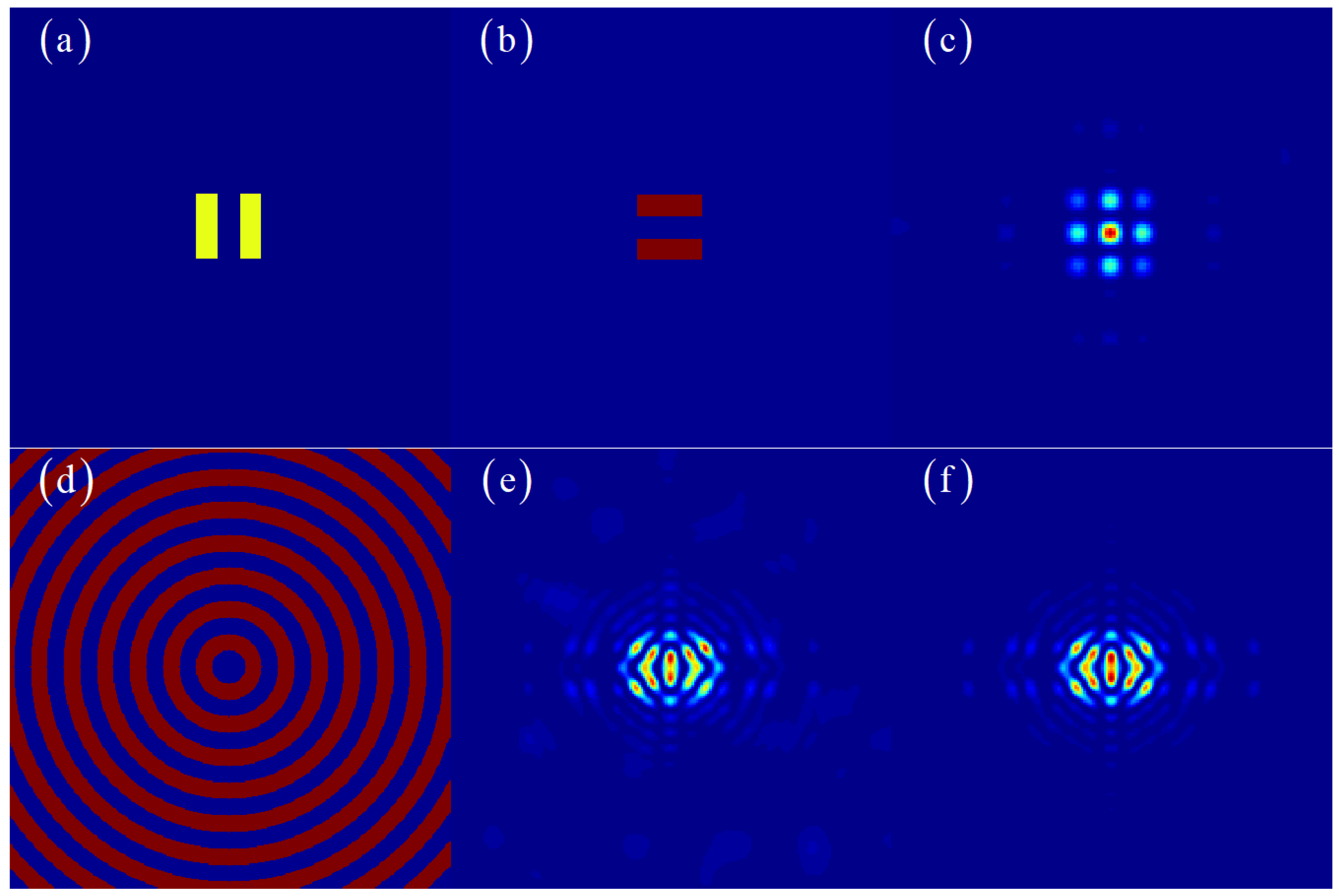
3.3. X-ray Fourier-Transform GISC

Since X-ray diffraction in crystals was discovered in 1914, X-ray crystallography has become a powerful tool in exploring and analyzing the internal structures of complex materials, such as biomolecules and nanomaterials [79,80,81]. However, the structure information of many important molecular materials, such as membrane proteins, is still out of reach, because it is difficult to grow macroscopic crystals for these materials. Meanwhile, with the rapid development of nanoscience and biology, there is an urgent need to observe the internal structures of samples in their natural states instead of in crystals. In 1999, the coherent diffraction imaging (CDI) method was proposed to extend X-ray crystallography to allow imaging noncrystalline structures in nanoscale by illuminating the samples with coherent X-rays and recording the diffraction patterns in the far field [82,83,84]. Hereafter, Fresnel CDI and ptychography techniques were proposed to circumvent the intrinsic restriction of sample size in classical CDI [85,86,87,88]. Nevertheless, the diffraction pattern within the beam stop is missing in classical CDI, and an additional technology is needed for low-frequency information. Most of all, due to the requirements for high coherence and brightness, currently, only synchrotron radiation and X-ray free electron laser sources can be used to X-ray CDI applications, and coherent imaging using laboratory X-ray sources remain unexplored.

In Fourier-transform GI (FGI), a Fourier-transform diffraction pattern of a sample can be obtained at the Fresnel region by calculating the second-order correlation of spatially incoherent light [10]. It has been demonstrated using an X-ray pseudo-thermal source [21], which provides a feasibility to achieve high-resolution microscopy with a tabletop X-ray source. Since lack of effective X-ray beam splitters, in practice the correlated light fields are generated by simply shuttling the sample in and out of the optical path between the source and the detector. In 2015, Candes group proposed a method of phase retrieval from encoded diffraction patterns to achieve better image quality in the classical CDI, where the sample is encoded by a group of random masks in real space. However, because of the destructive effect of X-ray irradiation, it is almost impossible to multiply encode the sample in the classical CDI. Fortunately, different from CDI techniques, in Fourier-transform GISC, the diffractive pattern of a sample in the testing path can be non-locally encoded by inserting modulation components in the reference path [89]. Therefore, multiple encoding of the sample can be easily realized and better image quality may be expected.

Figure 5 shows the principle of coded Fourier-transform GISC [89]. A thermal light beam is split into two paths. The sample is in the testing path and a point detector records the intensity signals of this path. In the reference path, a mask is inserted and a panel detector records the intensity distributions. The distances between the beam splitter and the detector in both paths are equal, and the mask’s position in the reference arm is the same as the sample’s position in the testing arm.

The correlation function between the intensity fluctuations of these two arms is proportional to a modulus of a convolution, which can be expressed as [90]

$$〈\Delta I_t\left(x_t\right)\Delta I_r\left(x_r\right)〉\propto {\left|\mathcal{F}\left\{s^{*}\left(x_r\right)O\left(x_r\right)\right\}\right|}^2,$$

(9)

where $s^{*}\left(x\right)$ is the conjugate of the mask’s transmission function, $\mathcal{F}$ represents a Fourier transform. Therefore, the Fourier-transform diffraction pattern of the sample encoded by the mask in real space can be obtained from the intensity correlation between the two paths. The mask in the reference path can “non-locally” encode the information of the sample in the test path. For pseudo-thermal light, it is easy to modulate the speckle fields in a predetermined manner, so we can alter the masks in the reference path to get different encoded patterns. Obviously, when $s\left(x\right)=1$, Equation (9) degenerates to the conventional Fourier diffraction pattern of the sample. Based on recombination and reutilization of the correlated intensity distributions of light fields, a spatial multiplexing reconstruction method has been proposed to improve the sampling efficiency and image quality of Fourier-transform GISC. It can greatly reduce the scale of the sensing matrix in the sensing equation, and provide the feasibility of reconstruction with just a few measurements [91].

Figure 6 shows the simulation results of an encoded X-ray Fourier-transform GISC, with a wavelength of 1 nm, distances $d_1=10$ cm and $d_2=30$ cm, respectively. The sample in the testing path is a double-slits with a separation $d_{slit}=200$ μm as shown in Figure 6a, and two masks were adopted in the simulation. The first one is the same double-slit with a ${90}^{\circ }$ rotation as shown in Figure 6b. Figure 6c is the corresponding non-locally encoded Fourier-transform GISC diffraction pattern. Clearly, it is a coherent diffraction pattern of the encoded sample. Using the second one, a concentric-circle phase mask with a period of 75 μm (Figure 6d), an encoded FGI diffraction patterns as shown in Figure 6e was obtained, which is almost the same as the encoded diffraction pattern in Figure 6f obtained from the conventional coherent diffraction imaging simulation. Then the image can be reconstructed by utilizing phase retrieval algorithms with sparsity constraints [92,93,94,95,96,97,98,99,100,101].

Figure 7 is a photograph of our tabletop X-ray GISC microscope facility. The whole system is placed in a vacuum chamber and controlled remotely. A micro-focus X-ray tube with center energy at 1.25 keV is adopted as the light source. X rays emitted from the tube is filtered to get monochromic X-rays, then passes through a pinhole array and illuminates a designed diffuser to produce high contrast X-ray speckles. A controllable pseudo-thermal X-ray source is obtained by shifting the diffuser transversely. A translation device can switch the sample and the modulation masks in and out of the beam automatically. A CCD camera with a pixel size of 15 μm is arranged in the beam to detect the X-ray intensity fluctuations.

By exploiting X-ray Fourier-transform GISC, it is of great hope to realize tabletop high-resolution 3D imaging of complex materials, such as biomolecules and nanomaterials. As a unique lensless imaging scheme, Fourier-transform GISC may also be introduced to neutron optics [102], its novel capability to image crystalline and noncrystalline samples, especially the micro magnetic structures, will bring important applications to various scientific frontiers.

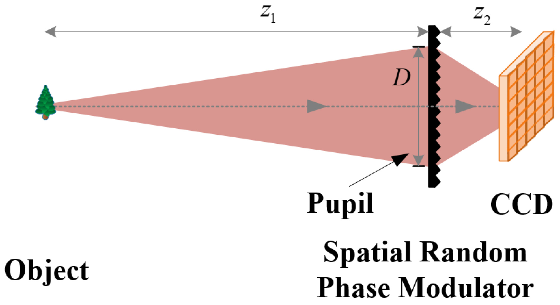
3.4. Lensless Wiener-Khinchin Telescope

Image resolution is always an important issue in various fields of scientific researches and engineering applications, many great work and discussions of resolution have been made by researchers. For conventional imaging technologies, which is based on the point-to-point correspondence between the object and the image planes, the resolution can be accurately analyzed with the transmission function of the imaging systems [103,104]. However, for imaging systems based on the wavefront random phase modulation [20,64,105,106,107,108], since the point-to-point correspondence doesn’t exist anymore, their resolution ability is difficult to be directly obtained from the transmission function, but can be obtained by analyzing the high-order correlation of light fields. Based on high-order spatial autocorrelation of thermal light, a lensless Wiener-Khinchin telescope was proposed [22]. It can acquire an image of an object in a single-shot measurement simply with a spatial random phase modulator.

As shown in Figure 8, the lensless Wiener-Khinchin telescope consists of a spatial random phase modulator and a CCD detector, whose positions are fixed. The object is illuminated by a true thermal light source.

The second-order spatial autocorrelation of the detected light is [22]

$$G_{I_t}^{\left(2\right)}\left(r+\Delta r,r\right)\propto {\left\{\left[1+g_h^{\left(2\right)}\left({\displaystyle \frac{\Delta r_0}{2\lambda z_1}}\right)\right]\otimes {\mathcal{F}}^{-1}{\left\{{\left|\mathcal{F}{\left\{I_0\left(r_0\right)\right\}}_{r_0\to f_{r_0}}\right|}^2\right\}}_{f_{r_0}\to \Delta r_0}\right\}}_{-{\displaystyle \frac{z_1}{z_2}}\Delta r},$$

(10)

where $I_0\left(r_0\right)$ is the intensity in the object plane, $r_0$ and r are the coordinates in object plane and the sensitive surface of the CCD detector, respectively. $g_h^{\left(2\right)}\left({\displaystyle \frac{\Delta r_0}{2\lambda z_1}}\right)$ is the normalized second-order correlation of the incoherent impulse response distribution. Equation (10) indicates that the Fourier transform of the intensity distribution $I_0\left(r_0\right)$ on the object plane $\left|\mathcal{F}{\left\{I_0\left(r_0\right)\right\}}_{r_0\to f_{r_0}}\right|$ can be separated from $G_{I_t}^{\left(2\right)}\left(r+\Delta r,r\right)$, and the resolution is determined by $g_h^{\left(2\right)}\left({\displaystyle \frac{\Delta r_0}{2\lambda z_1}}\right)$. The object $I_0\left(r_0\right)$ can be reconstructed by utilizing phase retrieval algorithms with sparsity constraints [92,93,94,95,96,97,98,99,100,101]. In some cases, only amplitude information of an object is interested, which can be used as a constraint to greatly improve the reconstruction quality in phase retrieval [109].

Images of two targets (a double slit and a starfish), illuminated by a xenon lamp, detected by the lensless Wiener-Khinchin telescope are shown in Figure 9. Different parameters are selected. For the double slit, $z_1=0.15$ m, $z_2=12$ mm, and for the starfish, $z_1=1$ m, $z_2=4$ mm.

Comparing with lensless CS imaging [72,105,110] and lensless GI [21,74,111], neither a measurement matrix nor a calibration process is required in lensless Wiener-Khinchin telescope, while the FOV of the lensless Wiener-Khinchin telescope is limited by the memory effect [112,113,114,115] of the system. The lensless Wiener-Khinchin telescope may have many applications, such as astronomical observation and X-rays remote sensing. Moreover, considering the scattering medium as the spatial random phase modulator, the lensless Wiener-Khinchin telescope may also open a door for a quantitatively description for imaging through scattering media [116,117,118,119,120].

4. Discussion and Future Work

Before the work of Emil Wolf [1,2,3,4], most researchers viewed the fluctuations of light as uninteresting “noise”, and the statistical methods is a “second-class” approach in Optics as pointed out by Joseph W. Goodman [121]. However, as a computational imaging technology based on high-order correlation of light, GISC not only may be applied to many applications including remote sensing, scattering imaging, and X-ray diffraction imaging, but also opens a way of combining optical imaging technology with modern information sciences to maximize the information gain. The researches of GISC are of course far from closed. In GI, both signals in the reference and the test arms are detected in one measurement. While in the present optimal estimation framework of GISC, the fidelity term is approximated by the conventional $min{f}_1\left\{Y-AO\right\}$ model, where only one signal $y_i\in Y$ is considered in one measurement once the system is calibrated. A self-consistent and more accurate optimal estimation framework for GISC, together with the developments of more powerful techniques of light field modulation, light field fluctuation detection and the electronics specially designed for GISC, are still the burning challenges to demonstrate ghost imaging applications with image quality outshine conventional imaging methods in the near future.

References

1. Wolf, E. Optics in terms of observable quantities. Il Nuovo Cim. 1954, 12, 884–888. [Google Scholar] [CrossRef]
2. Bhatia, A.B.; Wolf, E.; Born, M. On the circle polynomials of Zernike and related orthogonal sets. Math. Proc. Camb. Philos. Soc. 1954, 50, 40. [Google Scholar] [CrossRef]
3. Wolf, E. Coherence properties of partially polarized electromagnetic radiation. Il Nuovo Cim. 1959, 13, 1165–1181. [Google Scholar] [CrossRef]
4. Mandel, L.; Wolf, E. Coherence Properties of Optical Fields. Rev. Mod. Phys. 1965, 37, 231–287. [Google Scholar] [CrossRef]
5. Glauber, R.J. Photon Correlations. Phys. Rev. Lett. 1963, 10, 84–86. [Google Scholar] [CrossRef]
6. Glauber, R.J. The Quantum Theory of Optical Coherence. Phys. Rev. 1963, 130, 2529–2539. [Google Scholar] [CrossRef] [Green Version]
7. Brown, R.H.; Twiss, R.Q. Correlation between photons in two coherent beams of light. Nature 1956, 177, 27–29. [Google Scholar] [CrossRef]
8. Brown, R.H.; Twiss, R. The Question of Correlation between Photons in Coherent Light Rays. Nature 1956, 178, 1447–1448. [Google Scholar] [CrossRef]
9. Strekalov, D.V.; Sergienko, A.V.; Klyshko, D.N.; Shih, Y.H. Observation of Two-Photon “Ghost” Interference and Diffraction. Phys. Rev. Lett. 1995, 74, 3600–3603. [Google Scholar] [CrossRef] [PubMed]
10. Cheng, J.; Han, S. Incoherent coincidence imaging and its applicability in X-ray diffraction. Phys. Rev. Lett. 2004, 92, 093903. [Google Scholar] [CrossRef] [PubMed]
11. Gatti, A.; Brambilla, E.; Bache, M.; Lugiato, L.A. Ghost imaging with thermal light: Comparing entanglement and classicalcorrelation. Phys. Rev. Lett. 2004, 93, 093602. [Google Scholar] [CrossRef] [PubMed]
12. Shih, Y. The physics of ghost imaging. In Advances in Lasers and Electro Optics; Costa, N., Cartaxo, A., Eds.; InTech: Rijeka, Croatia, 2010; p. 549594. ISBN 978-953-307-088-9. [Google Scholar]
13. Kolobov, M.I. Quantum Imaging; Springer: New York, NY, USA, 2007; Volume 5, pp. 79–110. [Google Scholar]
14. Shapiro, J.H.; Boyd, R.W. The physics of ghost imaging. Quant. Inf. Process. 2012, 11, 949–993. [Google Scholar] [CrossRef] [Green Version]
15. Erkmen, B.I.; Shapiro, J.H. Ghost imaging: From quantum to classical to computational. Adv. Opt. Photonics 2010, 2, 405. [Google Scholar] [CrossRef]
16. Gong, W.; Han, S. Phase-retrieval ghost imaging of complex-valued objects. Phys. Rev. A 2010, 82. [Google Scholar] [CrossRef]
17. Song, X.B.; Xu, D.Q.; Wang, H.B.; Xiong, J.; Zhang, X.; Cao, D.Z.; Wang, K. Experimental observation of one-dimensional quantum holographic imaging. Appl. Phys. Lett. 2013, 103, 131111. [Google Scholar] [CrossRef] [Green Version]
18. Zhao, C.; Gong, W.; Chen, M.; Li, E.; Wang, H.; Xu, W.; Han, S. Ghost imaging lidar via sparsity constraints. Appl. Phys. Lett. 2012, 101, 141123. [Google Scholar] [CrossRef] [Green Version]
19. Gong, W.; Zhao, C.; Yu, H.; Chen, M.; Xu, W.; Han, S. Three-dimensional ghost imaging lidar via sparsity constraint. Sci. Rep. 2016, 6. [Google Scholar] [CrossRef] [PubMed]
20. Liu, Z.; Tan, S.; Wu, J.; Li, E.; Shen, X.; Han, S. Spectral camera based on ghost imaging via sparsity constraints. Sci. Rep. 2016, 6. [Google Scholar] [CrossRef] [PubMed]
21. Yu, H.; Lu, R.; Han, S.; Xie, H.; Du, G.; Xiao, T.; Zhu, D. Fourier-transform ghost imaging with hard X rays. Phys. Rev. Lett. 2016, 117, 113901. [Google Scholar] [CrossRef] [PubMed]
22. Liu, Z.; Shen, X.; Liu, H.; Yu, H.; Han, S. Lensless Wiener-Khinchin telescope based on high-order spatial autocorrelation of thermal light. arXiv, 2018; arXiv:1804.01270v4. [Google Scholar]
23. Valencia, A.; Scarcelli, G.; D’Angelo, M.; Shih, Y. Two-Photon Imaging with Thermal Light. Phys. Rev. Lett. 2005, 94. [Google Scholar] [CrossRef] [PubMed] [Green Version]
24. Gong, W.; Han, S. A method to improve the visibility of ghost images obtained by thermal light. Phys. Lett. A 2010, 374, 1005–1008. [Google Scholar] [CrossRef]
25. Ferri, F.; Magatti, D.; Lugiato, L.; Gatti, A. Differential ghost imaging. Phys. Rev. Lett. 2010, 104, 253603. [Google Scholar] [CrossRef] [PubMed]
26. Katz, O.; Bromberg, Y.; Silberberg, Y. Compressive ghost imaging. Appl. Phys. Lett. 2009, 95, 131110. [Google Scholar] [CrossRef] [Green Version]
27. Wang, H.; Han, S.; Kolobov, M.I. Quantum limits of super-resolution of optical sparse objects via sparsity constraint. Opt. Express 2012, 20, 23235. [Google Scholar] [CrossRef] [PubMed]
28. Wang, H.; Han, S. Coherent Ghost Imaging based on sparsity constraint without phase-sensitive detection. Europhys. Lett. 2012, 98, 24003. [Google Scholar] [CrossRef]
29. Donoho, D.L. Compressed sensing. IEEE Trans. Inf. Theory 2006, 52, 1289–1306. [Google Scholar] [CrossRef]
30. Candès, E.J.; Romberg, J.; Tao, T. Robust uncertainty principles: Exact signal reconstruction from highly incomplete frequency information. IEEE Trans. Inf. Theory 2006, 52, 489–509. [Google Scholar] [CrossRef]
31. Eldar, Y.C.; Kutyniok, G. Compressed Sensing: Theory and Applications; Cambridge University Press: Cambridge, UK, 2012. [Google Scholar]
32. Li, J.; Luo, B.; Yang, D.; Yin, L.; Wu, G.; Guo, H. Negative exponential behavior of image mutual information for pseudo-thermal light ghost imaging: observation, modeling, and verification. Sci. Bull. 2017, 62, 717–723. [Google Scholar] [CrossRef] [Green Version]
33. Akçakaya, M.; Tarokh, V. Shannon-theoretic limits on noisy compressive sampling. IEEE Trans. Inf. Theory 2010, 56, 492–504. [Google Scholar] [CrossRef]
34. Li, E.; Chen, M.; Gong, W.; Yu, H.; Han, S. Mutual information of ghost imaging systems. Acta Opt. Sin. 2013, 33, 1211003. [Google Scholar]
35. Olshausen, B.A.; Field, D.J. Natural image statistics and efficient coding. Netw. Comput. Neural Syst. 1996, 7, 333–339. [Google Scholar] [CrossRef] [Green Version]
36. Aharon, M.; Elad, M.; Bruckstein, A. $rm K$-SVD: An Algorithm for Designing Overcomplete Dictionaries for Sparse Representation. IEEE Trans. Signal Process. 2006, 54, 4311–4322. [Google Scholar] [CrossRef]
37. Hu, C.; Wang, J.; Huang, Z.; Tong, Z.; Liu, S.; Ma, S.; Liu, Z.; Han, S. Optimization of light field fluctuation patterns in ghost imaging by mutual coherence minimization based on dictionary learning. In Proceedings of the OSA Computational Optical Sensing and Imaging Conference, Orlando, FL, USA, 25–28 June 2018. [Google Scholar]
38. Yun, J.Y.J.; Gao, C.G.C.; Zhu, S.Z.S.; Sun, C.S.C.; He, H.H.H.; Feng, L.F.L.; Dong, L.D.L.; Niu, L.N.L. High-peak-power, single-mode, nanosecond pulsed, all-fiber laser for high resolution 3D imaging LIDAR system. Chin. Opt. Lett. 2012, 10, 121402–121404. [Google Scholar] [CrossRef] [Green Version]
39. Albota, M.A.; Aull, B.F.; Fouche, D.G.; Heinrichs, R.M.; Kocher, D.G.; Marino, R.M.; Mooney, J.G.; Newbury, N.R.; Player, B.E.; Willard, B.C. Three-dimensional imaging laser radars with Geiger-mode avalanche photodiode arrays. Lincoln Lab. J. 2002, 13, 351–370. [Google Scholar]
40. Elachi, C. Spaceborne Radar Remote Sensing: Applications and Techniques; IEEE Press: New York, NY, USA, 1988; 285p. [Google Scholar]
41. Ahola, R.; Heikkinen, T.; Manninen, M. 3D image acquisition by scanning time of flight measurements. In Proceedings of the International Conference on Advances in Image Processing and Pattern Recognition, Pisa, Italy, 10–12 December 1985. [Google Scholar]
42. Anthes, J.P.; Garcia, P.; Pierce, J.T.; Dressendorfer, P.V. Nonscanned ladar imaging and applications. In Applied Laser Radar Technology; Kamerman, G.W., Keicher, W.E., Eds.; SPIE: Orlando, FL, USA, 1993. [Google Scholar] [CrossRef]
43. Liu, H.; Han, S. Spatial longitudinal coherence length of a thermal source and its influence on lensless ghost imaging. Opt. Lett. 2008, 33, 824. [Google Scholar] [CrossRef] [PubMed]
44. Gong, W.; Han, S. The influence of axial correlation depth of light field on lensless ghost imaging. JOSA B 2010, 27, 675–678. [Google Scholar] [CrossRef]
45. Gong, W.; Zhang, P.; Shen, X.; Han, S. Ghost “pinhole” imaging in Fraunhofer region. Appl. Phys. Lett. 2009, 95, 071110. [Google Scholar] [CrossRef] [Green Version]
46. Han, S.; Gong, W.; Chen, M.; Li, E.; Bo, Z.; Li, W.; Zhang, H.; Gao, X.; Deng, C.; Mei, X.; et al. Research progress of GISC lidar. Infrared Laser Eng. 2015, 44, 2547–2555. [Google Scholar]
47. Li, H.; Xiong, J.; Zeng, G. Lensless ghost imaging for moving objects. Opt. Eng. 2011, 50, 127005. [Google Scholar] [CrossRef]
48. Cong, Z.; Wenlin, G.; Han, S. Ghost imaging for moving targets and its application in remote sensing. Chin. J. Lasers 2012, 12, 039. [Google Scholar]
49. Li, E.; Bo, Z.; Chen, M.; Gong, W.; Han, S. Ghost imaging of a moving target with an unknown constant speed. Appl. Phys. Lett. 2014, 104, 251120. [Google Scholar] [CrossRef]
50. Li, X.; Deng, C.; Chen, M.; Gong, W.; Han, S. Ghost imaging for an axially moving target with an unknown constant speed. Photonics Res. 2015, 3, 153–157. [Google Scholar] [CrossRef]
51. Jia, J.; Chengqiang, Z.; Lijun, C. Research on the repeatable pseudo-thermal light based on random phase plate scanning. Acta Opt. Sin. 2013, 33, 0911002. [Google Scholar] [CrossRef]
52. Nan, W.; Wenlin, G.; Shensheng, H. Experimental research on pseudo-thermal light ghost imaging with random phase plate based on variable motion trail. Acta Opt. Sin. 2015, 35, 0711005. [Google Scholar] [CrossRef]
53. Mei, X.; Gong, W.; Yan, Y.; Han, S.; Cao, Q. Experimental research on prebuilt three-dimensional imaging lidar. Chin. J. Lasers 2016, 43, 0710003. [Google Scholar]
54. Yu, H.; Li, E.; Gong, W.; Han, S. Structured image reconstruction for three-dimensional ghost imaging lidar. Opt. Express 2015, 23, 14541. [Google Scholar] [CrossRef] [PubMed]
55. Farrell, J.; Barth, M. The Global Positioning System and Inertial Navigation; McGraw-Hill: New York, NY, USA, 1999; Volume 61, pp. 1–20. [Google Scholar]
56. Masten, M.K. Inertially stabilized platforms for optical imaging systems. IEEE Control Syst. 2008, 28, 47–64. [Google Scholar]
57. Wang, C.; Mei, X.; Pan, L.; Wang, P.; Li, W.; Gao, X.; Bo, Z.; Chen, M.; Gong, W.; Han, S. Airborne Near Infrared Three-Dimensional Ghost Imaging LiDAR via Sparsity Constraint. Remote Sens. 2018, 10, 732. [Google Scholar] [CrossRef]
58. Boufounos, P.T.; Baraniuk, R.G. 1-bit compressive sensing. In Proceedings of the 42nd Annual Conference on IEEE Information Sciences and Systems, Princeton, NJ, USA, 19–21 March 2008; pp. 16–21. [Google Scholar]
59. Herrala, E.; Okkonen, J.T.; Hyvarinen, T.S.; Aikio, M.; Lammasniemi, J. Imaging spectrometer for process industry applications. In Optical Measurements and Sensors for the Process Industries; Gorecki, C., Preater, R.W.T., Eds.; SPIE: Kailua, Kona, HI, USA, 1994. [Google Scholar] [CrossRef]
60. Gao, L.; Liang, J.; Li, C.; Wang, L.V. Single-shot compressed ultrafast photography at one hundred billion frames per second. Nature 2014, 516, 74–77. [Google Scholar] [CrossRef] [PubMed]
61. Nakagawa, K.; Iwasaki, A.; Oishi, Y.; Horisaki, R.; Tsukamoto, A.; Nakamura, A.; Hirosawa, K.; Liao, H.; Ushida, T.; Goda, K.; et al. Sequentially timed all-optical mapping photography (STAMP). Nat. Photonics 2014, 8, 695–700. [Google Scholar] [CrossRef]
62. Hagen, N.; Kudenov, M.W. Review of snapshot spectral imaging technologies. Opt. Eng. 2013, 52, 090901. [Google Scholar] [CrossRef] [Green Version]
63. Gao, L.; Wang, L.V. A review of snapshot multidimensional optical imaging: measuring photon tags in parallel. Phys. Rep. 2016, 616, 1–37. [Google Scholar] [CrossRef] [PubMed]
64. Sahoo, S.K.; Tang, D.; Dang, C. Single-shot multispectral imaging with a monochromatic camera. Optica 2017, 4, 1209. [Google Scholar] [CrossRef] [Green Version]
65. Gao, L.; Kester, R.T.; Tkaczyk, T.S. Compact Image Slicing Spectrometer (ISS) for hyperspectral fluorescence microscopy. Opt. Express 2009, 17, 12293. [Google Scholar] [CrossRef] [PubMed]
66. Kudenov, M.W. Faceted grating prism for a computed tomographic imaging spectrometer. Opt. Eng. 2012, 51, 044002. [Google Scholar] [CrossRef]
67. Cover, T.M.; Thomas, J.A. Elements of Information Theory; John Wiley & Sons: New York, NY, USA, 2012; pp. 657–687. [Google Scholar]
68. Shannon, C.E. A Mathematical Theory of Communication. Bell Syst. Tech. J. 1948, 27, 379–423. [Google Scholar] [CrossRef]
69. Wagadarikar, A.A.; Pitsianis, N.P.; Sun, X.; Brady, D.J. Spectral image estimation for coded aperture snapshot spectral imagers. Proc. SPIE 2008, 7076, 707602. [Google Scholar] [Green Version]
70. Wagadarikar, A.; John, R.; Willett, R.; Brady, D. Single disperser design for coded aperture snapshot spectral imaging. Appl. Opt. 2008, 47, B44–B51. [Google Scholar] [CrossRef] [PubMed]
71. Arce, G.R.; Brady, D.J.; Carin, L.; Arguello, H.; Kittle, D.S. Compressive Coded Aperture Spectral Imaging: An Introduction. IEEE Signal Process. Mag. 2014, 31, 105–115. [Google Scholar] [CrossRef]
72. Asif, M.S.; Ayremlou, A.; Sankaranarayanan, A.; Veeraraghavan, A.; Baraniuk, R.G. FlatCam: Thin, Lensless Cameras Using Coded Aperture and Computation. IEEE Trans. Comput. Imaging 2017, 3, 384–397. [Google Scholar] [CrossRef]
73. Zhang, D.; Zhai, Y.H.; Wu, L.A.; Chen, X.H. Correlated two-photon imaging with true thermal light. Opt. Lett. 2005, 30, 2354–2356. [Google Scholar] [CrossRef] [PubMed]
74. Liu, X.F.; Chen, X.H.; Yao, X.R.; Yu, W.K.; Zhai, G.J.; Wu, L.A. Lensless ghost imaging with sunlight. Opt. Lett. 2014, 39, 2314–2317. [Google Scholar] [CrossRef] [PubMed]
75. Giglio, M.; Carpineti, M.; Vailati, A. Space intensity correlations in the near field of the scattered light: A direct measurement of the density correlation function g (r). Phys. Rev. Lett. 2000, 85, 1416. [Google Scholar] [CrossRef] [PubMed]
76. Cerbino, R.; Peverini, L.; Potenza, M.A.C.; Robert, A.; Bösecke, P.; Giglio, M. X-ray-scattering information obtained from near-field speckle. Nat. Phys. 2008, 4, 238–243. [Google Scholar] [CrossRef]
77. Liu, Z.; Tan, S.; Wu, J.; Li, E.; Han, S. The Study of Spectral Camera based on Ghost Imaging via Sparsity Constraints with Sunlight Illumination. In Proceedings of the Conference on Lasers and Electro-Optics, San Jose, CA, USA, 5–10 June 2016. [Google Scholar]
78. Tong, Z.; Wang, J.; Huang, Z.; Liu, Z.; Hu, C.; Wu, J.; Li, E.; Shen, X.; Han, S. Super-Resolution Imaging Based on Spectral Dimensional Information. In Proceedings of the OSA Computational Optical Sensing and Imaging Conference, Orlando, FL, USA, 25–28 June 2018. [Google Scholar]
79. Shi, Y. A Glimpse of Structural Biology through X-Ray Crystallography. Cell 2014, 159, 995–1014. [Google Scholar] [CrossRef] [PubMed]
80. Fleury, B.; Cortes-Huerto, R.; Taché, O.; Testard, F.; Menguy, N.; Spalla, O. Gold Nanoparticle Internal Structure and Symmetry Probed by Unified Small-Angle X-ray Scattering and X-ray Diffraction Coupled with Molecular Dynamics Analysis. Nano Lett. 2015, 15, 6088–6094. [Google Scholar] [CrossRef] [PubMed]
81. Kosynkin, D.V.; Higginbotham, A.L.; Sinitskii, A.; Lomeda, J.R.; Dimiev, A.; Price, B.K.; Tour, J.M. Longitudinal unzipping of carbon nanotubes to form graphene nanoribbons. Nature 2009, 458, 872–876. [Google Scholar] [CrossRef] [PubMed] [Green Version]
82. Miao, J.; Charalambous, P.; Kirz, J.; Sayre, D. Extending the methodology of X-ray crystallography to allow imaging of micrometre-sized non-crystalline specimens. Nature 1999, 400, 342–344. [Google Scholar] [CrossRef]
83. Chapman, H.N.; Barty, A.; Bogan, M.J.; Boutet, S.; Frank, M.; Hau-Riege, S.P.; Marchesini, S.; Woods, B.W.; Bajt, S.; Benner, W.H.; et al. Femtosecond diffractive imaging with a soft-X-ray free-electron laser. Nat. Phys. 2006, 2, 839–843. [Google Scholar] [CrossRef] [Green Version]
84. Pfeifer, M.A.; Williams, G.J.; Vartanyants, I.A.; Harder, R.; Robinson, I.K. Three-dimensional mapping of a deformation field inside a nanocrystal. Nature 2006, 442, 63–66. [Google Scholar] [CrossRef] [PubMed] [Green Version]
85. Williams, G.J.; Quiney, H.M.; Dhal, B.B.; Tran, C.Q.; Nugent, K.A.; Peele, A.G.; Paterson, D.; de Jonge, M.D. Fresnel Coherent Diffractive Imaging. Phys. Rev. Lett. 2006, 97. [Google Scholar] [CrossRef] [PubMed]
86. Abbey, B.; Nugent, K.A.; Williams, G.J.; Clark, J.N.; Peele, A.G.; Pfeifer, M.A.; de Jonge, M.; McNulty, I. Keyhole coherent diffractive imaging. Nat. Phys. 2008, 4, 394–398. [Google Scholar] [CrossRef] [Green Version]
87. Rodenburg, J.; Hurst, A.; Cullis, A.; Dobson, B.; Pfeiffer, F.; Bunk, O.; David, C.; Jefimovs, K.; Johnson, I. Hard-x-ray lensless imaging of extended objects. Phys. Rev. Lett. 2007, 98, 034801. [Google Scholar] [CrossRef] [PubMed]
88. Thibault, P.; Dierolf, M.; Menzel, A.; Bunk, O.; David, C.; Pfeiffer, F. High-Resolution Scanning X-ray Diffraction Microscopy. Science 2008, 321, 379–382. [Google Scholar] [CrossRef] [PubMed]
89. Yu, H.; Lu, R.; Tan, Z.; Zhu, R.; Han, S. X-ray Fourier-transform Ghost Imaging via Sparsity Constraints. In Proceedings of the IEEE NSS-MIC Conference, Atlanta, GA, USA, 21–28 October 2017. [Google Scholar]
90. Zhang, M. Experimental Investigation on Non-Local Lensless Fourier-Transform Imaging With Classical Incoherent Light. Ph.D. Thesis, Shanghai Institute of Optics & Fine Mechanics, Chinese Academy of Sciences, Shanghai, China, 2007. [Google Scholar]
91. Zhu, R.; Yu, H.; Lu, R.; Tan, Z.; Han, S. Spatial multiplexing reconstruction for Fourier-transform ghost imaging via sparsity constraints. Opt. Express 2018, 26, 2181. [Google Scholar] [CrossRef] [PubMed]
92. Fienup, J.R. Reconstruction of an object from the modulus of its Fourier transform. Opt. Lett. 1978, 3, 27–29. [Google Scholar] [CrossRef] [PubMed]
93. Fienup, J.R. Phase retrieval algorithms: a comparison. Appl. Opt. 1982, 21, 2758–2769. [Google Scholar] [CrossRef] [PubMed]
94. Candès, E.J.; Strohmer, T.; Voroninski, V. PhaseLift: Exact and Stable Signal Recovery from Magnitude Measurements via Convex Programming. Commun. Pure Appl. Math. 2012, 66, 1241–1274. [Google Scholar] [CrossRef] [Green Version]
95. Liu, X.; Wu, J.; He, W.; Liao, M.; Zhang, C.; Peng, X. Vulnerability to ciphertext-only attack of optical encryption scheme based on double random phase encoding. Opt. Express 2015, 23, 18955. [Google Scholar] [CrossRef] [PubMed]
96. Chen, Y.; Candes, E. Solving Random Quadratic Systems of Equations Is Nearly as Easy as Solving Linear Systems. In Advances in Neural Information Processing Systems 28; Cortes, C., Lawrence, N.D., Lee, D.D., Sugiyama, M., Garnett, R., Eds.; Curran Associates, Inc.: Montréal, QC, Canada, 2015; pp. 739–747. [Google Scholar]
97. Shechtman, Y.; Eldar, Y.C.; Cohen, O.; Chapman, H.N.; Miao, J.; Segev, M. Phase retrieval with application to optical imaging: a contemporary overview. IEEE Signal Process. Mag. 2015, 32, 87–109. [Google Scholar] [CrossRef]
98. Candès, E.J.; Eldar, Y.C.; Strohmer, T.; Voroninski, V. Phase Retrieval via Matrix Completion. SIAM Rev. 2015, 57, 225–251. [Google Scholar] [CrossRef] [Green Version]
99. Candes, E.J.; Li, X.; Soltanolkotabi, M. Phase retrieval via Wirtinger flow: Theory and algorithms. IEEE Trans. Inf. Theory 2015, 61, 1985–2007. [Google Scholar] [CrossRef]
100. Candes, E.J.; Li, X.; Soltanolkotabi, M. Phase retrieval from coded diffraction patterns. Appl. Comput. Harmonic Anal. 2015, 39, 277–299. [Google Scholar] [CrossRef] [Green Version]
101. Jaganathan, K.; Oymak, S.; Hassibi, B. Sparse Phase Retrieval: Uniqueness Guarantees and Recovery Algorithms. IEEE Trans. Signal Process. 2017, 65, 2402–2410. [Google Scholar] [CrossRef]
102. Chen, K.; Han, S. Microscopy for Atomic and Magnetic Structures Based on Thermal Neutron Fourier-transform Ghost Imaging. arXiv, 2018; arXiv:1801.10046. [Google Scholar]
103. Sheppard, C.J. Resolution and super-resolution. Microsc. Res. Tech. 2017, 80, 590–598. [Google Scholar] [CrossRef] [PubMed]
104. Baker, S.; Kanade, T. Limits on super-resolution and how to break them. IEEE Trans. Pattern Anal. Mach. Intell. 2002, 24, 1167–1183. [Google Scholar] [CrossRef] [Green Version]
105. Antipa, N.; Kuo, G.; Heckel, R.; Mildenhall, B.; Bostan, E.; Ng, R.; Waller, L. DiffuserCam: lensless single-exposure 3D imaging. Optica 2017, 5, 1. [Google Scholar] [CrossRef]
106. Adams, J.K.; Boominathan, V.; Avants, B.W.; Vercosa, D.G.; Ye, F.; Baraniuk, R.G.; Robinson, J.T.; Veeraraghavan, A. Single-frame 3D fluorescence microscopy with ultraminiature lensless FlatScope. Sci. Adv. 2017, 3, e1701548. [Google Scholar] [CrossRef] [PubMed]
107. Mukherjee, S.; Vijayakumar, A.; Kumar, M.; Rosen, J. 3D Imaging through Scatterers with Interferenceless Optical System. Sci. Rep. 2018, 8. [Google Scholar] [CrossRef] [PubMed]
108. Wang, P.; Menon, R. Ultra-high-sensitivity color imaging via a transparent diffractive-filter array and computational optics. Optica 2015, 2, 933. [Google Scholar] [CrossRef]
109. Ying, G.; Wei, Q.; Shen, X.; Han, S. A two-step phase-retrieval method in Fourier-transform ghost imaging. Opt. Commun. 2008, 281, 5130–5132. [Google Scholar] [CrossRef]
110. Huang, G.; Jiang, H.; Matthews, K.; Wilford, P. Lensless imaging by compressive sensing. In Proceedings of the 2013 IEEE International Conference on Image Processing, Melbourne, VIC, Australia, 15–18 September 2013. [Google Scholar]
111. Chen, X.H.; Liu, Q.; Luo, K.H.; Wu, L.A. Lensless ghost imaging with true thermal light. Opt. Lett. 2009, 34, 695. [Google Scholar] [CrossRef] [PubMed]
112. Léger, D.; Mathieu, E.; Perrin, J.C. Optical Surface Roughness Determination Using Speckle Correlation Technique. Appl. Opt. 1975, 14, 872. [Google Scholar] [CrossRef] [PubMed]
113. Feng, S.; Kane, C.; Lee, P.A.; Stone, A.D. Correlations and Fluctuations of Coherent Wave Transmission through Disordered Media. Phys. Rev. Lett. 1988, 61, 834–837. [Google Scholar] [CrossRef] [PubMed]
114. Judkewitz, B.; Horstmeyer, R.; Vellekoop, I.M.; Papadopoulos, I.N.; Yang, C. Translation correlations in anisotropically scattering media. Nat. Phys. 2015, 11, 684–689. [Google Scholar] [CrossRef] [Green Version]
115. Osnabrugge, G.; Horstmeyer, R.; Papadopoulos, I.N.; Judkewitz, B.; Vellekoop, I.M. Generalized optical memory effect. Optica 2017, 4, 886. [Google Scholar] [CrossRef] [Green Version]
116. Bertolotti, J.; van Putten, E.G.; Blum, C.; Lagendijk, A.; Vos, W.L.; Mosk, A.P. Non-invasive imaging through opaque scattering layers. Nature 2012, 491, 232–234. [Google Scholar] [CrossRef] [PubMed] [Green Version]
117. Katz, O.; Small, E.; Silberberg, Y. Looking around corners and through thin turbid layers in real time with scattered incoherent light. Nat. Photonics 2012, 6, 549–553. [Google Scholar] [CrossRef]
118. Katz, O.; Heidmann, P.; Fink, M.; Gigan, S. Non-invasive single-shot imaging through scattering layers and around corners via speckle correlations. Nat. Photonics 2014, 8, 784–790. [Google Scholar] [CrossRef] [Green Version]
119. Yang, X.; Pu, Y.; Psaltis, D. Imaging blood cells through scattering biological tissue using speckle scanning microscopy. Opt. Express 2014, 22, 3405. [Google Scholar] [CrossRef] [PubMed]
120. Zhuang, H.; He, H.; Xie, X.; Zhou, J. High speed color imaging through scattering media with a large field of view. Sci. Rep. 2016, 6. [Google Scholar] [CrossRef] [PubMed]
121. Goodman, J.W. Statistical Optics; John Wiley & Sons: New York, NY, USA, 2015; p. 2. [Google Scholar]
Figure 1. (a) Schematic of GISC LiDAR system. BS: beam splitter; CCD: charge-coupled device; PMT: photomultiplier tube. (b) 3D GISC reconstruction of a static scene at about 1.2 km far away [19].
Applsci 08 01379 g001
Figure 2. The result of the 3D GISC LiDAR reconstruction, the color bar denotes the distance to the GISC LiDAR: (a) the airborne 3D GISC LiDAR system, (b) a photo of the target, (c) the structured 3D GISC reconstruction [57].
Applsci 08 01379 g002
Figure 3. Schematic of the GISC spectral camera: (a) the object plane, (b) the first image plane, (c) the speckles plane, (1) an imaging system, (2) a spatial random phase modulator, (3) a microscope objective, (4) a CCD detector [20].
Applsci 08 01379 g003
Figure 4. Experimental results of a natural scenes at 1km away. (a) Reconstructed spectral images by the GISC spectral camera; (b) the original image recorded by the monochrome monitoring camera.
Applsci 08 01379 g004
Figure 5. Principle of X-ray Fourier-transform GISC with coded diffraction patterns [89].
Applsci 08 01379 g005
Figure 6. Simulation results of X-ray Fourier-transform GISC. (a) is the sample, (b,d) are the masks, (c,e) are the non-locally encoded X-ray Fourier-transform GISC diffraction patterns reconstructed from the intensity correlations with (b,d) inserted in the reference path, respectively. (f) is the corresponding coded diffraction pattern obtained from the coherent diffraction imaging [89].
Applsci 08 01379 g006
Figure 7. A photograph of the tabletop X-ray GISC microscope facility in SIOM.
Applsci 08 01379 g007
Figure 8. Schematic of a lensless Wiener-Khinchin telescope based on high-order spatial autocorrelation of thermal light [22].
Applsci 08 01379 g008
Figure 9. Photographs and reconstructed images of two objects: (a) the photograph of a double-slit, (b) the photograph of a starfish, (c,d) the reconstructed images of the double-slit and starfish, respectively.
Applsci 08 01379 g009