Effects of Atmospheric Turbulence on Lensless Ghost Imaging with Partially Coherent Light

Abstract

Ghost imaging with partially coherent light through two kinds of atmospheric turbulences: monostatic turbulence and bistatic turbulence, is studied, both theoretically and experimentally. Based on the optical coherence theory and the extended Huygens–Fresnel integral, the analytical imaging formulae in two kinds of turbulence have been derived with the help of a tensor method. The visibility and quality of the ghost image in two different atmospheric turbulences are discussed in detail. Our results reveal that in bistatic turbulence, the visibility and quality of the image decrease with the increase of the turbulence strength, while in monostatic turbulence, the image quality remains invariant when turbulence strength changes in a certain range, only the visibility decreases with the increase of the strength of turbulence. Furthermore, we carry out experimental demonstration of lensless ghost imaging through monostatic and bistatic turbulences in the laboratory, respectively. The experiment results agree well with the theoretical predictions. Our results solve the controversy about the influence of atmospheric turbulence on ghost imaging.

1. Introduction

Ghost imaging (GI) is a novel technique to retrieve the image of an object by measuring the correlation function of light intensities from two distinct paths. The conventional GI geometry is that the light beam is first divided into two parts entering two optical paths; an object is located in one path, and a bucket detector with no spatial resolution collects the light intensity transmitting from the object; in another path, a high spatial resolution detector receives the light intensity, but no object exists. By making a correlating calculation of the optical signals from two detectors, an image of the object can be obtained. This phenomenon was firstly observed using entangled photon pairs in spontaneous parametric down-conversion (SPDC) [1,2]. It was thought for a long time that GI can only be realized with entangled quantum light source. In 2002, Bennink et al. presented their ghost imaging and interference experiments using classical light [3]. Since then, much work has been devoted to GI with classical light both in experiment and theory [4,5,6,7,8,9,10,11,12,13,14,15,16,17,18,19,20,21,22,23,24] due to classical light being able to be obtained easily compared to entangled quantum light. Various GI schemes such as lensless GI, reflective GI, computational GI and high-order correlation GI have been proposed [21,22,23,24]. Meanwhile, researchers have developed different algorithms, e.g., compressed sensing, differential, normalized, iterative and pseudo-inverse algorithms to improve the image visibility, quality or the speed of the image acquisition [25,26,27,28,29]. The concept of the GI was extended to the temporal domain using classical non-stationary pulsed light by Shirai et al. [30] and was demonstrated in an experiment recently [31].

In 2009, Cheng firstly investigated GI through atmospheric turbulence and found that the quality of the image degraded due to turbulence [32]. Since then, considerable attention has been paid to GI through turbulence with classical or quantum light due to its important applications in remote sensing and communications [33,34,35,36,37,38,39,40]. The effects of turbulence on the visibility and quality of the image have been extensively studied both theoretically and experimentally [33,34,35,36,37,38]. The results in these studies are similar to those in [32], i.e., the turbulence has a negative effect on the quality of the image in the GI system. However, Meyers et al. found from experiment that the quality of the ghost image seems to be immune to turbulence [39], while the visibility of the image decreases. This result is a contradiction to the previous theoretical analysis [32,37,38]. The motivation of this paper is to try to solve the controversy about the effect of atmospheric turbulence on ghost imaging. Several studies in [33,34,35,36,37,38] declared that the turbulence has negative effects on the quality of the ghost image. However, the experiment results in [39] showed that the quality of the ghost image seems immune to the atmospheric turbulence. Up to now, there is still a lack of a clear understanding about the different results between in [33,34,35,36,37,38] and in [39].

In this manuscript, we present our explanations that the different results in [33,34,35,36,37,38] and in [39] are due to different types of atmospheric turbulences, i.e., bistatic turbulence and monostatic turbulence. In bistatic turbulence, the visibility and the quality of the image all degrade, compared to those in free space. Our experimental results for bistatic turbulence are consistent with those reported in [33,34,35,36,37,38]. In monostatic turbulence, we establish the theoretical model for the four-order correlation function between two detectors. With the help of this model, we theoretically predict that the quality of the image is nearly immune to the atmospheric turbulence. Furthermore, our experimental results in monostatic turbulence confirm our theoretical prediction and are consistent with the results reported in [39].

In Section 2, we derive the imaging formulae both in bistatic and monostatic turbulences with the help of a tensor method. In Section 3, we investigate the visibility and quality of the image in a lensless GI system in bistatic turbulence and monostatic turbulence through numerical examples based on the derived formulae in Section 2. In Section 4, we carry out the lensless GI experiment to confirm our theoretical predictions, and the conclusion is drawn in Section 5.

2. Theory of Ghost Imaging in Monostatic Turbulence and Bistatic Turbulence

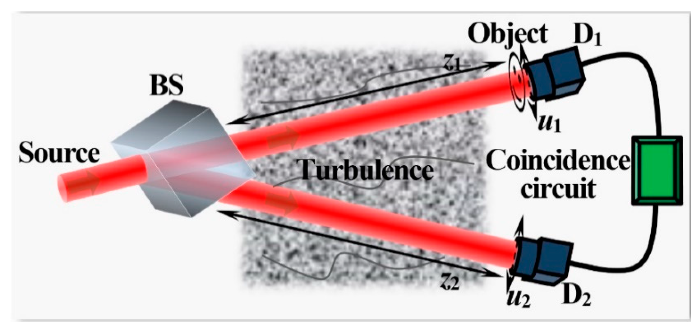
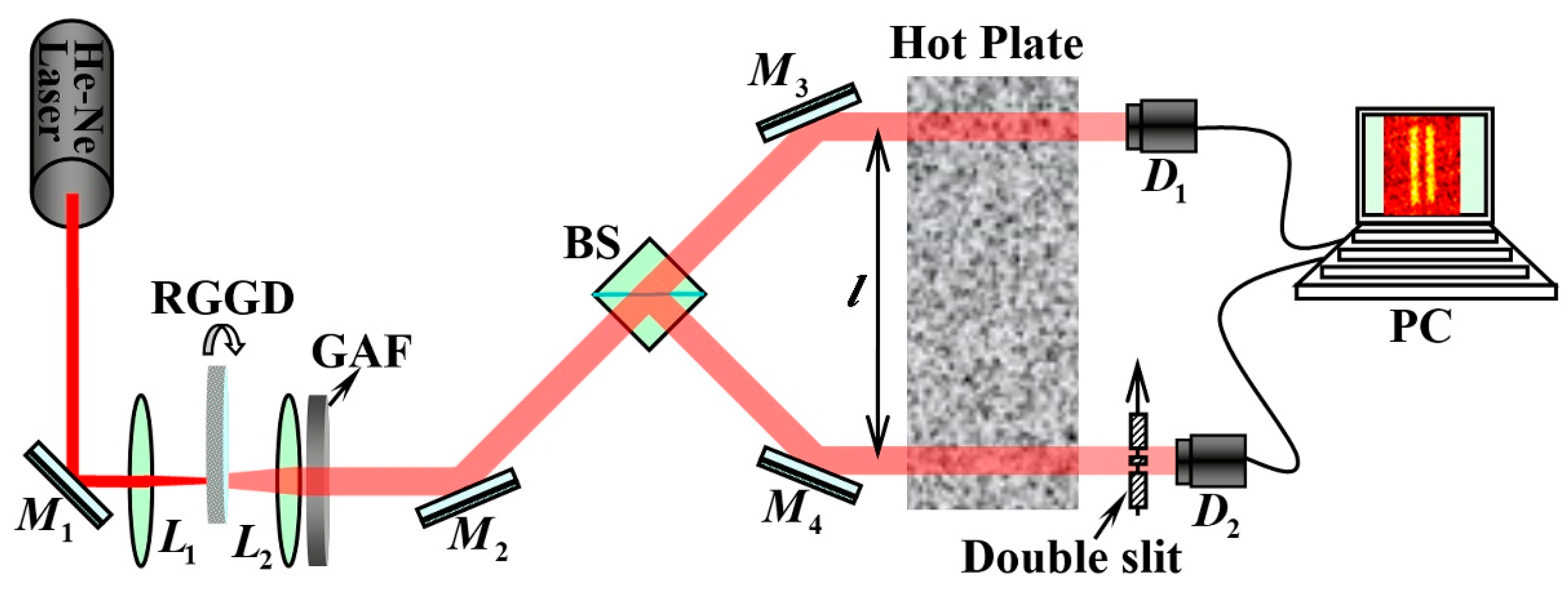
Figure 1 shows the typical GI optical system [20,21]. The light source is first split into two twin portions by the intensity beam splitter (BS), and then, two portions propagate through two distinct paths. One is a test path, which contains a bucket detector D₁ and an object. The object is close to D₁, and the distance from the source to D₁ is z₁. Another is a reference path, where a high spatial resolution single-photon detector D₂ is located at a distance z₂ from the source. Generally, both of two paths are in turbulence. The output signals from D₁ and D₂ are sent to a coincidence circuit to measure the forth-order correlation function (FOCF), i.e., intensity fluctuations. In order to observe the image information, the condition z₂ = z₁ = z should be satisfied. As shown in Figure 1, the turbulence is introduced in two optical paths.

Based on the optical coherence theory, the FOCF between the planes of $u_1$ and $u_2$ can be written as

$$\begin{array}{cc}\hfill G^{(2)}\left(u_1,u_2\right)& =\langle I\left(u_1\right)I\left(u_2\right)\rangle \hfill \\ & ={\displaystyle \underset{-\infty }{\overset{\infty }{\int }}{\displaystyle \underset{-\infty }{\overset{\infty }{\int }}{\displaystyle \underset{-\infty }{\overset{\infty }{\int }}{\displaystyle \underset{-\infty }{\overset{\infty }{\int }}{\langle E\left(x_1\right)E^{\ast }\left(x_2\right)E\left(x_3\right)E^{\ast }\left(x_4\right)\rangle }_s}}}}\hfill \\ & \times {\langle h_1\left(u_1,x_1\right)h_1^{\ast }\left(u_1,x_2\right)h_2\left(u_2,x_3\right)h_2^{\ast }\left(u_2,x_4\right)\rangle }_{m}d{x}_{1}d{x}_{2}d{x}_{3}d{x}_4,\hfill \end{array}$$

(1)

where $I\left(u\right)$ is the instantaneous intensity at point $u$ in the transverse plane of $u_i$ (i = 1, 2); ${\langle E\left(x_1\right)E^{\ast }\left(x_2\right)E\left(x_3\right)E^{\ast }\left(x_4\right)\rangle }_s$ is the FOCF of the light source, with $x$ being the coordinate in the source plane. The angle brackets with subscript “s” denote the ensemble average over the source fluctuations. “*” is the complex conjugate. 〈..m〉 stands for the ensemble average over the statistics of turbulence. $h_1$ and $h_2$ are the response functions of Path 1 and Path 2, respectively, given by:

$$h_1\left(u,x\right)={\left(\frac{i}{\lambda z_1}\right)}^{1/2}H\left(u\right)\exp \left[-\frac{i\pi }{\lambda z_1}{\left(u-x\right)}^2\right]\exp \left[{\psi }_1\left(u,x\right)\right],$$

(2)

$$h_2\left(u,x\right)={\left(\frac{i}{\lambda z_2}\right)}^{1/2}\exp \left[-\frac{i\pi }{\lambda z_2}{\left(u-x\right)}^2\right]\exp \left[{\psi }_2\left(u,x\right)\right],$$

(3)

$H\left(u\right)$ in Equation (2) represents the transmission function of the object. $\lambda$ is the wavelength; ${\psi }_1\left(u,x\right)$ and ${\psi }_2\left(u,x\right)$ are the complex phase perturbations introduced by the turbulence in Path 1 and Path 2, respectively. On substituting Equations (2) and (3) into Equation (1), after some rearrangement, it turns out to be:

$$\begin{array}{cc}\hfill G^{\left(2\right)}\left(u_1,u_2\right)& =\frac{1}{{\lambda }^2{z}_1{z}_2}{\displaystyle \underset{-\infty }{\overset{\infty }{\int }}{\displaystyle \underset{-\infty }{\overset{\infty }{\int }}{\displaystyle \underset{-\infty }{\overset{\infty }{\int }}{\displaystyle \underset{-\infty }{\overset{\infty }{\int }}d{x}_{1}d{x}_{2}d{x}_{3}d{x}_4{\left|H\left(u_1\right)\right|}^2{\langle E\left(x_1\right)E^{\ast }\left(x_2\right)E\left(x_3\right)E^{\ast }\left(x_4\right)\rangle }_s}}}}\hfill \\ & \hspace{1em}\times F_4\left(x_1,x_2,x_3,x_4;u_1,u_2\right)\exp \left[-\frac{ik}{2z_1}{\left(x_1-u_1\right)}^2\right]\exp \left[\frac{ik}{2z_1}{\left(x_2-u_1\right)}^2\right]\hfill \\ & \hspace{1em}\times \exp \left[-\frac{ik}{2z_2}{\left(x_3-u_2\right)}^2\right]\exp \left[\frac{ik}{2z_2}{\left(x_4-u_2\right)}^2\right],\hfill \end{array}$$

(4)

$F_4\left(x_1,x_2,x_3,x_4;u_2,u_2\right)$ in Equation (4) is the fourth-order coherence function of the turbulent medium, given by:

$$F_4\left(x_1,x_2,x_3,x_4;u_1,u_2\right)={\langle \exp \left[{\psi }_1\left(x_1,u_1\right)+{\psi }_1^{\ast }\left(x_2,u_1\right)+{\psi }_2\left(x_3,u_2\right)+{\psi }_2^{\ast }\left(x_4,u_2\right)\right]\rangle }_m,$$

(5)

Assume that the light source obeys Gaussian statistics with a zero mean. By applying the Gaussian moment theorem [41,42], the FOCF of the source can be expanded in terms of second-order correlation functions as follows:

$$\begin{array}{cc}\hfill {\langle E\left(x_1\right)E^{\ast }\left(x_2\right)E\left(x_3\right)E^{\ast }\left(x_4\right)\rangle }_s& ={\langle E\left(x_1\right)E^{\ast }\left(x_2\right)\rangle }_s{\langle E\left(x_3\right)E^{\ast }\left(x_4\right)\rangle }_s\hfill \\ & +{\langle E\left(x_1\right)E^{\ast }\left(x_4\right)\rangle }_s{\langle E^{\ast }\left(x_2\right)E\left(x_3\right)\rangle }_s,\hfill \end{array}$$

(6)

On substituting Equation (6) into Equation (4), we obtain the expression:

$$G^{\left(2\right)}\left(u_1,u_2\right)=I_4\left(u_1,u_2,z\right)+{\mathsf{\Gamma }}_4\left(u_1,u_2,z\right),$$

(7)

with:

$$\begin{array}{cc}\hfill I_4\left(u_1,u_2\right)& =\frac{1}{{\lambda }^2{z}_1{z}_2}{\displaystyle \underset{-\infty }{\overset{\infty }{\int }}{\displaystyle \underset{-\infty }{\overset{\infty }{\int }}{\displaystyle \underset{-\infty }{\overset{\infty }{\int }}{\displaystyle \underset{-\infty }{\overset{\infty }{\int }}d{x}_{1}d{x}_{2}d{x}_{3}d{x}_4{\left|H\left(u_1\right)\right|}^2{\langle E\left(x_1\right)E^{\ast }\left(x_2\right)\rangle }_s{\langle E\left(x_3\right)E^{\ast }\left(x_4\right)\rangle }_s}}}}\hfill \\ & \hspace{1em}\times F_4\left(x_1,x_2,x_3,x_4;u_1,u_2\right)\exp \left[-\frac{ik}{2z_1}{\left(x_1-u_1\right)}^2\right]\exp \left[\frac{ik}{2z_1}{\left(x_2-u_1\right)}^2\right]\hfill \\ & \hspace{1em}\times \exp \left[-\frac{ik}{2z_2}{\left(x_3-u_2\right)}^2\right]\exp \left[\frac{ik}{2z_2}{\left(x_4-u_2\right)}^2\right],\hfill \end{array}$$

(8)

$$\begin{array}{cc}\hfill {\mathsf{\Gamma }}_4\left(u_1,u_2\right)& =\frac{1}{{\lambda }^2{z}_1{z}_2}{\displaystyle \underset{-\infty }{\overset{\infty }{\int }}{\displaystyle \underset{-\infty }{\overset{\infty }{\int }}{\displaystyle \underset{-\infty }{\overset{\infty }{\int }}{\displaystyle \underset{-\infty }{\overset{\infty }{\int }}d{x}_{1}d{x}_{2}d{x}_{3}d{x}_4{\left|H\left(u_1\right)\right|}^2{\langle E\left(x_1\right)E^{\ast }\left(x_4\right)\rangle }_s{\langle E^{\ast }\left(x_2\right)E\left(x_3\right)\rangle }_s}}}}\hfill \\ & \hspace{1em}\times F_4\left(x_1,x_2,x_3,x_4;u_1,u_2\right)\exp \left[-\frac{ik}{2z_1}{\left(x_1-u_1\right)}^2\right]\exp \left[\frac{ik}{2z_1}{\left(x_2-u_1\right)}^2\right]\hfill \\ & \hspace{1em}\times \exp \left[-\frac{ik}{2z_2}{\left(x_3-u_2\right)}^2\right]\exp \left[\frac{ik}{2z_2}{\left(x_4-u_2\right)}^2\right].\hfill \end{array}$$

(9)

As we know from the GI scheme, the first term of Equation (7) represents the background noise, which does not contain any image information, while the second term contains the image information of the object. In atmospheric optics, it is usually assumed that the detector belongs to a “slow” detector. In this circumstance, three characteristic times satisfy the relation ${\tau }_s = {\tau }_u = {\tau }_a$, with ${\tau }_s$ being the characteristic time of the source fluctuations, ${\tau }_u$ being the response time (integrated time) of the detectors and ${\tau }_a$ being the characteristic time of the turbulence fluctuations. Thus, the detectors cannot perceive the instantaneous intensity fluctuations of the source due to ${\tau }_s = {\tau }_u$, but they can detect the intensity fluctuations induced by the turbulence. Under this condition, the second term on the right side of Equation (7) can be neglected, and the first term is proportional to the turbulence-induced scintillation index [43]. Thus, no image information can be obtained since the information of the image is contained in the second term. In order to acquire the ghost image, the detectors must act as the “fast detectors”, which satisfy the condition: ${\tau }_s = {\tau }_u = {\tau }_a$. Thus, the FOCF includes the first and second terms in Equation (7) simultaneously.

2.1. Bistatic Turbulence Case

In this situation, the complex phase perturbations in Path 1 and Path 2 are statistically independent. $F_4\left(x_1,x_2,x_3,x_4;u_2,u_2\right)$ can be simplified as:

$$F_4\left(x_1,x_2,x_3,x_4;u_1,u_2\right)={\langle \exp \left[{\psi }_1\left(x_1,u_1\right)+{\psi }_1^{\ast }\left(x_2,u_1\right)\right]\rangle }_m{\langle \exp \left[{\psi }_2\left(x_3,u_2\right)+{\psi }_2^{\ast }\left(x_4,u_2\right)\right]\rangle }_m.$$

(10)

By applying the Kolmogorov turbulence and quadratic approximation, Equation (10) takes the form [32]:

$$F_4\left(x_1,x_2,x_3,x_4;u_1,u_2\right)=\exp \left[-\frac{{\left(x_1-x_2\right)}^2}{{\rho }_{01}^2}\right]\exp \left[-\frac{{\left(x_3-x_4\right)}^2}{{\rho }_{02}^2}\right],$$

(11)

where ${\rho }_{01} = {\left(0.545C_{n1}^2{k}^2{z}_1\right)}^{-3/5}$ and ${\rho }_{02} = {\left(0.545C_{n2}^2{k}^2{z}_2\right)}^{-3/5}$ are the coherence lengths of a spherical wave in Path 1 and Path 2, respectively. $C_{n1}^2$ and $C_{n2}^2$ are the structure constants indicating the turbulence strength. k is the wave number of the source.

In order to evaluate Equation (7), we further assume that the light source is of a Gaussian–Schell model (GSM) beam, the mutual coherence function of which is expressed as [41,42]:

$$\langle E\left(x_i\right)E^{\ast }\left(x_j\right)\rangle =\exp \left[-\frac{x_i^2+x_j^2}{4{\sigma }_I^2}-\frac{{\left(x_i-x_j\right)}^2}{2{\sigma }_g^2}\right],$$

(12)

where ${\sigma }_I$ and ${\sigma }_g$ are the transverse beam width and transverse coherence width, respectively.

On substituting Equations (11) and (12) into Equations (8) and (9), with the help of a tensor method, we obtain the following expression:

$$\begin{array}{cc}\hfill I_4^{\left(b\right)}\left(u_1,u_2\right)& =\frac{1}{{\lambda }^2{\left[\det \left({\tilde{B}}^{-1}\right)\right]}^{1/2}}{\displaystyle \underset{-\infty }{\overset{\infty }{\int }}{\displaystyle \underset{-\infty }{\overset{\infty }{\int }}{\displaystyle \underset{-\infty }{\overset{\infty }{\int }}{\displaystyle \underset{-\infty }{\overset{\infty }{\int }}{\left|H\left(u_1\right)\right|}^2\exp \left(-\frac{ik}{2}{\tilde{\mathbf{r}}}^T{\tilde{M}}^{-1}\tilde{\mathbf{r}}\right)}}}}\exp \left(-\frac{ik}{2}{\tilde{\mathbf{r}}}^T\tilde{S}\tilde{\mathbf{r}}\right)\hfill \\ & \hspace{1em}\times \exp \left[-\frac{ik}{2}\left({\tilde{\mathbf{r}}}^T\tilde{B}\tilde{\mathbf{r}}-2{\tilde{\mathbf{r}}}^T\tilde{B}\tilde{\mathbf{u}}\right)\right]d\tilde{\mathbf{r}},\hfill \end{array}$$

(13)

$$\begin{array}{cc}\hfill {\mathsf{\Gamma }}_4^{\left(b\right)}\left(u_1,u_2\right)& =\frac{1}{{\lambda }^2{\left[\det \left({\tilde{B}}^{-1}\right)\right]}^{1/2}}{\displaystyle \underset{-\infty }{\overset{\infty }{\int }}{\displaystyle \underset{-\infty }{\overset{\infty }{\int }}{\displaystyle \underset{-\infty }{\overset{\infty }{\int }}{\displaystyle \underset{-\infty }{\overset{\infty }{\int }}{\left|H\left(u_1\right)\right|}^2\exp \left(-\frac{ik}{2}{\tilde{\mathbf{r}}}^T{\tilde{N}}^{-1}\tilde{\mathbf{r}}\right)\exp \left(-\frac{ik}{2}{\tilde{\mathbf{r}}}^T\tilde{S}\tilde{\mathbf{r}}\right)}}}}\hfill \\ & \hspace{1em}\times \exp \left(-\frac{ik}{2}{\tilde{\mathbf{r}}}^T\tilde{B}\tilde{\mathbf{r}}+ik{\tilde{\mathbf{r}}}^T\tilde{B}\tilde{\mathbf{u}}\right)d\tilde{\mathbf{r}},\hfill \end{array}$$

(14)

here, ${\tilde{\mathbf{r}}}^T = \left(x_1,x_2,x_3,x_4\right)$, ${\tilde{\mathbf{u}}}^T = \left(u_1,u_2,u_3,u_4\right)$ with the superscript being the transpose symbol and:

$${\tilde{M}}^{-1}=\left(\begin{array}{cc}{\overline{M}}_1^{-1}& 0I\\ 0I& {\overline{M}}_1^{-1}\end{array}\right),\tilde{S}=\left(\begin{array}{cc}{\overline{S}}_1& 0I\\ 0I& {\overline{S}}_2\end{array}\right),$$

(15)

$$\tilde{B}=\left(\begin{array}{cc}{\overline{B}}_1& 0I\\ 0I& {\overline{B}}_1\end{array}\right),{\tilde{N}}^{-1}=\left(\begin{array}{cc}{\overline{N}}_1^{-1}& {\overline{N}}_2^{-1}\\ {\overline{N}}_2^{-1}& {\overline{N}}_1^{-1}\end{array}\right),$$

(16)

where ${\tilde{M}}^{-1}$, $\tilde{S}$, $\tilde{B}$ and ${\tilde{N}}^{-1}$ are $4\times 4$ matrices; I is a $2\times 2$ unit matrix. ${\overline{M}}_1^{-1}$, ${\overline{S}}_1$, ${\overline{S}}_2$, ${\overline{N}}_1^{-1}$, ${\overline{N}}_2^{-1}$ and ${\overline{B}}_1$ are all $2\times 2$ matrices, given by:

$${\overline{M}}_1^{-1}=\left(\begin{array}{cc}-\frac{i}{k}\left(\frac{1}{2{\sigma }_I^2}+\frac{1}{{\sigma }_g^2}\right)& \frac{i}{k{\sigma }_g^2}\\ \frac{i}{k{\sigma }_g^2}& -\frac{i}{k}\left(\frac{1}{2{\sigma }_I^2}+\frac{1}{{\sigma }_g^2}\right)\end{array}\right),{\overline{N}}_1^{-1}=\left(\begin{array}{cc}-i\frac{\left[1/\left(2{\sigma }_I^2\right)+1/{\sigma }_g^2\right]}{k}& 0\\ 0& -i\frac{\left[1/\left(2{\sigma }_I^2\right)+1/{\sigma }_g^2\right]}{k}\end{array}\right),$$

(17)

$${\overline{N}}_2^{-1}=\left(\begin{array}{cc}0& i/\left(k{\sigma }_g^2\right)\\ i/\left(k{\sigma }_g^2\right)& 0\end{array}\right),{\overline{S}}_1=\frac{-2i}{k}\left(\begin{array}{cc}1/{\rho }_{01}^2& -1/{\rho }_{01}^2\\ -1/{\rho }_{01}^2& 1/{\rho }_{01}^2\end{array}\right),$$

(18)

$${\overline{S}}_2=\frac{-2i}{k}\left(\begin{array}{cc}1/{\rho }_{02}^2& -1/{\rho }_{02}^2\\ -1/{\rho }_{02}^2& 1/{\rho }_{02}^2\end{array}\right),{\overline{B}}_1=\left(\begin{array}{cc}1/z& 0\\ 0& 1/z\end{array}\right),$$

(19)

After vector integrating over $\tilde{r}$, Equations (20) and (21) become:

$$I_4^{\left(b\right)}\left(u_1,u_2\right)=\frac{{\left|H\left(u_1\right)\right|}^2}{{\left[\det \left({\tilde{B}}^{-1}{\tilde{M}}^{-1}+{\tilde{B}}^{-1}\tilde{S}+\tilde{I}\right)\right]}^{1/2}}\exp \left(\frac{ik}{2}{\tilde{u}}^T{\tilde{M}}_{o1}^{-1}\tilde{u}\right),$$

(20)

$${\mathsf{\Gamma }}_4^{\left(b\right)}\left(u_1,u_2\right)=\frac{{\left|H\left(u_1\right)\right|}^2}{{\left[\det \left({\tilde{B}}^{-1}{\tilde{M}}^{-1}+{\tilde{B}}^{-1}\tilde{S}+\tilde{I}\right)\right]}^{1/2}}\exp \left(\frac{ik}{2}{\tilde{u}}^T{\tilde{N}}_{o1}^{-1}\tilde{u}\right),$$

(21)

with $M_{o1}^{-1}=\tilde{B}{\left({\tilde{N}}^{-1}+\tilde{S}+\tilde{B}\right)}^{-1}\tilde{B}$. The superscript “(b)” denotes the case of bistatic turbulence. Equations (20) and (21) represent the background noise and the ghost image information terms, respectively.

2.2. Monostatic Turbulence Case

In this case, $F_4\left(x_1,x_2,x_3,x_4;u_2,u_2\right)$ cannot be separated as the product of the ensemble average over the second-order statistics of ${\psi }_1$ and that of ${\psi }_2$ due to that the turbulence in two paths being statistically correlated. There are some theoretical approximation models to describe this process [43,44,45,46,47]. Here, we adopt the theoretical model based on Wang’s analysis [43], and $F_4$ is expressed as:

$$\begin{array}{l}{F}_4\left(x_1,x_2,x_3,x_4,u_1,u_2\right)=\exp \left[-0.5D_{\psi }\left(x_1-x_2,0\right)-0.5D_{\psi }\left(x_1-x_4,u_1-u_2\right)-0.5D_{\psi }\left(x_2-x_3,u_1-u_2\right)\right]\\ \hspace{1em}\times \exp \left[-0.5D_{\psi }\left(x_3-x_4,0\right)+0.5D_{\psi }\left(x_2-x_4,u_1-u_2\right)+0.5D_{\psi }\left(x_1-x_3,u_1-u_2\right)\right]\\ \hspace{1em}\times \exp \left[2B_x\left(x_2-x_4,u_1-u_2\right)+2B_x\left(x_1-x_3,u_1-u_2\right)\right]\\ \hspace{1em}\times \exp \left[i{D}_{xs}\left(x_2-x_4,u_1-u_2\right)-i{D}_{xs}\left(x_1-x_3,u_1-u_2\right)\right],\end{array}$$

(22)

where $D_{\psi }\left(x_i,x_j,u_d\right)$ is the wave structure function:

$$D_{\psi }\left(x_i,x_j,u_d\right)=\left[{\left(x_i-x_j\right)}^2+\left(x_i-x_j\right)u_d+u_d^2\right]/{\rho }_0^2, \left(i,j=1,2,3,4\right),$$

(23)

Here, ${\rho }_0 = {\left(0.546C_n^2{k}^{2}z\right)}^{-3/5}$ is the coherence length of a spherical wave propagating in the turbulent medium, $u_d = u_1 – u_2$, and $C_n^2$ is the structure constant. $B_x = {\left(x\right)}_i – x_j,u_d$ is the log-amplitude correlation function, via:

$$B_x\left(x_i-x_j,u_d.\right)={\sigma }_{xs}^2-\frac{1}{2}\left(\frac{1}{{\rho }_0^2}-\frac{1}{{\rho }_x^2}\right)\left[{\left(x_i-x_j\right)}^2+u_d\left(x_i-x_j\right)+u_d^2\right]$$

(24)

where ${\sigma }_{xs}^2 = 0.124k^{7/6}{C}_n^2{z}^{11/6}$ is the variance of the log amplitude for a spherical wave, and ${\rho }_x = {\left(0.425C_n^2{k}^{13/6}{z}^{5/6}\right)}^{-1/2}$. $D_{xs}\left(x_i – x_j,u_d\right)$ is the log-amplitude phase structure function via:

$$D_{xs}\left(x_i-x_j,u_d\right)=\left[{\left(x_i-x_j\right)}^2+\left(x_i-x_j\right)u_d+u_d^2\right]/{\rho }_{xs}^2$$

(25)

where ${\rho }_{xs} = {\left(0.114C_n^2{k}^{13/6}{z}^{5/6}\right)}^{-1/2}$ is the coherence length of the log-amplitude and phase.

In the derivation of Equation (22), the Kolmogorov spectrum with zero inner scale and the quadratic approximation are used. The validation condition is ${\sigma }_{xs}^2 = 1$ for guaranteeing weak turbulence. On substituting Equations (12) and (22) into Equations (8) and (9), after some rearrangements, we rewrite Equations (8) and (9) in the following alternative tensor forms:

$$\begin{array}{l}{I}_4^{\left(m\right)}\left(u_1,u_2\right)=\frac{\exp \left(4{\sigma }_{xs}^2\right)}{{\lambda }^2{\left[\det \left({\tilde{B}}^{-1}\right)\right]}^{1/2}}{\displaystyle \underset{-\infty }{\overset{\infty }{\int }}{\displaystyle \underset{-\infty }{\overset{\infty }{\int }}{\displaystyle \underset{-\infty }{\overset{\infty }{\int }}{\displaystyle \underset{-\infty }{\overset{\infty }{\int }}{\left|H\left(u_1\right)\right|}^2\exp \left[-\frac{ik}{2}{\tilde{\mathbf{r}}}^T\left({\tilde{M}}^{-1}+\tilde{O}+\tilde{B}\right)\tilde{\mathbf{r}}\right]}}}}\\ \hspace{1em}\times \exp \left[ik{\tilde{\mathbf{r}}}^T\left(\tilde{P}+\tilde{B}\right)\tilde{\mathbf{u}}\right]\exp \left(-\frac{ik}{2}{\tilde{\mathbf{u}}}^T\tilde{Q}\tilde{\mathbf{u}}\right)d\tilde{\mathbf{r}},\end{array}$$

(26)

$$\begin{array}{l}{\mathsf{\Gamma }}_4^{\left(m\right)}\left(u_1,u_2\right)=\frac{\exp \left(4{\sigma }_{xs}^2\right)}{{\lambda }^2{\left[\det \left({\tilde{B}}^{-1}\right)\right]}^{1/2}}{\displaystyle \underset{-\infty }{\overset{\infty }{\int }}{\displaystyle \underset{-\infty }{\overset{\infty }{\int }}{\displaystyle \underset{-\infty }{\overset{\infty }{\int }}{\displaystyle \underset{-\infty }{\overset{\infty }{\int }}{\left|H\left(u_1\right)\right|}^2\exp \left(-\frac{ik}{2}{\tilde{\mathbf{r}}}^T{\tilde{N}}^{-1}\tilde{\mathbf{r}}\right)\exp \left(-\frac{ik}{2}{\tilde{\mathbf{r}}}^T\tilde{O}\tilde{\mathbf{r}}\right)}}}}\\ \hspace{1em}\times \exp \left(ik{\tilde{\mathbf{r}}}^T\tilde{P}\tilde{\mathbf{u}}\right)\exp \left(-\frac{ik}{2}{\tilde{\mathbf{u}}}^T\tilde{Q}\tilde{\mathbf{u}}\right)\exp \left(-\frac{ik}{2}{\tilde{\mathbf{r}}}^T\tilde{B}\tilde{\mathbf{r}}+ik{\tilde{\mathbf{r}}}^T\tilde{B}\tilde{\mathbf{u}}\right)d\tilde{\mathbf{r}}.\end{array}$$

(27)

Here, $\tilde{O} = \left(\begin{array}{cc}{\overline{\begin{array}{c}\\ O\end{array}}}_1& {\overline{O}}_2\\ {\overline{O}}_3& {\overline{O}}_4\end{array}\right)$, $\tilde{P} = \left(\begin{array}{cc}{\overline{P}}_1& -{\overline{P}}_1\\ -{\overline{P}}_1& {\overline{P}}_1\end{array}\right)$, $\tilde{Q} = \left(\begin{array}{cc}{\overline{Q}}_1& -{\overline{Q}}_1\\ -{\overline{Q}}_1& {\overline{Q}}_1\end{array}\right)$ are $4 \times 4$ matrices, with ${\overline{O}}_1 = \frac{2i}{k}\left(\begin{array}{cc}a& -1/{\rho }_0^2\\ -1/{\rho }_0^2& a^{\ast }\end{array}\right)$, ${\overline{O}}_2 = \frac{2i}{k}\left(\begin{array}{cc}1/{\rho }_x^2-i/{\rho }_{xs}^2& -1/{\rho }_0^2\\ -1/{\rho }_0^2& 1/{\rho }_x^2+i/{\rho }_{xs}^2\end{array}\right)$, ${\overline{P}}_1 = -\frac{i}{k}\left(\begin{array}{cc}b& 0\\ 0& b^{\ast }\end{array}\right)$, and ${\overline{Q}}_1 = -\frac{2i}{k}\left(1/{\rho }_0^2-1/{\rho }_x^2\right)I$ being $2 \times 2$ matrices and $a = 2/{\rho }_{0 }^2-1/{\rho }_x^2+i/{\rho }_{xs}^2$, $b = -1/{\rho }_{0 }^2+1/{\rho }_x^2-i/{\rho }_{xs}^2$.

After vector integrating over $\tilde{r}$, we obtain the expressions:

$$I_4^{\left(m\right)}\left(u_1,u_2\right)=\frac{\exp \left(4{\sigma }_{xs}^2\right){\left|H\left(u_1\right)\right|}^2}{{\left[\det \left({\tilde{B}}^{-1}{\tilde{M}}^{-1}+{\tilde{B}}^{-1}\tilde{O}+\tilde{I}\right)\right]}^{1/2}}\exp \left[\frac{ik}{2}{\tilde{\mathbf{u}}}^T\left({\tilde{M}}_o-\tilde{Q}\right)\tilde{\mathbf{u}}\right],$$

(28)

$${\mathsf{\Gamma }}_4^{\left(m\right)}\left(u_1,u_2\right)=\frac{\exp \left(4{\sigma }_{xs}^2\right){\left|H\left(u_1\right)\right|}^2}{{\left[\det \left({\tilde{B}}^{-1}{\tilde{N}}^{-1}+{\tilde{B}}^{-1}\tilde{O}+\tilde{I}\right)\right]}^{1/2}}\exp \left[\frac{ik}{2}{\tilde{\mathbf{u}}}^T\left({\tilde{N}}_o-\tilde{Q}\right)\tilde{\mathbf{u}}\right],$$

(29)

with ${\tilde{M}}_0 = \left(\tilde{P} + \tilde{B}\right){\left({\tilde{M}}^{-1} +\widetilde{ O} + \tilde{B}\right)}^{-1}\left(\tilde{P} + \tilde{B}\right)$, ${\tilde{N}}_0 = \left(\tilde{P} + \tilde{B}\right){\left({\tilde{N}}^{-1} +\widetilde{ O} + \tilde{B}\right)}^{-1}\left(\tilde{P} + \tilde{B}\right)$, and $\tilde{I}$ is a $4 \times 4$ unit matrix. The superscript “(m)” denotes the monostatic turbulence case. Equations (28) and (29) are the main results in this paper for analyzing the quality and visibility of the ghost image in monostatic turbulence.

3. Numerical Examples and Analysis

In this section, we investigate the visibility and quality of the ghost image both in bistatic and monostatic turbulences through numerical examples. The wavelength of light in the calculation is set as $\mathsf{\lambda } = 632.8 \mathrm{nm}$, and the constant structures $C_n^2 = C_{n1}^2 = C_{n2}^2$ were fixed in the following numerical examples. The object is a double slit with slit width $a = 0.6 \mathrm{mm}$, and the distance of two slits $d = 1.2 \mathrm{mm}$; the beam width and the coherence width of the sources are ${\sigma }_I = 4 \mathrm{mm}$ and ${\sigma }_g = 0.3 \mathrm{mm}$, respectively. Because the detector D₁ is a bucket detector, then after integrating over u₁, the two normalized correlation functions are defined as:

$$g^{\left(k\right)}\left(u_2,z\right)=\frac{{\displaystyle {\int }_{-\infty }^{\infty }{G}^{\left(2\right)\left(k\right)}\left(u_1,u_2,z\right)d{u}_1}}{{\displaystyle {\int }_{-\infty }^{\infty }{I}_4^{\left(k\right)}\left(u_1,u_2,z\right)d{u}_1}},\left(k=m,b\right),$$

(30)

$${\gamma }^{\left(k\right)}\left(u_2,z\right)=\frac{{\displaystyle {\int }_{-\infty }^{\infty }{\mathsf{\Gamma }}_4^{\left(k\right)}\left(u_1,u_2,z\right)d{u}_1}}{{\left[{\displaystyle {\int }_{-\infty }^{\infty }{\mathsf{\Gamma }}_4^{\left(k\right)}\left(u_1,u_2,z\right)d{u}_1}\right]}_{\max }},\left(k=m,b\right),$$

(31)

the superscripts k = m and k = b denote the case of monostatic and bistatic turbulences, respectively. The subscript “max” in Equation (31) denotes the maximum value of ${\mathsf{\Gamma }}_4$. $g^{\left(k\right)}\left(u_2,z\right)$ in Equation (30) stands for the FOCF normalized by the background noise, and ${\gamma }^{\left(k\right)}\left(u_2,z\right)$ denotes the normalized image information subtracting out the background noise. The visibility of ghost image is defined as [17]:

$$V^{\left(k\right)}=\frac{{\left[g^{\left(k\right)}\left(u_2,z\right)\right]}_{\max }-{\left[g^{\left(k\right)}\left(u_2,z\right)\right]}_{\min }}{{\left[g^{\left(k\right)}\left(u_2,z\right)\right]}_{\max }+{\left[g^{\left(k\right)}\left(u_2,z\right)\right]}_{\min }},$$

(32)

where “min” in Equation (32) denotes the minimum value of $g^{\left(k\right)}\left(u_2,z\right)$.

The distance from the source to detector D₁ or D₂ in the calculation is 3 m, and the constant structure $C_n^2$ is relatively large within the range ${10}^{-10} {\mathrm{m}}^{-2/3} – {10}^{-12} {\mathrm{m}}^{-2/3}$, which is the typical parameter in the laboratory.

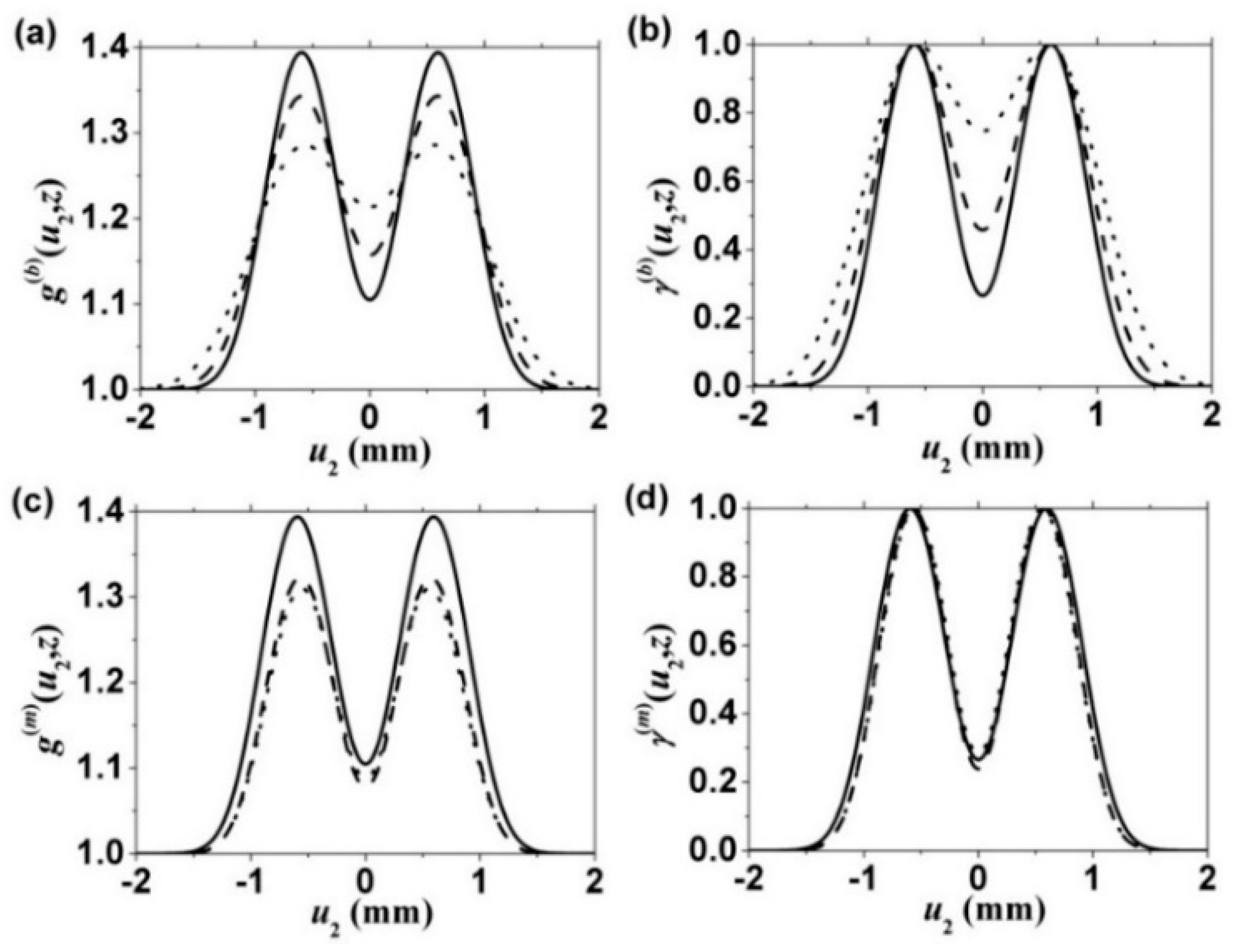
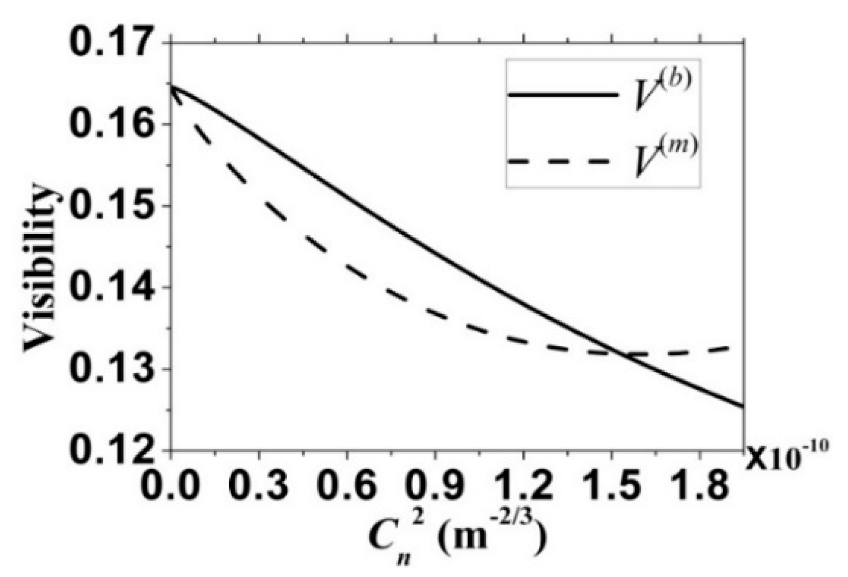
Figure 2 illustrates the values of $g^{\left(k\right)}\left(u_2,z\right)$ and ${\gamma }^{\left(k\right)}\left(u_2,z\right)$ against u₂ for different values of $C_n^2$. For the convenience of comparison, the ghost image in free space ($C_n^2 = 0$) is also plotted in Figure 2 (solid lines). For the case of bistatic turbulence, one sees from Figure 2a,b that the quality of the image degrades as the turbulence strength increases. This result is consistent with that discussed in [32]. In monostatic turbulence, the quality of the image keeps unchanged with the increase of turbulence compared to that in free space (see in Figure 2d), if we subtract out the background noise. It seems that the image is immune to the turbulence, which agrees well with the experiment results in [39]. To display the visibility of the image of the double slit in two types of turbulence, we plot in Figure 3 the visibility of the image as a function of the constant structure $C_n^2$. One can see that the visibility drops as the strength of the turbulence increases both in monostatic and bistatic cases. It decreases much faster in the monostatic case than that in bistatic case when $C_n^2 < 1.5 \times {10}^{-10} {\mathrm{m}}^{-2/3}$, while with the further increase of $C_n^2$, the situation is inversed.

Why are the visibility and quality of the image different in monostatic and bistatic turbulences? There are two main factors in atmospheric turbulence affecting the measured FOCF in the GI system due to the random fluctuation of the refraction index in the atmosphere. One is the beam wander, i.e., the random displacement of the beam position in the receiver plane. Another is the scintillation, which means random intensity fluctuation occurs. It is known that the ghost image arises from the intensity fluctuations of the light beams from test and reference paths in the GI system. For the case of monostatic turbulence, the beam wander and scintillation induced by the turbulence in two optical paths are exactly the same. In a sense, the intensity correlation from two paths is not destroyed by the turbulence. The quality of the image can keep unchanged in the monostatic turbulence. When the turbulence is bistatic, the beam wanders in two optical paths behave differently. At a certain moment, the position of the beam spot in one path drifts upwards, while in another path, it drifts downwards. The turbulence-induced scintillations in two paths are also not synchronous. Such turbulence acts as a disturber destroying the original intensity correlation between two paths. As a consequence, the quality of the image degrades. The visibility of the image is closely related to the coherence width of the beam. The smaller the coherence width is, the lower the visibility of the image is [13]. It is known that the turbulence deteriorates the transverse coherence width of the beam on propagation, while beam propagation will increase the coherence width due to diffraction. However, in the laboratory, the propagation distance is relatively short. The turbulence plays a dominant role in affecting the beam coherence width. Therefore, the visibility of the ghost image decreases with the increase of the strength of the turbulence.

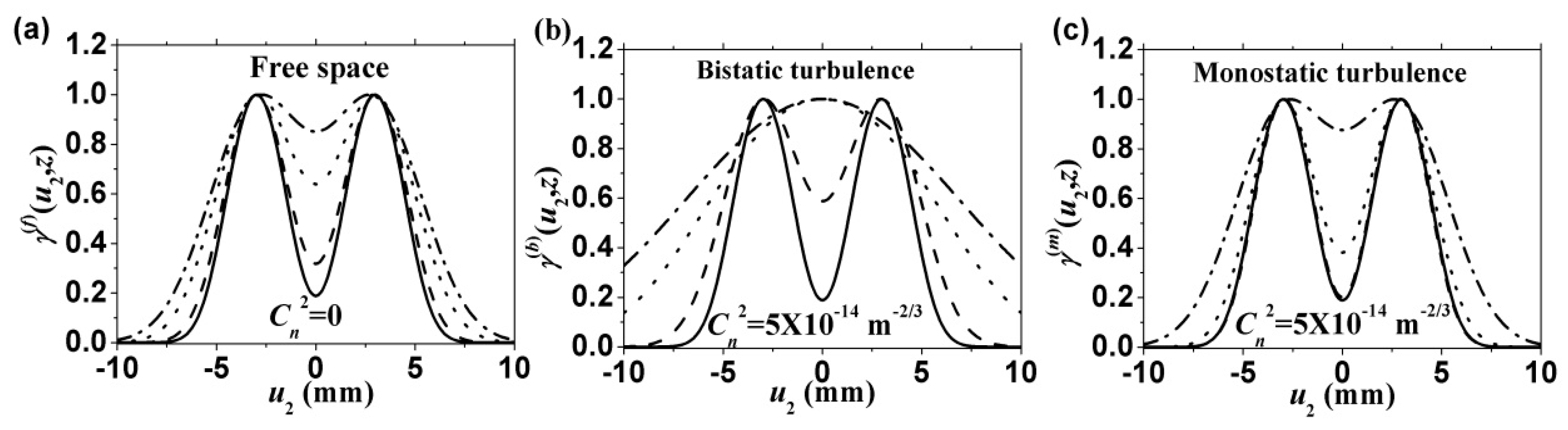
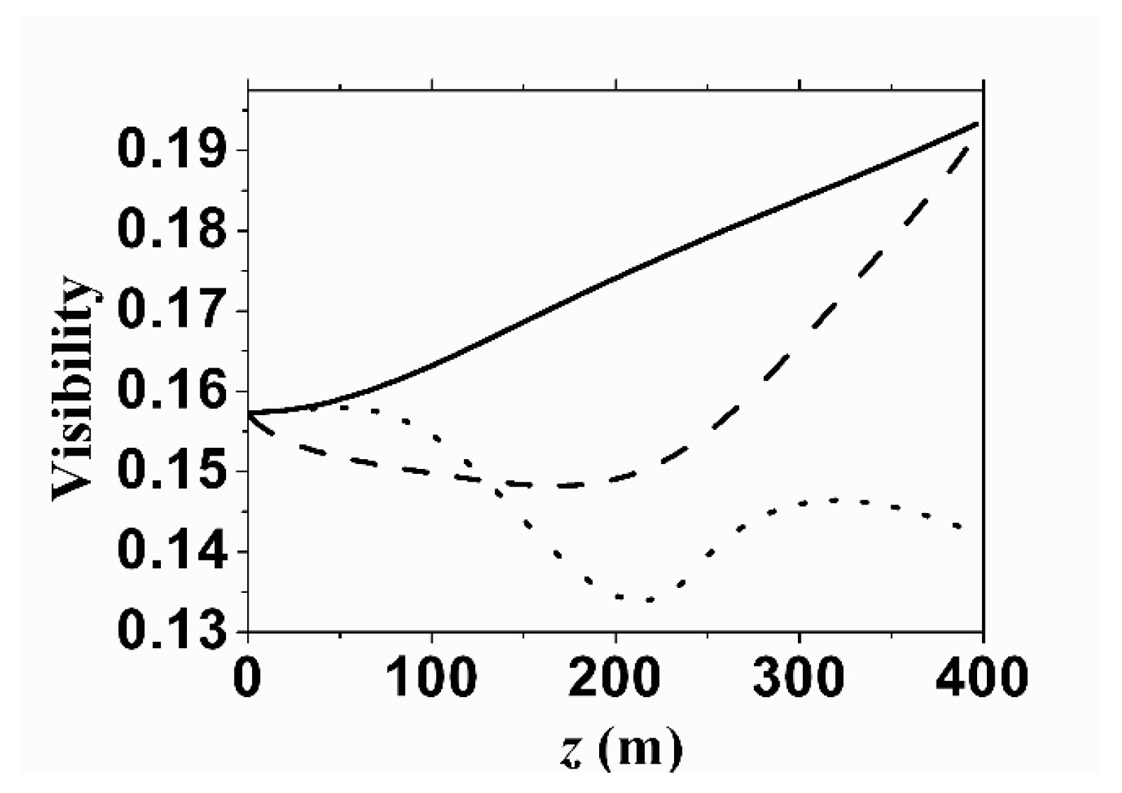
Let us now turn to study the characteristics of the GI when the distance from the light source to the object is an order of a hundred meters. Different from the short distance range, the propagation effect of the light may have significant effects on the visibility and quality of the image. In free space, the transverse coherence width ${\sigma }_g\left(z\right)$ of the light will become large on propagation. Thus, the quality of image will be worse, and the visibility of image increases due to the increase of ${\sigma }_g\left(z\right)$ [13]. While in the presence of turbulence, it will prevent the increase of ${\sigma }_g\left(z\right)$ on propagation [48]. As a consequence, the ghost image can remain for a long propagation distance, compared to that in free space. Figure 4 shows the image of the double slit at several propagation distances, e.g., z = 1 m, 150 m, 300 m and 400 m through monostatic and bistatic turbulences. For comparison, the image in free space is plotted in Figure 4a. The parameters used are chosen to be ${\sigma }_I = 15 \mathrm{mm}$, ${\sigma }_g = 1.5 \mathrm{mm}$, $C_n^2 = 5 \times {10}^{-14} {\mathrm{m}}^{-2/3}$, $a = 3 \mathrm{mm}$ and $d = 6 \mathrm{mm}$. In free space, the image of the double slit is blurred gradually as the propagation distance increases, as expected. This is caused by the increase of the transverse coherence width of the light on free-space propagation. In bistatic turbulence, the image degrades much faster than that in free space as the propagation distance increases due to the statistical independence of the turbulence in two paths. In monostatic turbulence, the quality of the image is better than that in free space in the propagation range from 0–400 m. Such turbulence displays the positive effects on the formation of the image. Figure 5 shows the dependence of the visibility of the ghost image on the propagation distance in free space, monostatic and bistatic turbulence. The parameters used in Figure 5 are the same as those in Figure 4. The visibility increases as the propagation distance increases since the coherence width of the beam increases due to beam diffraction. In the presence of turbulence, it will deteriorate the coherence width. The effect of the diffraction and turbulence on the transverse coherence width is different, making the variation of the visibility with propagation distance hard to predict.

4. Experimental Measurement of the Ghost Image through Monostatic and Bistatic Turbulence in the Lab

In this section, we carry out the lensless GI experiment through thermally-induced turbulence in the laboratory. The schematic for the experiment setup is shown in Figure 6.

A He-Ne laser beam operated at $\mathsf{\lambda } = 632.8 \mathrm{nm}$ is reflected by the mirror M₁, then focused onto a rotating ground glass disk (RGGD) by the lens L₁, then passes through the collimation lens L₂ and the Gaussian amplitude filter (GAF), which are used to collimate the light from RGGD and shape the intensity distribution of the light into the Gaussian profile, respectively. The beam emerging from the GAF can be regarded as the GSM source, the second-order correlations of the electric fields of which are described by Equation (12). The beam width and the coherence width are determined by the transmission radius of the GAF and the beam spot size on the RGGD, respectively. Note that the GSM source is not the unique source for realizing ghost imaging. Light sources with low spatial coherence such as sunlight and halogen lamps can serve as the illuminations in ghost imaging systems [49,50]. Perhaps, the light generated by a superluminescent diode is also a good candidate [51]. The generated source is split into two paths by the intensity beam splitter (BS). The transmitted beam is received by the detector D₁ after being reflected by the mirror M₃, and the reflected beam is received by the detector D₂. An object is placed against D₂. The output signals from D₁ and D₂ are sent to a computer to measure the FOCF. A $35 \mathrm{cm} \times 50 \mathrm{cm}$ hot plate is located in two paths to produce the thermally-induced turbulence. The strength of the turbulence is controlled by the temperature of the hot plate T. As seen in Figure 6, the distance between two paths after M₃ and M₄ is l. In our experiment, we modulate the distance l to control the monostatic or bistatic turbulence. If l = 0, the two optical paths from source to D₁ and from source to D₂ experience the same turbulence exactly. Therefore, the statistics of the turbulence is correlated, belonging to monostatic turbulence. When l is large enough, the correlation of the turbulence between two paths degrades, which means the statistics of turbulence in two paths are independent, degenerating to bistatic turbulence.

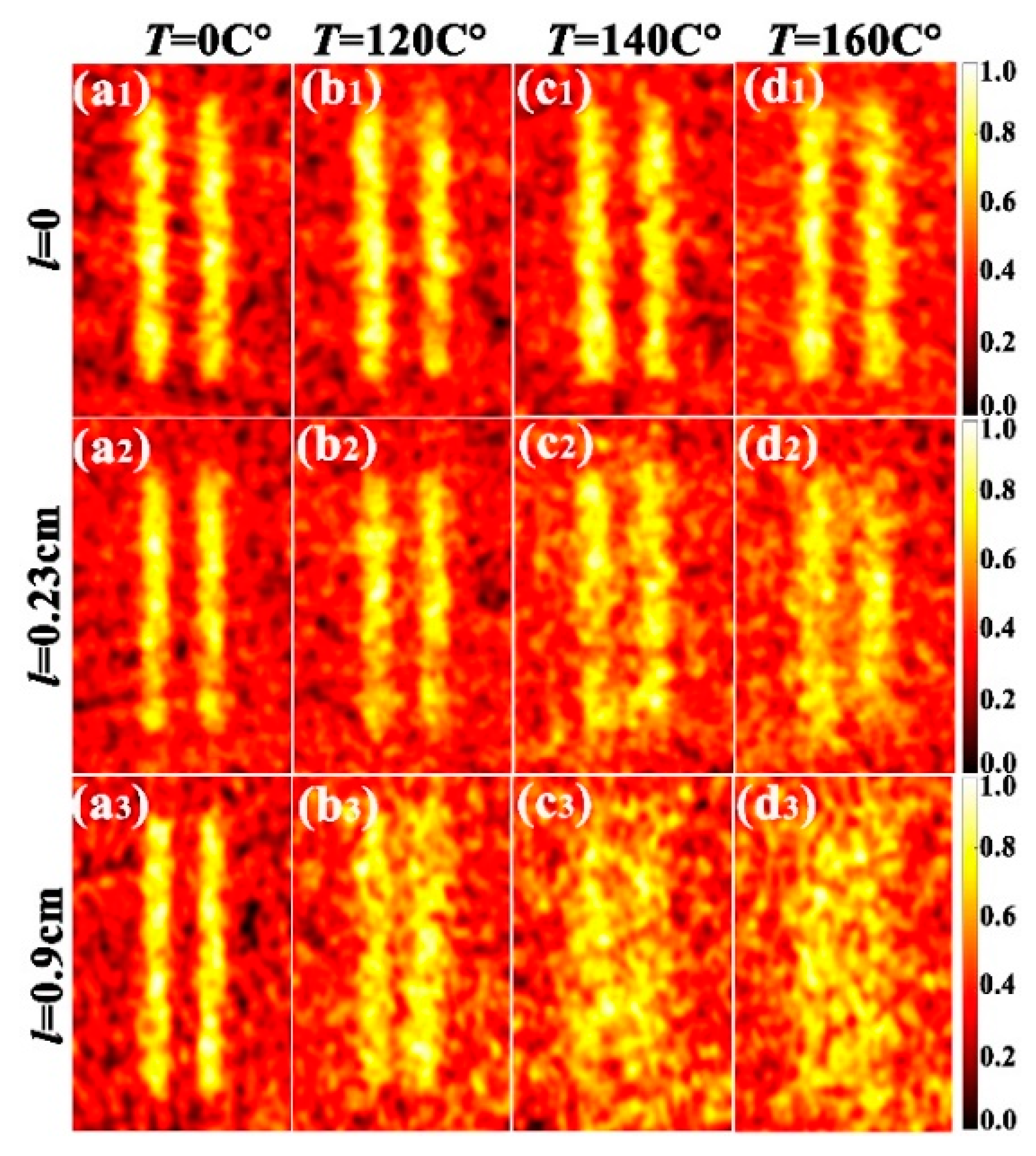
In the experiment, the object we used is a double slit with slit width $a = 0.6 \mathrm{mm}$ and the distance of two slits $d = 1.2 \mathrm{mm}$, corresponding to the numerical simulation in Figure 2. The beam width and the coherence width of the source measured from the experiment are ${\mathsf{\sigma }}_I = 4.0 \mathrm{mm}$ and ${\mathsf{\sigma }}_g = 0.3 \mathrm{mm}$, respectively. The distance from the source plane to D₁ or D₂ is about 1.0 m. In our experiment, D₁ and D₂ recorded 3000 frames with the frames per second (FPS) being 30, respectively, and then, the data were used to reconstruct the ghost image using the MATLAB software. The total time for obtaining one ghost image was about 140 s. Figure 7 presents the experiment results of the ghost image of the double slit with several different l and temperature T. the measured quantity of the image in the experiment is:

$$g_n^{(k)}=\frac{g^{\left(k\right)}\left(u_2,z\right)-1}{{[g^{\left(k\right)}\left(u_2,z\right)]}_{\max }},\left(k=m,b\right).$$

(33)

We see from Figure 7a₁–d₁ that the turbulence almost has no effect on the quality of the image in the monostatic case when the temperature of the hot plate is from 0–160 °C. As the distance l increases, the image is gradually blurred by the turbulence-induced degradation as the strength of the turbulence increases (see Figure 7a₂–d₂). When $l = 0.9 \mathrm{cm}$, the turbulence in two paths develop into the bistatic case, and no image information can be obtained for the temperatures $T = 160$ °C and (see Figure 7a₃–d₃). The distance l is closely related to the types of the turbulence. Our experimental results are consistent with the theoretical analysis in Section 2.

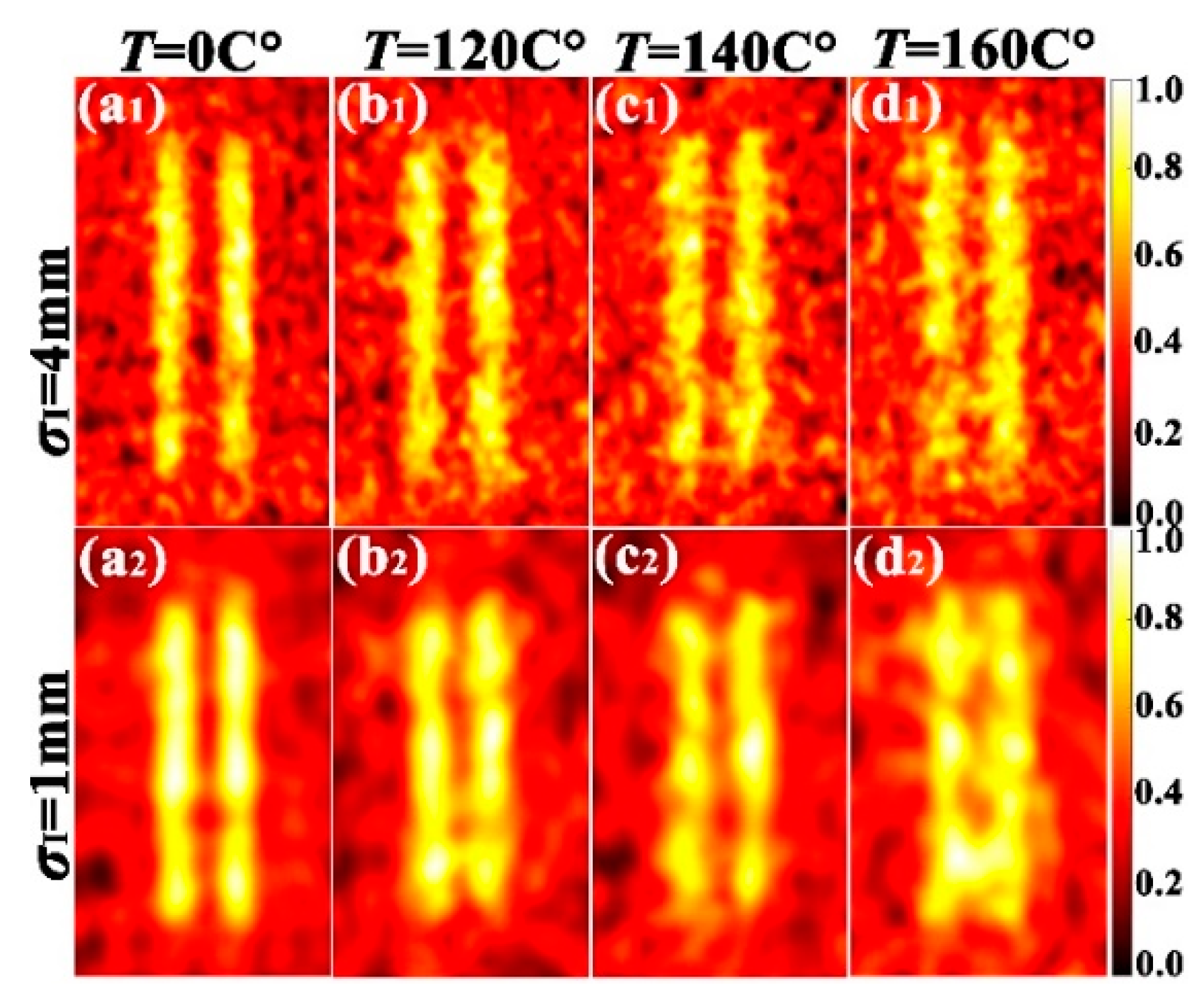
Next, we investigate the effects of the initial beam width on the quality of the image through the turbulence. Figure 8 shows the ghost image of the double slit at propagation distance $z = 0.5 \mathrm{m}$ for different hot plates’ temperatures with the initial beam width being ${\mathsf{\sigma }}_I = 4 \mathrm{mm}$ (first row) and ${\mathsf{\sigma }}_I = 1 \mathrm{mm}$ (second row). The coherence width of the source is the same as that in Figure 6. One sees that the image quality has not much difference under the same strength of turbulence, while the image seems smoother in the second row than that in the first row. As we know, the beam size and coherence width increase on propagation due to diffraction. The smaller the initial beam width is, the faster the increase of the transverse coherence width on propagation is. Thus, the coherence width for ${\mathsf{\sigma }}_I = 1 \mathrm{mm}$ is larger than that for ${\mathsf{\sigma }}_I = 4 \mathrm{mm}$ in the receiver plane, implying that the speckle size in a single realization of the intensity profile for ${\mathsf{\sigma }}_I = 1 \mathrm{mm}$ is relatively larger, which leads to a smoother image.

Because our experiment was carried out indoors with the help of the optical table and the hot plane, whose sizes are limited, we were not able to show more experimental results about the influence of the propagation distance z on the quality and visibility of the ghost image although the propagation distances in Figure 7 and Figure 8 are different. We plan to study the influence of the propagation distance on the ghost image in outdoor real turbulence in the future.

5. Conclusions

As a summary, we have studied the quality and visibility of the GI through monostatic and bistatic turbulences, both theoretically and experimentally. Analytical expressions for the FOCFs, which contain the background noise and the image information, are derived for the cases of monostatic and bistatic turbulences with the help of a tensor method. It was found that the visibility and the quality of the image in two types of atmospheric turbulences were different. In bistatic turbulence, the visibility and the quality of the image all degraded by the turbulence due to the statistical independence of the two paths in the GI system. In monostatic turbulence, the quality of the image can keep invariant as that in free space in some range of turbulence strength, whereas the visibility decreases with the increase of the turbulence. When the distance from the light source to the detection plane is an order of a hundred meters, the GI information can remain a longer distance in monostatic turbulence than that in the bistatic case under the same condition. The experiments for GI through monostatic and bistatic turbulences were demonstrated in the laboratory. Our results agree well with the theoretical predictions and are consistent with the experiment results in [39].

References

- Strekalov, D.V.; Sergienko, A.V.; Klyshko, D.N.; Shih, Y.H. Observation of Two-photon “Ghost” interference and diffraction. Phys. Rev. Lett. 1995, 74, 3600–3603. [Google Scholar] [CrossRef] [PubMed]
- Pittman, T.B.; Shih, Y.H.; Strekalov, D.V.; Sergienko, A.V. Optical imaging by means of two-photon quantum entanglement. Phys. Rev. A 1995, 52, R3429–R3432. [Google Scholar] [CrossRef] [PubMed]
- Bennink, R.S.; Bentley, S.J.; Boyd, R.W. “Two-photon” coincidence imaging with a classical source. Phys. Rev. Lett. 2002, 89, 113601. [Google Scholar] [CrossRef] [PubMed]
- Gatti, A.; Brambilla, E.; Bache, M.; Lugiato, L.A. Ghost imaging with thermal light: Comparing entanglement and classical correlation. Phys. Rev. Lett. 2004, 93, 093602. [Google Scholar] [CrossRef] [PubMed]
- Valencia, A.; Scarcelli, G.; D’Angelo, M.; Shih, Y. Two-photon imaging with thermal light. Phys. Rev. Lett. 2005, 94, 063601. [Google Scholar] [CrossRef] [PubMed]
- Gatti, A.; Bache, M.; Magatti, D.; Brambilla, E.; Ferri, F.; Lugiato, L.A. Coherent imaging with pseudothermal incoherent light. J. Mod. Opt. 2006, 53, 739–760. [Google Scholar] [CrossRef]
- Zhang, D.; Zhai, Y.; Wu, L.; Chen, X. Correlated two-photon imaging with true thermal light. Opt. Lett. 2005, 30, 2354–2356. [Google Scholar] [CrossRef] [PubMed]
- Cheng, J.; Han, S. Incoherent coincidence imaging and its applicability in X-ray diffraction. Phys. Rev. Lett. 2004, 92, 093903. [Google Scholar] [CrossRef] [PubMed]
- Cao, D.; Xiong, J.; Wang, K. Geometrical optics in correlated imaging systems. Phys. Rev. A 2005, 71, 013801. [Google Scholar] [CrossRef]
- Chan, K.W.C.; O’Sullivan, M.N.; Boyd, R.W. High-order thermal ghost imaging. Opt. Lett. 2009, 34, 3343–3345. [Google Scholar] [CrossRef] [PubMed]
- Erkmen, B.I.; Shapiro, H. ghost imaging: From quantum to classical to computational. Adv. Opt. Photonics 2010, 2, 405–450. [Google Scholar] [CrossRef]
- Ferri, F.; Magatti, D.; Sala, V.G.; Gatti, A. Longitudinal coherence in thermal ghost imaging. Appl. Phys. Lett. 2008, 92, 261109. [Google Scholar] [CrossRef] [Green Version]
- Cai, Y.; Zhu, S. Ghost imaging with incoherent and partially coherent light radiation. Phys. Rev. E. 2005, 71, 056607. [Google Scholar] [CrossRef] [PubMed]
- Vidal, I.; Caetano, D.P.; Fonseca, E.J.S.; Hickmann, J.M. Effects of pseudothermal light source’s transverse size and coherence width in ghost-interference experiments. Opt. Lett. 2009, 34, 1450–1452. [Google Scholar] [CrossRef] [PubMed]
- Liu, H.; Han, S. Spatial longitudinal coherence length of a thermal source and its influence on lensless ghost imaging. Opt. Lett. 2008, 33, 824–826. [Google Scholar] [CrossRef] [PubMed]
- Bai, Y.; Liu, H.; Han, S. Transmission area and correlated imaging. Opt. Express 2007, 15, 6062–6068. [Google Scholar] [CrossRef] [PubMed]
- Cao, D.; Xiong, J.; Zhang, S.; Lin, L.; Gao, L.; Wang, K. Enhancing visibility and resolution in Nth-order intensity correlation of thermal light. Appl. Phys. Lett. 2008, 92, 201102. [Google Scholar] [CrossRef]
- Bai, Y.; Han, S. Ghost imaging with thermal light by third-order correlation. Phys. Rev. A 2007, 76, 043828. [Google Scholar] [CrossRef]
- Shirai, T.; Setala, T.; Friberg, A.T. Ghost imaging of phase objects with classical incoherent light. Phys. Rev. A 2011, 84, 041801. [Google Scholar] [CrossRef]
- Basano, L.; Ottonello, P. Experiment in lensless ghost imaging with thermal light. Appl. Phys. Lett. 2006, 89, 091109. [Google Scholar] [CrossRef]
- Scarcelli, G.; Berardi, V.; Shih, Y. Can two-photon correlation of Chaotic light be considered as correlation of intensity fluctuations. Phys. Rev. Lett. 2006, 96, 063602. [Google Scholar] [CrossRef] [PubMed]
- Meyers, R.; Deacon, K.S.; Shih, Y. Ghost-imaging experiment by measuring reflected photons. Phys. Rev. A 2008, 77, 041801. [Google Scholar] [CrossRef]
- Shapiro, J.H. Computational ghost imaging. Phys. Rev. A 2008, 78, 061802. [Google Scholar] [CrossRef]
- Ou, L.; Kuang, L. Ghost imaging with third-order correlated thermal light. J. Phys. B 2007, 40, 1833–1844. [Google Scholar] [CrossRef]
- Katz, O.; Bromberg, Y.; Silberberg, Y. Compressive ghost image. Appl. Phys. Lett. 2009, 95, 131110. [Google Scholar] [CrossRef]
- Ferri, F.; Magatti, D.; Lugiato, L.A.; Gatti, A. Differential ghost imaging. Phys. Rev. Lett. 2010, 104, 253603. [Google Scholar] [CrossRef] [PubMed]
- Sun, B.; Welsh, S.S.; Edgar, M.P.; Shapiro, J.H.; Padgett, M.J. Normalized ghost imaging. Opt. Express 2012, 20, 16892–16901. [Google Scholar] [CrossRef]
- Wang, W.; Wang, Y.; Li, J.; Yang, X.; Wu, Y. Iterative ghost imaging. Opt. Lett. 2014, 39, 5150–5153. [Google Scholar] [CrossRef] [PubMed]
- Zhang, C.; Guo, S.; Cao, J.; Guan, J.; Gao, F. Object reconstitution using pseudo-inverse for ghost imaging. Opt. Express 2014, 22, 30063–30073. [Google Scholar] [CrossRef] [PubMed]
- Shirai, T.; Setala, T.; Friberg, A.T. Temporal ghost imaging with classical non-stationary pulsed light. J. Soc. Am. B 2010, 27, 2549–2555. [Google Scholar] [CrossRef]
- Ryczkowski, P.; Barbier, M.; Friberg, A.T.; Dudley, J.M.; Genty, G. Ghost imaging in the time domain. Nat. Photonics 2016, 10, 167–171. [Google Scholar] [CrossRef]
- Cheng, J. Ghost imaging through turbulent atmosphere. Opt. Express 2009, 17, 7916–7921. [Google Scholar] [CrossRef] [PubMed]
- Wang, F.; Cai, Y.; Korotkova, O. Ghost imaging with partially coherent light in turbulent atmosphere. Proc. SPIE 2010, 7588, 75880F. [Google Scholar]
- Dixon, P.B.; Howland, G.A.; Chan, K.W.C.; O’sullivan-Hale, C.; Rodenburg, B.; Hardy, N.D.; Shapiro, J.H.; Simon, D.S.; Sergienko, A.V.; Boyd, R.W.; et al. Quantum ghost imaging through turbulence. Phys. Rev. A 2011, 83, 051803. [Google Scholar] [CrossRef] [Green Version]
- Chan, K.W.C.; Simon, D.S.; Sergienko, A.V.; Hardy, N.D.; Shapiro, J.H.; Dixon, P.B.; Howland, G.A.; Howell, J.C.; Eberly, J.H.; O’sullivan, M.N.; et al. Theoretical analysis of quantum ghost imaging through turbulence. Phys. Rev. A 2011, 84, 043807. [Google Scholar] [CrossRef]
- Li, C.; Wang, T.; Pu, J.; Zhu, W.; Rao, R. Ghost imaging with partially coherent light light radiation through turbulent atmosphere. Appl. Phys. B 2010, 99, 599–605. [Google Scholar] [CrossRef]
- Hardy, N.D.; Shapiro, J.H. Reflective ghost imaging through turbulence. Phys. Rev. A 2011, 84, 063824. [Google Scholar] [CrossRef]
- Zhang, P.; Gong, W.; Shen, X.; Han, S. Correlated imaging through atmospheric turbulence. Phys. Rev. A 2010, 82, 033817. [Google Scholar] [CrossRef]
- Meyers, R.E.; Deacon, K.S.; Shih, Y. Turbulence-free ghost imaging. Appl. Phys. Lett. 2011, 98, 111115. [Google Scholar] [CrossRef]
- Smith, T.A.; Shih, Y. Turbulence-free Double-slit interferometer. Phys. Rev. Lett. 2018, 120, 063606. [Google Scholar] [CrossRef] [PubMed]
- Mandel, L.; Wolf, E. (Eds.) Optical Coherence and Quantum Optics; Cambridge University Press: Cambridge, UK, 1995; pp. 36–38, 428. ISBN 0521417112. [Google Scholar]
- Cai, Y.; Chen, Y.; Yu, J.; Liu, X.; Liu, L. Generation of partially coherent beams. Prog. Opt. 2017, 62, 157–223. [Google Scholar]
- Wang, S.J.; Baykal, Y.; Plonus, M.A. Receiver-aperture averaging effects for the intensity fluctuation of a beam wave in the turbulent atmosphere. J. Opt. Soc. Am. 1983, 73, 831–837. [Google Scholar] [CrossRef]
- Baykal, Y.; Plonus, M.A. Intensity fluctuations due to a spatially partially coherent source in atmospheric turbulence as predicted by Rytov’s method. J. Opt. Soc. Am. A 1985, 2, 2124–2132. [Google Scholar] [CrossRef]
- Baykal, Y.; Eyyubolu, H.T. Scintillations of incoherent flat-topped Gaussian source field in turbulence. Appl. Opt. 2007, 46, 5044–5050. [Google Scholar] [CrossRef] [PubMed]
- Banakh, V.A.; Buldakov, V.M. Effect of the initial degree of spatial coherence of a light beam on intensity fluctuations in a turbulent atmosphere. Opt. Spektrosk. 1983, 55, 707–712. [Google Scholar]
- Banach, V.A.; Buldakov, V.M.; Mironov, V.L. Intensity fluctuations of a partially coherent light beam in a turbulent atmosphere. Opt. Spektrosk. 1983, 54, 1054–1059. [Google Scholar]
- Wang, S.C.H.; Plonus, M.A. Optical beam propagation for a partially coherent source in the turbulent atmosphere. J. Opt. Soc. Am. 1979, 69, 1297–1304. [Google Scholar] [CrossRef]
- Chen, X.H.; Liu, Q.; Wu, L.A. Lensless ghost imaging with true thermal light. Opt. Lett. 2009, 34, 695–697. [Google Scholar] [CrossRef] [PubMed] [Green Version]
- Liu, X.F.; Chen, X.H.; Yao, X.R.; Yu, W.K.; Zhai, G.J.; Wu, L.A. Lensless ghost imaging with sunlight. Opt. Lett. 2014, 39, 2314–2317. [Google Scholar] [CrossRef] [PubMed]
- Kiethe, J.; Heuer, A.; Jechow, A. Second-order coherence properties of amplified spontaneous emission from a high-power tapered superluminescent diode. Laser Phys. Lett. 2017, 14, 086201. [Google Scholar] [CrossRef] [Green Version]
Figure 1.
Schematic setup for lensless ghost imaging through turbulence. BS, beam splitter; D1, bucket detector; D2, single-photon detector.
Figure 2.
Lensless ghost image of and for different values of the structure constant . Solid line: ; dashed line: ; dotted line: . (a,b) bistatic turbulence; (c,d) monostatic turbulence.
Figure 3.
Visibility of lensless ghost image versus structure constant in monostatic turbulence (solid line) and in bistatic turbulence (dashed line).
Figure 4.
Lensless ghost imaging for different propagation distances (a) in free space, (b) in bistatic turbulence with and (c) in monostatic turbulence with . Solid lines z = 1 m; dashed lines z = 150 m; dotted lines z = 300 m; dashed dotted lines z = 400 m. In (c), the solid line and the dashed line are almost overlapped.
Figure 5.
Visibility of lensless ghost image against the propagation distance. Solid line: free space; dashed line: monostatic turbulence; dotted line: bistatic turbulence.
Figure 6.
Experimental setup for the lensless ghost imaging (GI) system through thermal-induced turbulence. M1-M4, mirrors; L1, L2, thin lenses; RGGD, rotating ground glass dishes; GAF, Gaussian amplitude filter; BS, intensity beam splitter; D1, D2, detectors; PC, computer.
Figure 7.
Normalized ghost image of a double slit with different l and temperatures of the hot plate. (a1–a3): , (b1–b3): , (c1–c3): and (d1–d3): .
Figure 8.
Normalized lensless ghost image with initial beam width (first row) and (second row) at several different temperatures of the hot plate. The distance between the two paths is .
© 2018 by the authors. Licensee MDPI, Basel, Switzerland. This article is an open access article distributed under the terms and conditions of the Creative Commons Attribution (CC BY) license (http://creativecommons.org/licenses/by/4.0/).
Share and Cite
MDPI and ACS Style
Liu, X.; Wang, F.; Zhang, M.; Cai, Y. Effects of Atmospheric Turbulence on Lensless Ghost Imaging with Partially Coherent Light. Appl. Sci. 2018, 8, 1479. https://doi.org/10.3390/app8091479
AMA Style
Liu X, Wang F, Zhang M, Cai Y. Effects of Atmospheric Turbulence on Lensless Ghost Imaging with Partially Coherent Light. Applied Sciences. 2018; 8(9):1479. https://doi.org/10.3390/app8091479
Chicago/Turabian StyleLiu, Xianlong, Fei Wang, Minghui Zhang, and Yangjian Cai. 2018. "Effects of Atmospheric Turbulence on Lensless Ghost Imaging with Partially Coherent Light" Applied Sciences 8, no. 9: 1479. https://doi.org/10.3390/app8091479
Note that from the first issue of 2016, this journal uses article numbers instead of page numbers. See further details here.