Article

Double-Consensus Based Distributed Optimal Energy Management for Multiple Energy Hubs

1
Department of Electrical Engineering, Northeastern University, Shenyang 110819, China
2
Department of Computer Science, Aalborg University, 9220 Aalborg, Denmark
*
Author to whom correspondence should be addressed.
Appl. Sci. 2018, 8(9), 1412; https://doi.org/10.3390/app8091412
Submission received: 21 July 2018 / Revised: 15 August 2018 / Accepted: 17 August 2018 / Published: 21 August 2018
(This article belongs to the Special Issue Smart Home and Energy Management Systems)

Abstract

:
This paper presents a novel distributed double-consensus algorithm to solve the optimal energy management problem for multiple energy hubs interconnected with each other. The objective is achieved by establishing two interactive and paralleled consensus procedures modified by their corresponding feedback terms. Meanwhile, a novel projection operation method is proposed to map the infeasible values into the feasible operating region. The proposed algorithm can effectively handle the coupled variables problem existing in the objective function and constraint limits. Moreover, the optimality and convergence analysis are performed strictly under strong connectivity conditions only. Simulations performed on standard test cases are provided to illustrate the effectiveness of the proposed distributed algorithm.

1. Introduction

The energy crisis and environmental pollution are regarded as a major challenge all over the world. To address these issues, multiple energy systems, aiming at integrating conventional independent energy service networks such as power and natural gas systems, could provide a promising solution [1,2]. As one type of multiple energy system, the concept of the energy hub has gained significant attention recently [3,4]. An energy hub focuses on feeding different energy loads through multiple energy inputs and outputs, acting as an interface between various energy producers and consumers. It could provide the desired effects of reconstructing traditional decoupled energy supplies, adding operational flexibility of energy services, improving overall efficiency and reliability, reducing pollutant emissions, etc.
The EMP is a fundamental and key topic in different energy and building systems. L. Tronchin et al. [5] made an outstanding contribution in reviewing and analyzing the works related to energy management, from models to technologies, such as the effects of different components [6], cost and performance analysis [7,8], technology evolution [9], etc. In this paper, we focus on investigating EMP within the context of energy hub-based multiple energy systems, which is typically formulated as an optimization problem. Several research works have been reported on this topic, which can be classified into two categories. The first mainly aims at achieving the internal resource management of individual energy hubs, with the objective of maximizing the energy allocation profits or minimizing the energy cost [10,11,12]. To further enhance the system robustness and energy efficiency, the other tries to investigate the cooperative energy management problem of multiple energy hubs, where the energy hubs interact with each other to determine the global optimal operations. For instance, a multiagent genetic algorithm was proposed in [13] to solve the economic dispatch problem for multi-hubs with the consideration of uncertain renewable energy resources. In [14], a probabilistic optimization approach was introduced for renewable-based residential energy hubs, in which the interactions between the electricity and natural gas were taken into consideration. In [15], a self-adaptive learning with time varying acceleration coefficient-gravitational search algorithm was proposed to address multi-objective economic dispatch problem for energy hubs. Moreover, the underlying energy flow optimization [16,17], and the reliability of energy demands [18] and criteria [19] have been further taken into consideration and studied in the energy management problem. It is worth noting that the approaches mentioned above for solving the energy management of energy hubs are implemented centrally. However, as the scale of the system expands, centralized approaches may face several challenges, which can be summarized as follows:
(1)
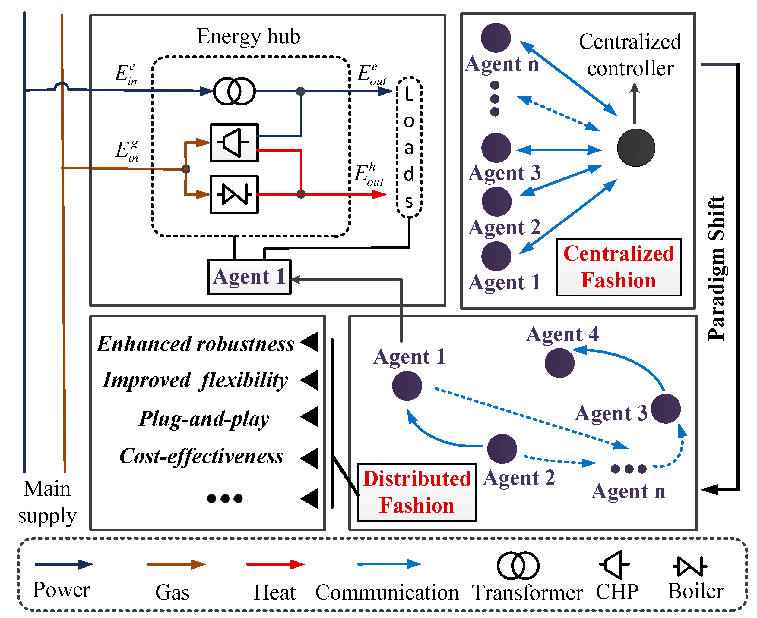
The centralized approaches rely on a powerful central controller to process a huge mass of data and require two-way and high-bandwidth communication to work on the information gathered for the whole system [20,21]. Thus, solutions based on centralized approaches are costly to implement and are prone to single-point failures and modeling errors.
(2)
Despite the plug-and-play and peer-to-peer nature of distributed energy resources, both the physical and associated communication topologies tend to be subject to topology variabilities, which may undermine the efficacy of the centralized approaches [22,23].
As an alternative, the distributed approaches, which have some advantages compared to centralized approaches, e.g., enhanced reliability and robustness [24], fast computation and reduction in communication [25], are more suitable for accommodating a mass of units. Not surprisingly, only a small number of results have been documented. In [26], the authors proposed the concept of smart energy hubs and formulated the interaction among smart energy hubs as a noncooperative game. Therein, a distributed algorithm was introduced to find the Nash equilibrium. Furthermore, the interaction among smart energy hubs was further modeled as an ordinal potential game in [27], where a distributed algorithm was proposed to solve this problem. Considering the autonomy and self-interest among energy hubs, their cooperative interaction was formulated as a bargaining cooperative game in [28], where an alternating direction method of multipliers was applied to find the optimal solutions. It is worth noting that the existing game-theoretic-based distributed approaches can achieve a partial shift from a centralized manner to a distributed manner. However, they also require a cloud computing center, a central price coordinator, or a virtual coordinator to obtain the optimal operations, which may not be regarded as fully distributed methods. Since there are some global supply–demand balance constraints and strong coupling relationship among variables, it is also a challenge to design an algorithm to solve the EMP of multiple energy hubs in a fully distributed manner.
To address these issues, a novel distributed algorithm, referred as the DDC algorithm, is presented. By introducing the consensus concept and designing a new projection operation method, our proposed approach can make the global computation process divided into each energy hub. As a result, each energy hub can locally calculate its optimal operation. Compared to the existing literature, the major contributions of the presented distributed algorithm are summarized as follows:
(1)
By making use of some change of variables, the strongly coupled form between variables in global equality constraints are transformed to the local function and inequality constraints. With this effort, the EMP is formulated as a kind of distributed coupled optimization problem.
(2)
The proposed DDC algorithm, which does not require a price coordinator or a leader to collect global parameters, can solve the EMP in a fully distributed fashion. In contrast to centralized algorithms, the proposed algorithm is more flexible, reliable and robust, etc. To the best knowledge of the authors, there still exist very few papers concerned about solving the EMP for multiple energy hubs in a fully distributed fashion.
(3)
The strong coupling problem, existing in the objective function and constraint limits, can be effectively solved by implementing the proposed DDC algorithm. Moreover, the rigorous optimality and convergence analysis are presented only under strong connectivity conditions, which is more reasonable and general, and possesses less conservatism.
The rest of this paper is organized as follows. In Section 2, the system model and optimal conditions are briefly introduced. In Section 3, some basic knowledge is firstly introduced. Then, the proposed DDC algorithm and the projection operation method are presented. In Section 4, several case studies are presented to show the effectiveness of the proposed DDC algorithm. Section 5 concludes the paper.

2. Problem Formulation

2.1. Energy Hub Model

The energy hub is a concept coupling various energy carriers, such as electricity, gas and heat, etc., which can be converted to various forms of energy to provide diversified loads. Here, for each hub, we consider electricity and natural gas as energy inputs, while electricity and heat are considered as energy outputs. The converter devices consist of a transformer, boiler and CHP unit. The conversion relationship between inputs and outputs is defined as the coupling matrix form given in Appendix A-(a).

2.2. EMP of Multiple Energy Hubs

In this paper, we consider the EMP of interconnected energy hubs to achieve the global optimal energy configuration. Here, the anticipated structure of the multiple energy hubs system is shown in Figure 1. Compared to existing multiple energy hubs systems, it has one important difference, which is the paradigm shift from a traditional centralized manner to a distributed manner. Under this distributed structure, the work of each agent that does not rely on a centralized controller is based only on local communication and calculation to find the optimal operating point and dispatch factor. The considered EMP can be formulated as a distributed optimization problem with a global objective function and a set of constraints.
(1)
Objective: The total objective function is to cooperatively minimize the aggregated energy costs (i.e., the electricity and natural gas consumption costs associated with the individual energy hub) and the emissions penalty from electricity and heat power generation. The mathematical expression of this objective function can be seen in Appendix A-(b).
(2)
Constraints: Energy hubs collectively make decisions on their own subject to global and local constraints. Accordingly, the set of local constraints for each energy hub is listed in Appendix A-(c). Moreover, the global constraints imply the supply–demand balance constraints. Specifically, the total electricity and heat power generation, i.e., i = 1 n E i , o u t e and i = 1 n E i , o u t h , should be equal to the total respective electricity and heat load demands, i.e., i = 1 n l i e and i = 1 n l i h , respectively. In terms of the defined coupling matrix, we can further establish the relationship between the input variables and load demands as follows:
i = 1 n ( η i e e E i , i n e + η i e , c h p ρ i E i , i n g ) = i = 1 n l i e  
i = 1 n ( η i h , c h p ρ i E i , i n g + η i b o i l ( 1 ρ i ) E i , i n g ) = i = 1 n l i h  
It is worth noting that Equations (1a) and (1b) are non-affine constraints caused by the coupled product of variables ρ i and E i , i n g , which is not beneficial to the design of the distributed optimization algorithm. To address this issue, we employ the following change of variables.
E i g , ρ = ρ i E i , i n g ,   E i g , 1 ρ = ( 1 ρ i ) E i , i n g ,   E i , i n e = E i e  
where E i g , ρ and E i g , 1 ρ are the natural gas consumed by CHP unit and boiler, respectively. In this novel coordinate system, the above optimization can be re-written in the following form by some operations.
min   F = i = 1 n ( a i e ( E i e ) 2 + b i e E i e ) + i = 1 n ( α i g ( E i g , ρ ) 2 + β i g ( E i g , 1 ρ ) 2 + γ i g E i g , ρ E i g , 1 ρ + b i g E i g , ρ + b i g E i g , 1 ρ )  
subject to
i = 1 n ( η i e e E i e + η i e , c h p E i g , ρ ) = i = 1 n l i e  
i = 1 n ( η i h , c h p E i g , ρ + η i b o i l E i g , 1 ρ ) = i = 1 n l i h  
and
E i , i n e , m i n E i e E i , i n e , m a x
E i , i n g , m i n E i g , ρ + E i g , 1 ρ E i , i n g , m a x
0 E i g , ρ , 0 E i g , 1 ρ  
where α i g = a i g + ω i e ( η i e , c h p ) 2 + ω i h ( η i h , c h p ) 2 , β i g = a i g + ω i h ( η i b o i l ) 2 and γ i g = 2 a i g + 2 ω i h η i h , c h p η i b o i l .
For convenience, Equations (5b) and (5c) can equally be expressed in the following form
d ˜ i , m E i g , ρ + e ˜ i , m , t E i g , 1 ρ + f ˜ i , m 0 , ( m = 1 , 2 , 3 , 4 )  
Remark 1.
By means of the coordinate transformation in Equation (2), the coupled product form between variables, i.e., ρ i E i , i n g and ( 1 ρ i ) E i , i n g for the global equality constraints, can be transformed into one, i.e., γ i g E i g , ρ E i g , 1 ρ for the local objective function. As a result, the non-affine constraints (1a and 1b) are converged to affine ones, i.e., Equations (4a) and (4b).
Next, the Lagrange multiplier theory can be used to analyze the problem in Equations (3)–(6). Inspired by the Lagrange multiplier theory, a fully distributed algorithm will be introduced in Section 3. The Lagrange function and the corresponding KKT conditions are shown in Appendix A-(d).

3. Distributed Algorithm

3.1. Basic Knowledge

(1)
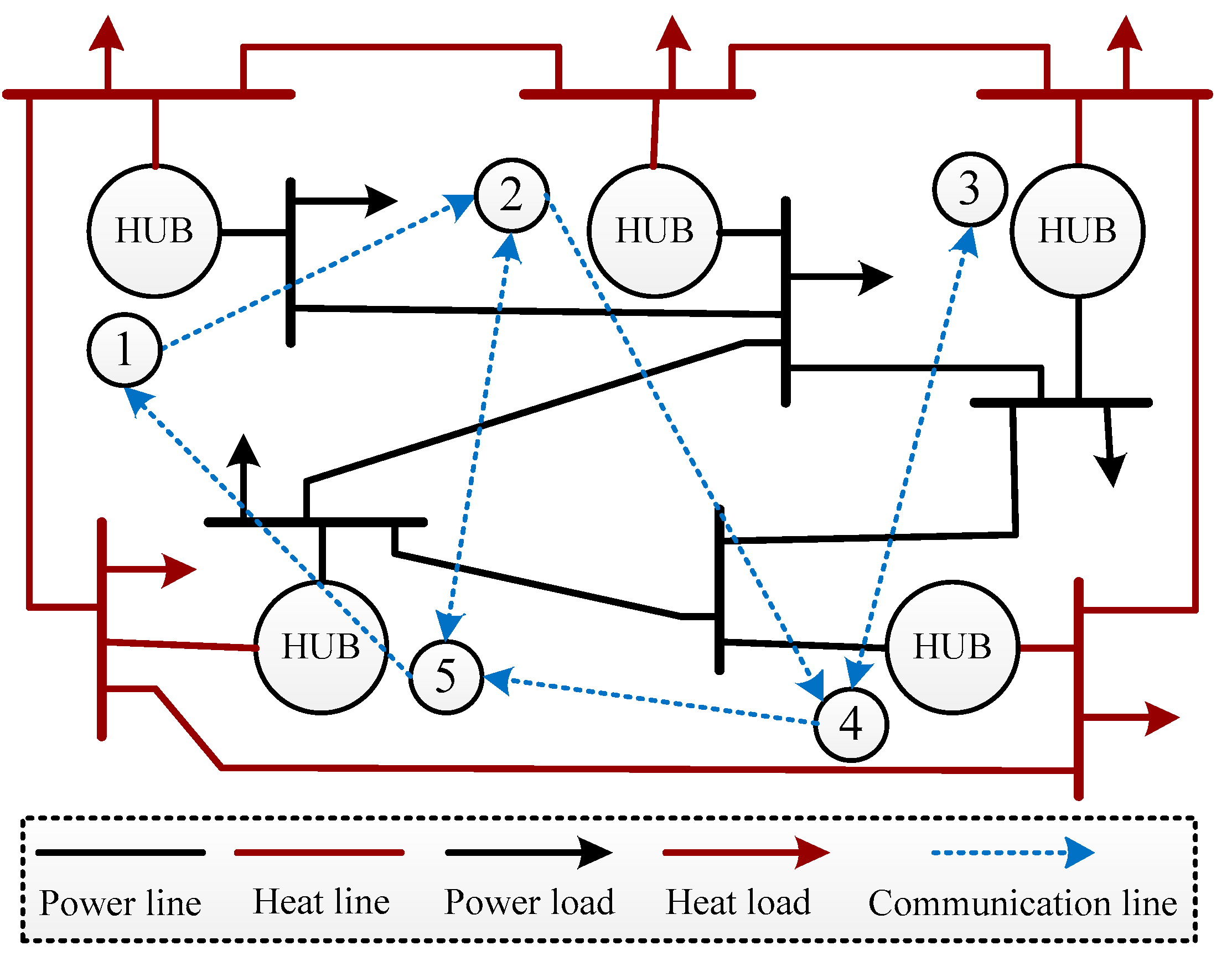
Graph theory: We consider a directed graph G = ( V , E , A ) with a set of vertices V = ( v 1 , v 2 , , v n ) , a set of edges E = ( v i , v j } V × V and an adjacency matrix A = [ a i j ] . The in-neighbors and out-neighbors of ith node are denoted by N i + = { j V { i } : ( j , i ) E } with cardinality d i + and N i = { j V { i } : ( i , j )   E } with cardinality d i , respectively. Each node can receive information from its in-neighbors and send information to its out-neighbors; meanwhile, it can be also assumed to communicate with itself.
(2)
Basic definitions: With regard to problem Equations (3)–(6), there are three variables that need to be calculated. To this aim, we define two strongly regular graphs G1 and G2. The first consists of n nodes, where each node represents the statement related to E i g , 1 ρ . The second is built by dividing each node of graph G1 into two nodes which represent the statements related to E i e and E i g , ρ , respectively. Furthermore, we define two matrices R ¯ = [ r ¯ i , j ] and S ¯ = [ s ¯ i , j ] associated with G 1 ; meanwhile, let r ¯ i , j = 1 / d ¯ i + if j N ¯ i + , r ¯ i , j = 0 if j N ¯ i + , and s ¯ i , j = 1 / d ¯ j if i N ¯ j , s ¯ i , j = 0 if i N ¯ j . It is not difficult to verify that R ¯ is row stochastic and S ¯ is column stochastic. Similarly, we define two matrices R = [ r i , j ] and S = [ s i , j ] for G 2 ; meanwhile, let r i , j = 1 / d i + if j N i + , r i , j = 0 if j N i + , and s i , j = 1 / d j if i N j , s i , j = 0 if i N j .
(3)
Consensus algorithm: Based on the definitions discussed above, we consider two different discrete-time systems—shown in Appendix B-(a)—which will be employed in the design of our proposed algorithm.

3.2. DDC Algorithm without Inequality Constraints

In this section, none of the inequality constraints are taken into consideration; the consideration of inequality constraints will be discussed in the next section. Based on the KKT conditions, we can obtain the relationship between the optimal solutions and the Lagrange multipliers (see Appendix B-(b) for details). This indicates that the optimal E i e , E i g , ρ and E i g , 1 ρ can be obtained if the optimal λe and λg can be calculated. Please note that λe and λg are both global decision variables. In contrast to centralized approaches, there is no central controller to correct the global information to calculate the optimal λe and λg and send the solution to each component. On the contrary, the challenge of this paper is to obtain the optimal λe and λg by using only local information and messages exchanged with neighbors. Meanwhile, λe and λg are interactive with each other. Inspired by the feature of (P1), the basic concept is to establish two different consensus protocols, in which the one is to make all λi,e,p(k) and λi,e,c(k) run a common value and the other is to make all λi,g,c(k) run another common value. Meanwhile a feedback term is added into the corresponding consensus protocol to obtain the optimal λe and λg. Therein, the feedback term uses local estimation of the electricity and heat power mismatches to ensure power and heat supply–demand balances. Then, the designed DDC algorithm, mainly consisting of three parts, is given by:
(1)
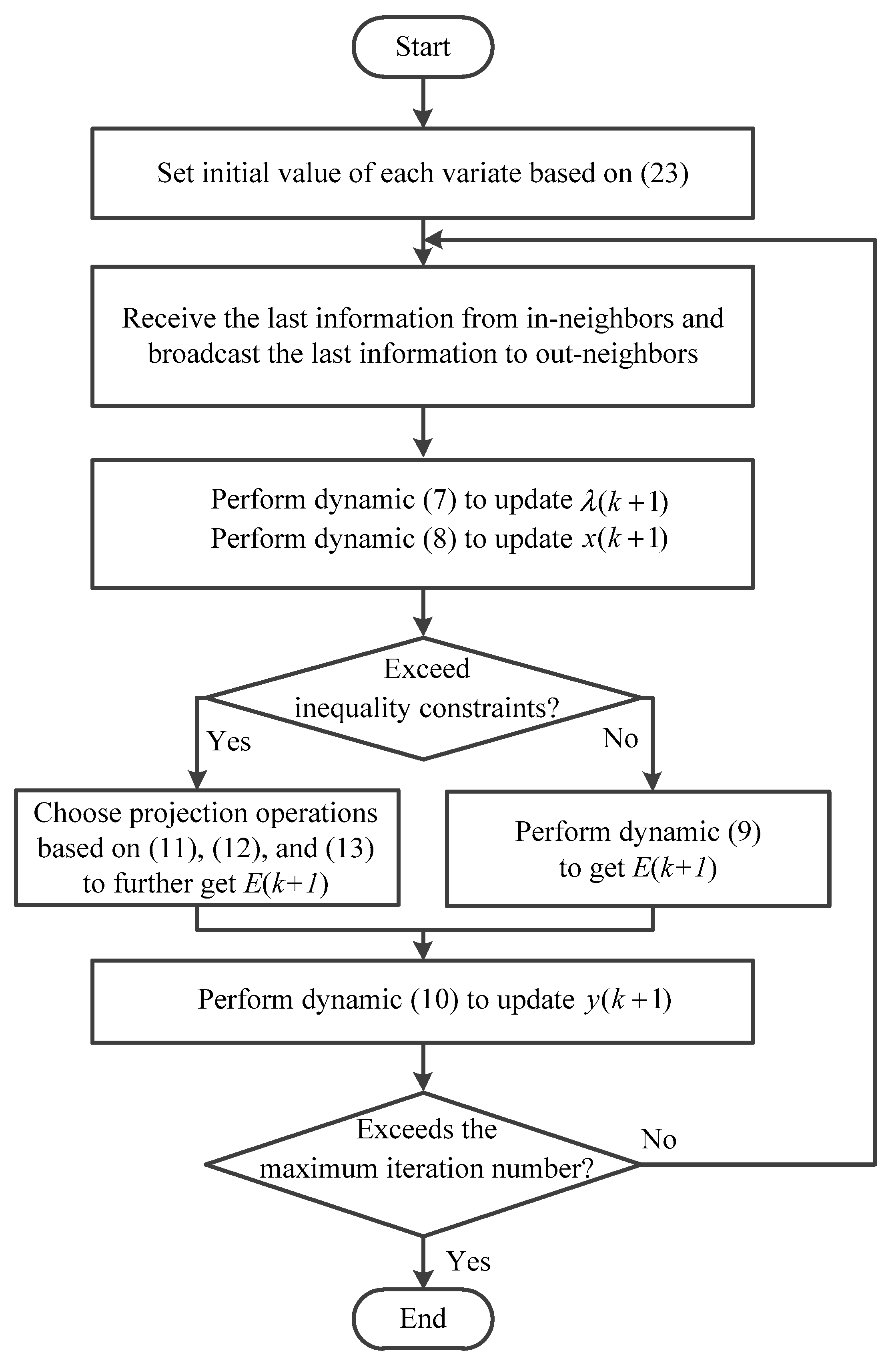
The united updating rules for energy hubs’ coordination to estimate the electricity and heat multipliers are designed for
λ ( k + 1 ) = R   λ ( k ) + η   y ( k )  
where R = [ R 0 0 R ¯ ] , R = [ R p p R p c R c p R c c ] , λ = [ λ e , p T , λ e , c T , λ g , c T ] T and y = [ y e , p T , y e , c T , y g , c T ] T .
(2)
Based on the relationship between the optimal solutions and Lagrange multipliers, the updating rules for energy hubs to estimate the optimal E i e , E i g , ρ and E i g , 1 ρ are designed for
x ( k + 1 ) = A λ ( k + 1 ) + B  
E ( k + 1 ) =   x ( k + 1 )  
where A = [ A p 0 0 0 A p c O p c 0 O h c A h ] , B = [ B p T , B p c T , B h c T ] T , x = [ x e T , x g , ρ T , x g , 1 ρ T ] T and E = [ E e T , E g , ρ T , E g , 1 ρ T ] T . Therein, A p = d i a g ( a ¯ i p ) , A p c = d i a g ( a ¯ i p , c ) , A h c = d i a g ( a ¯ i h , c ) , O p c = d i a g ( o ¯ i p , c ) , O h c = d i a g ( o ¯ i h , c ) , B p T = [ b ¯ i p ] T , B p c T = [ b ¯ i p , c ] T and B h c T = [ b ¯ i h , c ] T .
(3)
Please note that the electricity and heat power supply–demand balance constraints, i.e., Equations (4a) and (4b), are global constraints. Similar to the solving method for λe and λg, the concept of local estimation of the mismatch between demand and total generations, obtained by using only neighbors’ information, is used to solve the two global constraints in a distributed manner. Inspired by the features of (P2), the updating rules for the energy hubs’ coordination to estimate the electricity and heat power mismatches are designed as follows:
y ( k + 1 ) = S y ( k ) ( E ( k + 1 )   E ( k ) )  
where S = [ S 0 0 S ¯ ] , S = [ S p p S p c S c p S c c ] .
With regard to the determination of initializations, they are shown in detail in Appendix B-(c).
Remark 2.
The coordinative updating rules of Equations (7) and (10) show that each component only requires the information received from its in-neighbors to update its corresponding λ and y. In addition, the updating of E is implemented by each energy hub’s own information. Therefore, the DDC algorithm is fully distributed, only requiring local communication and calculation among neighbors, without a central controller.
Lemma 1.
(Perron-Frobenius, [29]) Let P be a primitive nonnegative matrix with left and right eigenvectors w and v , respectively, satisfying P v = v , w T P = w T , and v T w = 1 . Then lim k P k =   v w T .
Theorem 1.
If the problem of Equations (3) and (4) is feasible, there exists a positive value ς such that for all values of 0 < η < ς , the fixed points of the DDC algorithm determined by Equations (7)–(10) satisfy the KKT conditions of optimality.
The proof of Theorem 1 is provided in Appendix C.

3.3. DDC Algorithm with Inequality Constraints

For variable E i e , the corresponding inequality constraints in Equation (5a) can be taken into consideration by introducing the following well-known projection operations.
E i e ( k ) =   { E i , i n e , m i n ,   if   x i e ( k ) < E i , i n e , m i n x i e ( k ) ,   if   E i , i n e , m i n x i e ( k ) E i , i n e , m a x E i , i n e , m i n ,   if   x i e ( k ) > E i , i n e , m a x  
Different from E i e , E i g , ρ and E i g , 1 ρ are coupled by a set of linear inequality constraints, which greatly increases the solving difficulty. To address this issue, the basic concept is to establish a projection operation method that can map the solution without considering inequality constraints onto one point of the feasible operating region determined by Equation (6); meanwhile, the values of this point must satisfy the corresponding KKT conditions. Please note that the new solution may be inside the feasible operating region corresponding to no active constraints, on boundaries corresponding to one active constraint, or at the corner point of boundaries corresponding to two active constraints. Then, according to optimality conditions, we establish the identification conditions for the above three cases, which can be seen in Appendix B-(d).
Furthermore, the projection operations for E i g , ρ and E i g , 1 ρ , to take Equation (6) into account, are given by
E i g , ρ ( k ) =   { x i g , ρ ( k ) ,   if   ( 24 ) satisfied x i , g , ρ ,   if   ( 25 ) satisfied x i , g , ρ ,   if   ( 26 ) satisfied  
E i g , 1 ρ ( k ) = { x i g , 1 ρ ( k ) ,   if   ( 24 ) satisfied x i , g , 1 ρ ,   if   ( 25 ) satisfied x i , g , 1 ρ ,   if   ( 26 ) satisfied  
Theorem 1 can be expanded to solve the problem Equations (3)–(6) by only replacing Equation (9), in Theorem 1, with Equations (11)–(13). For clarity, the flowchart of the proposed DDC algorithm is summarized in Figure 2.
Remark 3.
The coupled variables problem can be effectively solved by implementing the proposed DDC algorithm. Firstly, we express E i g , ρ and E i g , 1 ρ without inequality constraints as the linearcombination of λ e and λ g . Then, the directcalculation of E i g , ρ and E i g , 1 ρ can be transformed into theindirect calculation of λ p and λ h , which can effectively handle the coupled variables existing in the objective function. Furthermore, along with the KKT conditions and the solution without inequality constraints, the proposed projection operation method maps infeasible values into the feasible operation region, which can further effectively handle the coupled variables existing within the inequality constraint limits.

4. Application Examples

In this section, several simulations have been studied to verify the effectiveness of the proposed algorithm. The first case is used to show the effectiveness of the proposed DDC algorithm via comparison to a centralized algorithm. The second case shows the performance of the proposed algorithm under time-varying demand. The third case demonstrates the plug and play properties of the proposed algorithm. The configuration and communication structures of the test system with five energy hubs are shown in Figure 3. The energy transformer efficiencies ηee, ηe,chp, ηh,chp and ηboil are selected as 0.98, 0.35, 0.4 and 0.9, respectively. The cost parameters and constraints of each hub are listed in Table 1.

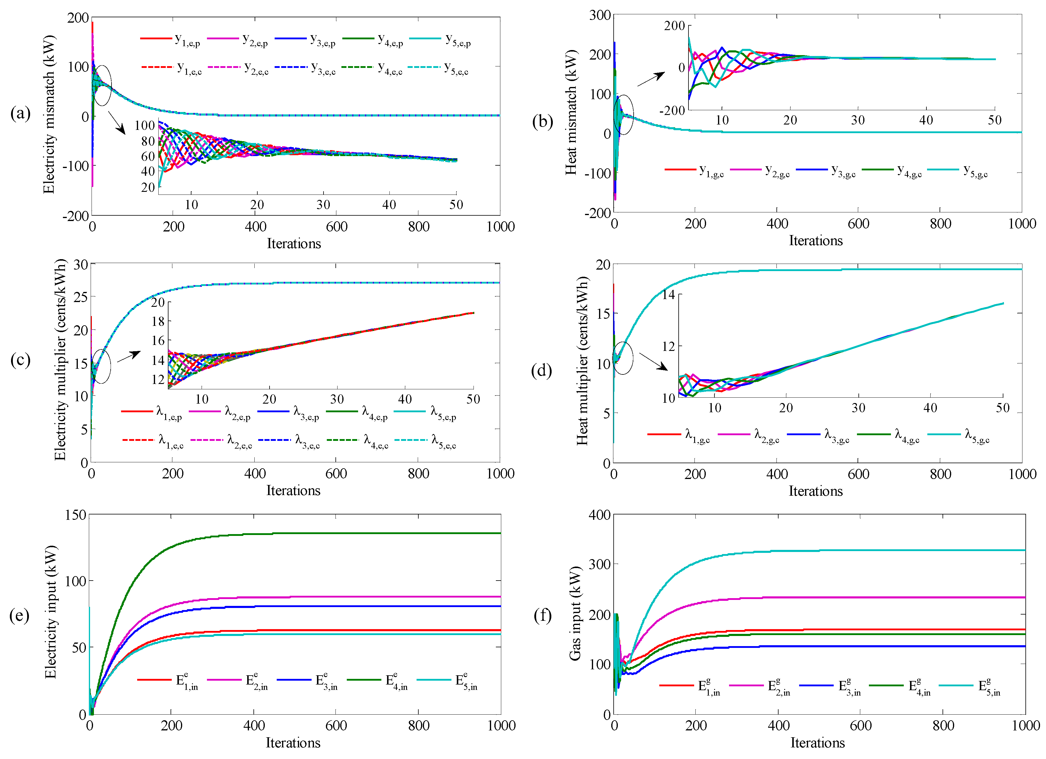
4.1. Comparison with Centralized Algorithm

This case study focuses on verifying the effectiveness of the proposed DDC algorithm by comparing it to the centralized algorithm [30]. The power and heat load demands for each power and heat load are initialized at 150 kW and 140 kW, respectively. By running the DDC algorithm, the estimated electricity and heat Lagrangian multipliers, mismatches and energy inputs are shown in Figure 4. After the algorithm converges, it can be observed that the electricity multipliers converge to a common value, λ p = 27.0354 cents/kWh, and the heat multipliers converge to another value, λ h = 19.3652 cents/kWh; meanwhile, the electricity and heat mismatches converge to zero, which means that the power and heat supply–demand equality constraints are satisfied. In addition, the final electricity and gas inputs of each hub are within their corresponding inequality constraints, as shown in Table 2. Therefore, the optimization goal has been fulfilled. Furthermore, the performance of the proposed DDC algorithm is compared with a centralized algorithm. The simulation results provided by the two approaches are shown in Table 2. It can be seen that all of the solutions are very similar, which also verifies the effectiveness of the proposed algorithm.

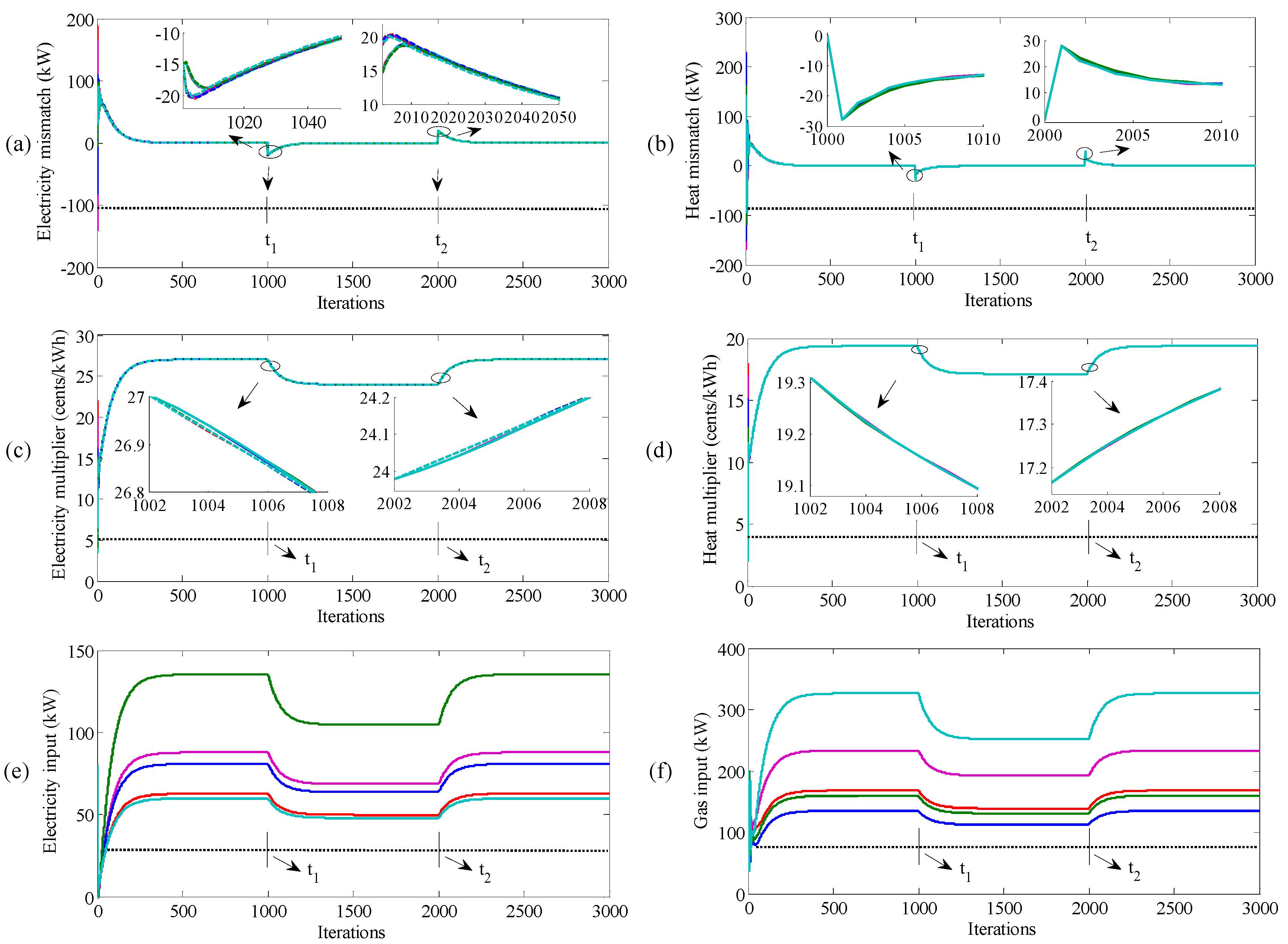
4.2. Time-Varying Demand

This case study focuses on testing the capability of the proposed DDC algorithm to handle changes in load demand. The initial conditions are the same as those in case study 1, and the load demand changes 2 times during the simulation. At t1 (k = 1000), the total power and heat load demands decrease by 20%, while at t2 (k = 2000), they are increased by 20%. The simulation results are shown in Figure 5. It can be observed from Figure 5a,b that neither the electricity nor heat mismatch can be maintained at a zero state after t1, because of the reduced power and heat load demands. By continually running the proposed DDC algorithm, each energy hub gradually reduces its electricity and gas inputs to meet the new supply-demand balance, as seen in Figure 5e,f; meanwhile, the electricity and heat multipliers decrease in response to the change seen in Figure 5c,d. After about 300 iterations, i.e., at k = 1300, the electricity and heat mismatches converge to zero again, and not only the electricity Lagrangian multipliers, but also the heat Lagrangian multipliers, converge to new common values. This implies that the new supply-demand balance and the optimization goal have been fulfilled. Furthermore, the balance is broken at t2 due to the increased load demands. From Figure 5a–f, it can be seen that after about 300 iterations, i.e., at k = 1300, the electricity and heat mismatches go to zero, both the electricity and heat multipliers increase and converge to new optimal values, and each hub increases its energy input to compensate for part of the increased load, finally converging to the new solutions. Based on the aforementioned discussion, it can be concluded that the proposed DDC algorithm can respond automatically to converge to new optimal solutions after each load change. This also means that the proposed DDC algorithm works properly under time-varying demand.

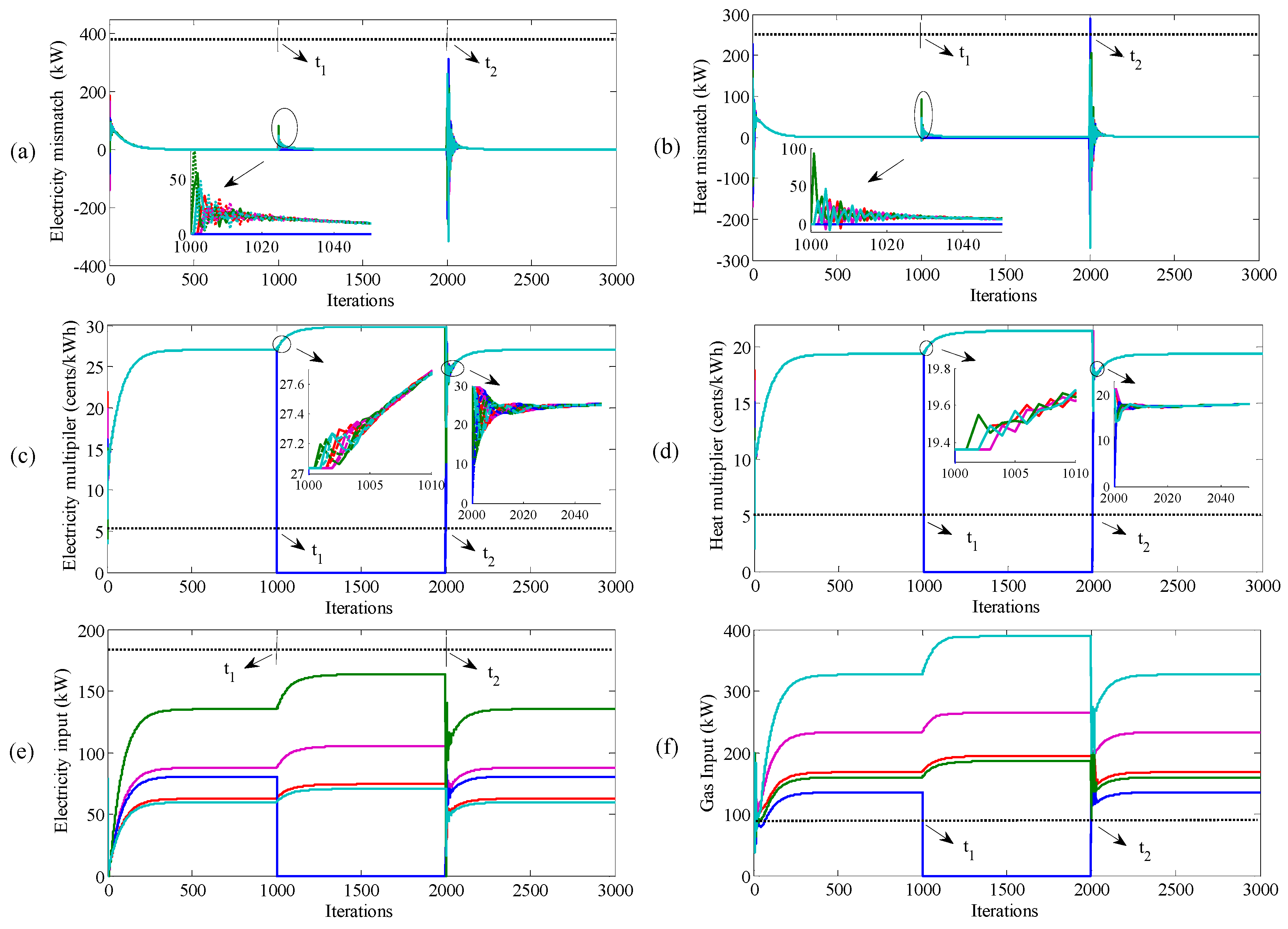
4.3. Plug and Play Capability

This case study focuses on testing the plug and play performance of the proposed algorithm. The initial conditions are the same as those in case study 1. At t1 (k = 1000), hub3 is removed from the test system and the variables related to them are set to zero. As a result of this change, the original balance is broken, and the electricity and heat mismatches go to a non-zero state, as seen in Figure 6a,b. By continually running the proposed DDC algorithm, it can be observed from Figure 6c–f that the remaining energy hubs have to increase their electricity and gas inputs to generate more electricity and heat to further compensate for the amount of electricity and heat previously generated by hub3; the corresponding electricity and heat Lagrangian multipliers increase, as well, to meet this change. After about 300 iterations, i.e., at k = 1300, the electricity and heat mismatches converge to zero again; meanwhile, the electricity and heat Lagrangian multipliers, as well as the electricity and heat inputs, converge to their corresponding optimal values. As a result, the new supply–demand balance can be satisfied after removing hub3. Then, at t2 (k = 2000), hub3 is plugged back into the system again. Of course, hub3 gradually increases its electricity and heat generation, while the others decrease their generations to accommodate for hub3. After about 300 iterations, i.e., at k = 2300, it can be seen from Figure 5a–f that the algorithm converges to the new optimal solution in response to the new topological change. Additionally, the final convergence values for all variables are the same as those prior to disconnection. Therefore, the results clearly show that our proposed algorithm can provide good plug and play capability.

5. Conclusions

In this paper, we have presented a novel DDC algorithm to solve the EMP for multiple energy hubs, which is formulated as a class of distributed coupled optimization problem by properly converting some system coordinates. The consensus concept in multiagent systems has been explored and embedded in the design of our distributed algorithm. With this effort, the total computation process can be completely assigned to each individual energy hub without the requirements of a cloud computing center, a central price coordinator or a virtual coordinator. Thus, our proposed algorithm can improve the existing game-theoretic-based distributed approaches, which further solves the EMP for multiple energy hubs in a fully distributed fashion. In addition, a novel projection operation method has also been proposed to address the issue of coupled variables existing in the objective function and constraint limits. Furthermore, we have proved that the proposed algorithm can converge to the optimal solution under strong connectivity conditions only. In the simulation part, several examples were presented to illustrate the effectiveness of the DDC algorithm and to demonstrate the correctness of the theoretical result. In future work, the rate of convergence and underlying energy flow control will be studied.

Author Contributions

Y.-S.L. conceived the idea for the manuscript and wrote the manuscript with input from T.-Y.L., B.-N.H. and J.-G.Z.

Funding

This research was funded by the National Natural Science Foundation of China (NSFC) grant number 61433004, the NSFC grant number 61621004, the NSFC grant number 61603085 and the National Natural Science Foundation of Liaoning Province grant number 201601020.

Acknowledgments

This work was supported in part by the National Natural Science Foundation of China (NSFC) under Grant No. 61433004, the NSFC under Grant No. 61621004, the NSFC under Grant No. 61603085, and the National Natural Science Foundation of Liaoning Province under Grant No. 201601020.

Conflicts of Interest

The authors declare no conflict of interest.

Nomenclature

EMPEnergy management problem
DDCDistributed double-consensus
CHPCombined heat and power
KKTKarush-Kuhn-Tucker
i , j energy hub indices
nNumber of energy hubs
mLinear inequality constraint indices
E i n e , E i n g Inputs of electricity and natural gas powers
E i , i n e , m i n , E i , i n e , m a x Lower and upper bounds of E i , i n e
E i , i n g , m i n , E i , i n g , m a x Lower and upper bounds of E i , i n g
E o u t e , E o u t g Outputs of electricity and heat powers
η e e , η e , c h p , η h , c h p , η b o i l The transformer efficiencies of transformer, CHP unit from gas to electricity, CHP unit from gas to heat and boiler
ρ Dispatch factor
C i ( E i , i n e ) , C i ( E i , i n g ) Electricity and natural gas cost functions
W i ( η , E i , i n g ) Penalty function
a i e , a i g , b i e , b i g Cost coefficients
ω i e , ω i h penalty coefficients
l i e , l i h Local electricity and natural gas loads connected to ith energy hub
d ˜ i , m , e ˜ i , m , f ˜ i , m Coefficients of mth linear inequality constraint for variables E i g , ρ and E i g , 1 ρ
λ e and λ g Electricity and heat multipliers for the equality constraints
u i e , m i n , u i e , m a x , u i , m g Lagrangian multiplier for inequality constraints
χ i , χ ˜ i State variables of agent i
w T Normalized left eigenvector of R associated with the eigenvalue 1
χ Column stack vector of χ i
λ i , e , p ( k ) , λ i , e , c ( k ) Estimated electricity multipliers
λ i , g , c ( k ) Estimated heat multiplier
y i , e , p ( k ) , y i , e , c ( k ) Estimated electricity power mismatches
y i , g , c ( k ) Estimated heat power mismatch
E i e ( k ) , E i g , ρ ( k ) , E i g , 1 ρ ( k ) Estimated of optimal E i e , E i g , ρ and E i g , 1 ρ
λ e , p , λ e , c , λ g , c , y e , p , y e , c , y g , c Column stack vectors form of λ i , e , p , λ i , e , c , λ i , g , c , y i , e , p , y i , e , c and y i , g , c
x e , x g , ρ , x g , 1 ρ , E e , E g , ρ , E g , 1 ρ Column stack vectors of x i e , x i g , ρ , x i g , 1 ρ , E i e , E i g , ρ and E i g , 1 ρ

Appendix A. Constraints and Optimality Conditions

(a)
The conversion relationship between inputs and outputs can be expressed as the following coupling matrix form,
[ E o u t e E o u t h ] = [ η e e η e , c h p ρ 0 η h , c h p ρ + η b o i l ( 1 ρ ) ] [ E i n e E i n g ]  
where the dispatch factor ρ [ 0 , 1 ] is introduced to specify the share of natural gas by the CHP unit and boiler.
(b)
The total objective function of the EMP for multiple energy hubs is modeled as the following form,
min   F = i = 1 n ( C i ( E i , i n e ) + C i ( E i , i n g ) + W i ( η , E i , i n g ) )  
where
{ C i ( E i , i n e ) = a i e ( E i , i n e ) 2 + b i e E i , i n e C i ( E i , i n g ) = a i g ( E i , i n g ) 2 + b i g E i , i n g W i ( η , E i , i n g ) = ω i e ( η i e , c h p ρ i E i , i n g ) 2 + ω i h ( η i h , c h p ρ i E i , i n g + η i b o i l ( 1 ρ i ) E i , i n g ) 2  
(c)
The local constraints arise from the limitations of the energy hubs’ capability and the dispatch factors, which are expressed as
E i , i n e , m i n E i , i n e E i , i n e , m a x  
E i , i n g , m i n E i , i n g E i , i n g , m a x  
0 ρ i 1  
(d)
The Lagrange function for problem (3)–(6) is expressed as the following equation:
L = F λ e [ i = 1 n ( η i e e E i e + η i e , c h p E i g , ρ ) i = 1 n l i e ] λ g [ i = 1 n ( η i h , c h p E i g , ρ + η i b o i l E i g , 1 ρ ) i = 1 n l i h ] i = 1 n u i e , m i n ( E i e E i , i n e , m i n ) i = 1 n u i e , m a x ( E i , i n e , m a x E i e ) i = 1 n m = 1 4 u i , m g ( d ˜ i , m E i g , ρ + e ˜ i , m , t E i g , 1 ρ + f ˜ i , m ) ,  
The optimal operating point is determined by the following KKT conditions:
{ F / E i e = λ e η i e e + u i e , m i n u i e , m a x F / E i g , ρ = λ e η i e , c h p + λ g η i h , c h p + m = 1 4 u i , m g d ˜ i , m F / E i g , 1 ρ = λ g η i b o i l + m = 1 4 u i , m g e ˜ i , m u i e , m i n ( E i e E i , i n e , m i n ) = 0 , u i e , m a x ( E i , i n e , m a x E i e ) = 0 u i , m g ( d ˜ i , m E i g , ρ + e ˜ i , m , t E i g , 1 ρ + f ˜ i , m ) = 0 u i e , m i n 0 , u i e , m a x 0 , u i , m g 0 ,
and Equation (4a) along with Equation (4b).

Appendix B. Consensus Algorithm, Initializations and Projection Conditions

(a)
The two different discrete-time systems considered are as follows:
( P 1 )         χ i ( k + 1 ) = j N i + r i , j χ j ( k )  
( P 2 )         χ ˜ i ( k + 1 ) = j N i + s i , j χ ˜ j ( k )  
Since R is row stochastic, P1 forms the first-order consensus protocol. Each node reaches the final common value χ i ( ) = w T χ ( 0 ) . Since S is column stochastic, the summation of all state variables is a constant, i.e., χ ˜ i ( k ) = χ ˜ i ( 0 ) .
(b)
We let u i e , m i n = u i e , m a x = u i , m g = 0 . Then, according to the first three equations of Equation (12), the optimal solution of E i e , E i g , ρ and E i g , 1 ρ of each energy hub can be determined by the unique Lagrange multipliers λe and λe, given by
{ E i e = a ¯ i p λ e b ¯ i p E i g , ρ = a ¯ i p , c λ e o ¯ i p , c λ g b ¯ i p , c E i g , 1 ρ = a ¯ i h , c λ g o ¯ i h , c λ e b ¯ i h , c  
where a ¯ i p = η i e e / 2 a i e , b ¯ i p = b i e / 2 a i e , a ¯ i p , c = 2 β i g η i e , c h p / ϑ , o ¯ i p , c = ( γ i g η i b o i l 2 β i g η i h , c h p ) / ϑ , b ¯ i p , c = ( 2 β i g b i g γ i g b i g ) / ϑ , o ¯ i h , c = γ i g η i e , c h p / ϑ , a ¯ i h , c = ( 2 α i g η i b o i l γ i g η i h , c h p ) / ϑ , b ¯ i h , c = ( 2 α i g b i g , γ i g b i g ) / ϑ , and ϑ = 4 α i g β i g ( γ i g ) 2 .
(c)
E i e ( 0 ) , E i g , ρ ( 0 ) and E i g , 1 ρ ( 0 ) can be designed as any admissible values, and the other variables are initialized as
{ y i , e , p ( 0 ) = l i e / 2 E i e ( 0 ) y i , e , c ( 0 ) = l i e / 2 E i g , ρ ( 0 ) y i , g , c ( 0 ) = l i h E i g , 1 ρ ( 0 ) λ i , e , p ( 0 ) = λ i , e , c ( 0 ) = λ i , g , c ( 0 ) = 0  
(d)
To map the infeasible values into the feasible operating region, the cases for no active constraints, one active constraint and two active constraints are separately discussed to further give the corresponding identification conditions as follows:
(1)
None of the constraints are active constraints, i.e., the optimal solutions before and after considering the inequality constraints have the same values. The identification condition of this case is if x i g , ρ ( k ) and x i g , 1 ρ ( k ) satisfy
d ˜ i , m x i g , ρ ( k ) + e ˜ i , m x i g , 1 ρ ( k ) + f ˜ i , m > 0  
then there are no active constraints; otherwise, the optimal solution belongs to another case.
(2)
Only one inequality constraint is an active constraint. Let represent any one inequality equation. The identification condition of this case is that if there exist solutions x i , , g , ρ , x i , , g , 1 ρ and u i , g 0 satisfying
{ 2 α i g x i , g , ρ + b i g + γ i g x i , g , 1 ρ = λ i , e , c ( k ) η i e , c h p                                   + λ i , g , c ( k ) η i h , c h p + u i , g d ˜ i , 2 β i g x i , g , 1 ρ + b i g + γ i g x i , g , ρ = λ i , g , c ( k ) η i b o i l + u i , g e ˜ i , d ˜ i , x i , g , ρ + e ˜ i , x i , g , 1 ρ + f ˜ i , = 0 d ˜ i , m x i , m g , ρ + e ˜ i , m x i , m g , 1 ρ + f ˜ i , m > 0             ( m = { 1 , , 4 } )
then is the only active constraint; otherwise, the optimal solution belongs to another case.
(3)
Two inequality constraints are active constraints. In this case, let and represent two adjacent constraints (e.g., 2 and 3) and the corner point determined by them be defined as ( x i , , g , ρ , x i , , g , 1 ρ ) . The identification condition of this case is that if there exist solutions u i , g 0 and u i , g 0 satisfying
{ 2 α i g x i , g , ρ + b i g + γ i g x i , g , 1 ρ = λ i , e , c ( k ) η i e , c h p                                   + λ i , g , c ( k ) η i h , c h p + u i , g d ˜ i , + u i , g d ˜ i , 2 β i g x i , g , 1 ρ + b i g + γ i g x i , g , ρ = λ i , g , c ( k ) η i b o i l                                   + u i , g e ˜ i , + u i , g e ˜ i ,  
then, and are the two active constraints; otherwise, the optimal solution belongs to another case.

Appendix C. Proof of Theorem 1

M = [ R p p R p c 0 0 0 0 R c p R c c 0 0 0 0 0 0 R ¯ 0 0 0 A p ( I R p p ) A p R p c 0 S p p S p c 0 A p c R c p A p c ( I R c c ) O p c ( I R ¯ ) S c p S c c 0 O h c R c p O h c ( I R c c ) A h c ( I R ¯ ) 0 0 S ¯ ] ,  
Δ = [ 0 0 0 I 0 0 0 0 0 0 I 0 0 0 0 0 0 I 0 0 0 A p 0 0 0 0 0 0 A p c O p c 0 0 0 0 O h c A h c ] , V = [ V 1 T V 1 T V 1 T V 1 T ] T = [ 0 0 1 0 0 0 1 0 0 0 0 1 v p 0 κ p p v p κ p c v p v c 0 κ p p v c κ p c v c 0 v ¯ c κ c p v ¯ c κ h h v ¯ c ] ,  
W T [ W 1 T W 1 T W 1 T W 1 T ] = [ 1 T A p 1 T A p c 1 T O p c 1 T 1 T 0 T 0 T 1 T O h c 1 T A h c 0 T 0 T 1 T w p T w c T 0 T 0 T 0 T 0 T 0 T 0 T w ¯ c T 0 T 0 T 0 T ] , Q = [ 0 0 0 0 0 0 0 0 1 0 κ p p κ p c 0 1 κ c p κ h h ]  
The eigenvalue perturbation approach is employed to analyze the convergence properties of the presented algorithm. Along with Equations (7)–(10), we get
Θ ( k + 1 ) = ( M + η Δ ) Θ ( k )  
where Θ = [ λ e , p T , λ e , c T , λ g , c T , y e , p T , y e , c T , y g , c T ] T .
Due to the definition of R, R ¯ , S and S ¯ , it is not difficult to verify that R, R ¯ , S and S ¯ are all primitive with the maximum eigenvalue 1. Based on Lemma 1, there exist four vectors w T , v , w ¯ T and v ¯ , satisfying w T R = w T , S v = v , w ¯ T R ¯ = w ¯ T and S ¯ v ¯ = v ¯ meanwhile w T 1 = 1 , 1 T v = 1 , w ¯ T 1 = 1 and 1 T v ¯ = 1 . Therein, 1 denotes a vector with all its elements being 1. To facilitate the analysis, w T and v are expressed in the corresponding block vectors form, i.e., w T = [ w p T , w c T ] and v = [ v p T , v c T ] T . Furthermore, M is a lower block triangular matrix whose eigenvalues are the union of R, R ¯ , S and S ¯ , so M has four maximum eigenvalues ψ 1 = ψ 2 = ψ 3 = ψ 4 = 1 while the other eigenvalues lie in the open unit disk on the complex plane. Then, the eigenvalue perturbation approach is used to analyze the eigenvalue changing of M after perturbing by η Δ . Let κ p p = a ¯ p + a ¯ p , c , κ p c = o ¯ p , c , κ c p = o ¯ h , c v and κ h h = a ¯ h , c . On this basis, V and WT are defined as the right and left eigenvectors of M, respectively. In this way, W T V = I . Then, along with Δ, V and WT, the matrix W T Δ V can be mathematically represented as follows:
W T Δ V = Q  
Since the object function is a convex function, it is not difficult to verify κ p c κ c p < κ h h κ p p . According to Q, we have the four eigenvalues of W T Δ V satisfying d ψ 1 / d η = d ψ 2 / d η = 0 , d ψ 3 / d η < 0 and d ψ 4 / d η < 0 , which means ψ1 and ψ2 do not change against η , and ψ3 and ψ4 become smaller when η > 0 . Thus, there exists an upper boundary ς such that 0 < η < ς . Except for ψ 1 = ψ 2 = 1 , the remaining eigenvalues lie in the open unit disk. Moreover, it can be verified that [ 1 T , 1 T , 0 T , 0 T , 0 T , 0 T , 0 T ] T and [ 0 T , 0 T , 1 T , 1 T , 0 T , 0 T ] T are the two independent eigenvectors of M corresponding to ψ1 and ψ2, respectively. That means that, as k , all of y i , e , p ( k ) , y i , e , c ( k ) and y i , g , c ( k ) converge to 0, i.e., the electricity and heat power supply–demand balance constraints are satisfied. At the same time, λ i , e , p ( k ) , λ i , e , c ( k ) converge to a common value, while λ i , g , c ( k ) converges to another common value. Therefore, the optimality conditions (KKT conditions of optimality) are satisfied.

References

  1. Han, R.; Meng, L.; Guerrero, J.M.; Vasquez, J.C. Distributed nonlinear control with event-triggered communication to achieve current-sharing and voltage regulation in DC microgrids. IEEE Trans. Power Electron. 2018, 33, 6416–6433. [Google Scholar] [CrossRef]
  2. Zhang, H.; Li, Y.; Gao, D.W.; Zhou, J. Distributed optimal energy management for energy internet. IEEE Trans. Ind. Inform. 2017, 13, 3081–3097. [Google Scholar] [CrossRef]
  3. Geidl, M.; Andersson, G. Optimal power flow of multiple energy carriers. IEEE Trans. Power Syst. 2007, 22, 145–155. [Google Scholar] [CrossRef]
  4. Krause, T.; Andersson, G.; Frohlich, K.; Alfredo, V. Multiple-energy carriers: Modeling of production, delivery, and consumption. Proc. IEEE 2011, 99, 15–27. [Google Scholar] [CrossRef]
  5. Tronchin, L.; Manfren, M.; Nastasi, B. Energy efficiency, demand side management and energy storage technologies—A critical analysis of possible paths of integration in the built environment. Renew. Sustain. Energy Rev. 2018, 95, 341–353. [Google Scholar] [CrossRef]
  6. Berardi, U.; Tronchin, L.; Manfren, M.; Nastasi, B. On the effects of variation of thermal conductivity in buildings in the italian construction sector. Energies 2018, 11, 872. [Google Scholar] [CrossRef]
  7. Tronchin, L.; Tommasino, M.C.; Fabbri, K. On the “cost-optimal levels” of energy performance requirements and its economic evaluation in Italy. Int. J. Sustain. Energy Plan. Manag. 2014, 3, 49–62. [Google Scholar]
  8. Tronchin, L.; Manfren, M.; Tagliabue, L.C. Optimization of building energy performance by means of multi-scale analysis–Lessons learned from case studies. Sustain. Cities Soc. 2016, 27, 296–306. [Google Scholar] [CrossRef]
  9. Paterakis, N.G.; Erdinç, O.; Catalão, J.P.S. An overview of demand response: Key-elements and international experience. Renew. Sustain. Energy Rev. 2017, 69, 871–891. [Google Scholar] [CrossRef]
  10. Parisio, A.; Del Vecchio, C.; Vaccaro, A. A robust optimization approach to energy hub management. Int. J. Electr. Power Energy Syst. 2012, 42, 98–104. [Google Scholar] [CrossRef]
  11. Rastegar, M.; Fotuhi-Firuzabad, M. Load management in a residential energy hub with renewable distributed energy resources. Energy Build. 2015, 107, 234–242. [Google Scholar] [CrossRef]
  12. Adamek, F.; Arnold, M.; Andersson, G. On decisive storage parameters for minimizing energy supply costs in multicarrier energy systems. IEEE Trans. Sustain. Energy 2013, 5, 102–109. [Google Scholar] [CrossRef]
  13. Moeini-Aghtaie, M.; Dehghanian, P.; Fotuhi-Firuzabad, M.; Ali, A. Multiagent genetic algorithm: An online probabilistic view on economic dispatch of energy hubs constrained by wind availability. IEEE Trans. Sustain. Energy 2014, 5, 699–708. [Google Scholar] [CrossRef]
  14. Rastegar, M.; Fotuhi-Firuzabad, M.; Zareipour, H.; Moein, M.-A. A probabilistic energy management scheme for renewable-based residential energy hubs. IEEE Trans. Smart Grid 2017, 8, 2217–2227. [Google Scholar] [CrossRef]
  15. Beigvand, S.D.; Abdi, H.; Scala, M.L. A general model for energy hub economic dispatch. Appl. Energy 2017, 190, 1090–1111. [Google Scholar] [CrossRef]
  16. Shabanpour-Haghighi, A.; Seifi, A.R. Energy flow optimization in multicarrier systems. IEEE Trans. Ind. Inform. 2015, 11, 1067–1077. [Google Scholar] [CrossRef]
  17. Shao, C.; Wang, X.; Shahidehpour, M.; Wang, X.; Wang, B. An MILP-based optimal power flow in multicarrier energy systems. IEEE Trans. Sustain. Energy 2017, 8, 239–248. [Google Scholar] [CrossRef]
  18. Moeini-Aghtaie, M.; Farzin, H.; Fotuhi-Firuzabad, M.; Reza, A. Generalized analytical approach to assess reliability of renewable-based energy hubs. IEEE Trans. Power Syst. 2017, 32, 368–377. [Google Scholar] [CrossRef]
  19. Zhang, X.; Che, L.; Shahidehpour, M.; Alabdulwahab, A.S. Reliability-based optimal planning of electricity and natural gas interconnections for multiple energy hubs. IEEE Trans. Smart Grid 2017, 8, 1658–1667. [Google Scholar] [CrossRef]
  20. Liu, N.; Wang, J. Energy sharing for interconnected microgrids with a battery storage system and renewable energy sources based on the alternating direction method of multipliers. Appl. Sci. 2018, 8, 590. [Google Scholar] [CrossRef]
  21. Li, Y.; Zhang, H.; Liang, X.; Huang, B. Event-triggered based distributed cooperative energy management for multi-energy systems. IEEE Trans. Ind. Inf. 2018. [Google Scholar] [CrossRef]
  22. Han, R.; Meng, L.; Ferrari-Trecate, G.; Coelho, E.A.A.; Vasquez, J.C.; Guerrero, J.M. Containment and consensus-based distributed coordination control to achieve bounded voltage and precise reactive power sharing in islanded ac microgrids. IEEE Trans. Ind. Appl. 2017, 53, 5187–5199. [Google Scholar] [CrossRef]
  23. Li, Y.; Zhang, H.; Han, J.; Sun, Q. Distributed multi-agent optimization via event-triggered based continuous-time newton-raphson algorithm. Neurocomputing 2018, 275, 1416–1425. [Google Scholar] [CrossRef]
  24. Lao, M.; Tang, J. Cooperative multi-UAV collision avoidance based on distributed dynamic optimization and causal analysis. Appl. Sci. 2017, 7, 83. [Google Scholar] [CrossRef]
  25. Varagnolo, D.; Zanella, F.; Cenedese, A.; Gianluigi, P.; Luca, S. Newton-raphson consensus for distributed convex optimization. IEEE Trans. Autom. Control 2016, 61, 994–1009. [Google Scholar] [CrossRef]
  26. Xie, X.; Yue, D.; Peng, C. Relaxed real-time scheduling stabilization of discrete-time takagi-sugeno fuzzy systems via a alterable-weights-based ranking switching mechanism. IEEE Trans. Fuzzy Syst. 2018. [Google Scholar] [CrossRef]
  27. Bahrami, S.; Sheikhi, A. From demand response in smart grid toward integrated demand response in smart energy hub. IEEE Trans. Smart Grid 2016, 7, 650–658. [Google Scholar] [CrossRef]
  28. Fan, S.; Li, Z.; Wang, J.; Piao, L.; Qian, A. Cooperative economic scheduling for multiple energy hubs: A bargaining game theoretic perspective. IEEE Access 2018, 6, 27777–27789. [Google Scholar] [CrossRef]
  29. Horn, R.A.; Johnson, C.R. Matrix Analysis; Cambridge University Press: Cambridge, UK, 1985. [Google Scholar]
  30. Roldán-Blay, C.; Escrivá-Escrivá, G.; Roldán-Porta, C.; Carlos, Á.-B. An optimisation algorithm for distributed energy resources management in micro-scale energy hubs. Energy 2017, 132, 126–135. [Google Scholar] [CrossRef]
Figure 1. Structure of a multiple energy hubs system.
Applsci 08 01412 g001
Figure 2. Flowchart of the proposed DDC algorithm.
Applsci 08 01412 g002
Figure 3. Structure of multiple energy hub system.
Applsci 08 01412 g003
Figure 4. Comparison with centralized algorithm: (a) the electricity mismatch; (b) the heat mismatch; (c) the electricity multiplier; (d) the heat multiplier; (e) electricity input; (f) gas input.
Applsci 08 01412 g004
Figure 5. Time-varying demand: (a) the electricity mismatch; (b) the heat mismatch; (c) the electricity multiplier; (d) the heat multiplier; (e) electricity input; (f) gas input.
Applsci 08 01412 g005
Figure 6. Plug and play capability: (a) the electricity mismatch; (b) the heat mismatch; (c) the electricity multiplier; (d) the heat multiplier; (e) electricity input; (f) gas input.
Applsci 08 01412 g006
Table 1. Parameters of the test system.
NumberHub1Hub2Hub3 Hub4Hub5
a e   0.120.080.090.050.13
b e 12.013.012.513.511.5
a g 0.0330.0230.0420.0330.012
b g 5.86.05.56.38.6
ω e 0.0110.0120.0090.0120.008
ω h 0.0210.0230.0310.0250.026
E e , m i n 00000
E e , m a x 200150175210200
E g , m i n 00000
E e , m a x 200275150175375
Table 2. Comparison with centralized algorithm.
Number DDC AlgorithmCentralized Algorithm
E e   E g   E e   E g  
Hub162.6477168.267062.7895168.2715
Hub287.7216233.460187.7325233.4569
Hub380.7525135.310280.7861135.3133
Hub4135.3545159.9385135.3687159.9256
Hub559.7517326.794759.7336326.8010

